Abstract
Due to nonlinear aerodynamics, “non-traditional” flight modes may appear in longitudinal and lateral/directional dynamics once an aircraft experiences a high angle of attack and rapid maneuvers. Signal decomposition techniques are required to uncover these modes since they are hidden in flight characteristics. This study represents the Enhanced SynchroSqueezing Transform (ESST) for the extraction of “non-traditional” flight modes from flight data. Developed in the framework of the SynchroSqueezing Transform (SST), the ESST decomposes an Amplitude- and Frequency-Modulated (AMFM) signal into Intrinsic Mode Functions (IMFs). This process is optimized using the Genetic Algorithm (GA). Numerical investigations are performed to confirm the validity of the ESST. Both quantitative criteria for the fitness of the IMFs and qualitative study of the Time–Frequency Representations (TFRs) suggest that the ESST may perform better than the SST in decomposing nonlinear and non-stationary signals. Then, a method is proposed to find the instantaneous characteristics of the flight modes obtained by the ESST. The ESST analyzes an aircraft’s longitudinal and lateral flight data in post-stall maneuvers. The TFRs of flight parameters verify the existence of identical flight modes at different flight conditions. The IMFs are separated, and their instantaneous characteristics are computed. In addition, the ESST modes are compared to conventional modes. The results indicate that the ESST is capable of obtaining both classical oscillatory modes, such as Short Period (SP) and Dutch Roll (DR), and “non-traditional” modes. In the end, coupled modes are identified by comparing longitudinal and lateral IMFs.
1. Introduction
High angle of attack (AOA) flight is a crucial feature for an agile aircraft. Due to the substantial effects of the high angle of attack characteristics on stability and controllability, the aircraft should be precisely identified throughout its flight envelope. To this end, suitable flight tests should be performed, and appropriate models should be provided. For aircraft system identification at high angles of attack regimes, it is not sufficient to conduct quasi-steady stall maneuvers in which the aircraft’s airspeed is progressively reduced until the stall phenomenon occurs. Instead, the aircraft should be extremely excited so that the gathered data fully represents the nonlinear unsteady aerodynamics. In addition, suitable flight dynamics models are needed to capture the nonlinear and coupled modes.
According to the classical flight dynamic model, all aircrafts in all flight conditions have a specific number of “traditional” flight modes. Under several limiting assumptions, including the rigidity of the aircraft, constant weight and moments of inertia, fixed center of gravity, symmetry of the aircraft, decoupling of the longitudinal and lateral/directional dynamics, and small disturbances concerning the steady-state flight conditions, the classical flight dynamic model extracts identical longitudinal (i.e., the phugoid and short period) and lateral/directional modes (i.e., roll, spiral, and Dutch roll). This model describes the aircraft’s motion through two sets of linear time-invariant ordinary differential equations for the longitudinal and lateral/directional dynamics. Accordingly, it is not surprising that both a general aviation airplane in the cruise phase and a jet fighter in a high angle of attack flight have similar modes from the classical point of view. The classical model works well for linear, non-coupled flight conditions. However, “non-traditional” modes can emerge in high angle of attack flights, rapid maneuvers, or due to aeroelasticity [1,2,3,4]. Since the classical flight dynamic model cannot comprehensively predict these phenomena, it is necessary to obtain all flight modes by new methods.
There is no strict physical rule describing the nonlinear and coupled behaviors of an aircraft; therefore, flight data gathered at different flight conditions should be analyzed to discover “non-traditional” flight modes. To this end, signal decomposition methods are needed. Recently, there have been a growing number of publications focusing on the extraction of flight modes by a variety of signal decomposition methods, such as the Hilbert–Huang Transform (HHT) [5], the wavelet transform [6], and the ensemble empirical mode decomposition [7]. Nevertheless, the previously mentioned signal decomposition methods suffer from serious disadvantages. For example, the wavelet transform is unsuitable for the analysis of nonlinear phenomena, and feature extraction is not possible by the wavelet in the discrete domain [8]. Also, the empirical mode decomposition faces the mode-mixing problem [8]. The SynchroSqueezing Transform (SST) has been recently proposed to overcome these drawbacks.
The SST is a method for providing the Time–Frequency Representation (TFR) of a signal. From the mathematical point of view, the SST is a particular type of time–frequency reassigned transform with a reconstruction capability [9]. The SST has exciting features for the analysis of real complicated signals, namely decomposing an Amplitude- and Frequency-Modulated (AMFM) signal into the contributing Intrinsic Mode Functions (IMFs) [10]. While the SST was first introduced for the Continuous Wavelet Transform (CWT) [11], there are other backgrounds for the SST, such as the Short-Time Fourier Transform (STFT) [10]. The SST has several advantages: Firstly, it may provide more reliable TFRs by providing “high-resolution” time-scale representations [12]. Also, the SST requires less computational burden than the CWT and STFT due to one-dimensional integrals [13]. Furthermore, the SST has time-domain reconstruction and mode separation capabilities [14]. Finally, it is reported that the SST performs better than the EMD-based methods for decomposing complicated signals, while the SST is faster than the EMD-based methods [15]. Due to these advantages, the SST has been used in various applications [16,17,18,19,20,21,22].
Although the SST provides a high-resolution Time–Frequency Representation (TFR) and facilitates the decomposition of complicated signals, it faces key challenges, including the arbitrary selection of the ‘a priori’ wavelet basis and ambiguities in ridge detection [23]. These issues hinder its ability to address nonlinear and coupled phenomena effectively in signal analysis. To address these limitations comprehensively, this paper introduces the Enhanced SynchroSqueezing Transform (ESST), designed to enhance decomposition quality and provide more accurate analysis of ‘non-traditional’ flight modes.
The remainder of the paper is organized as follows: Firstly, the SST is briefly reviewed. Then, the ESST method is proposed and verified by a benchmark signal. The next section introduces a method to obtain the instantaneous characteristics of the flight modes. Afterward, the ESST is applied to longitudinal and lateral flight parameters, and the isolated modes are investigated. Finally, a conclusion is made in the last section.
2. A Brief Review of the SST
The TFR of a multi-component AMFM signal acquired by traditional methods such as CWT and STFT is spread out in the frequency axis within a limited band. The main goal of the SST is to give complicated signals a “high-resolution” TFR instead of a “blurred” one by getting rid of redundant frequency bands and combining them into single IMFs. Suppose an AMFM signal has components as follows:
where K represents a constant parameter that governs the dynamic behavior of the system. Also, and are the instantaneous amplitude and phase, respectively. Therefore, the instantaneous frequency can be obtained as follows:
Now, consider the CWT of the f(t), as follows:
In which denotes the “mother wavelet”. The wavelet transform is represented by the scale a and time-shift b. In other words, the function f(t) is cross-correlated with “daughter” wavelets, namely, wavelets derived by the scaling and shifting of the “mother wavelet”. Based on Plancherel’s theorem, the above equation can be written as follows:
In which is the Fourier transform of . For a single harmonic function , it can be obtained that . Therefore, one can conclude that:
Based on the definition of the logarithmic derivative, the instantaneous frequency for the CWT can be calculated as follows:
where “j” is the imaginary unit (√−1) and . It is assumed that the energy spreading along the time axis is neglected.
By transforming from the time-scale into the time–frequency domain, the SST is defined as follows:
where . It can be seen that the SST reassigns the CWT to attain a focused representation along the frequency axis. In discrete cases, SST is be defined similarly, where , . Here, is the sampling time and n is the signal length. Finally, the IMFs can be recovered as follows:
In which is a constant determined by the “mother wavelet”. To obtain the IMFs, the high-energy ridges concentrated in the middle of the bands should be distinguished. Ref. [24] proposed a ridge detection method using a greedy search algorithm to solve the optimization problem. The algorithm tries to find the ridge with the highest energy in any iteration. To keep the frequency of the reconstructed IMFs from changing quickly, a penalty factor is added to the objective function. Finally, the signal is decomposed into its components by the SST, as follows:
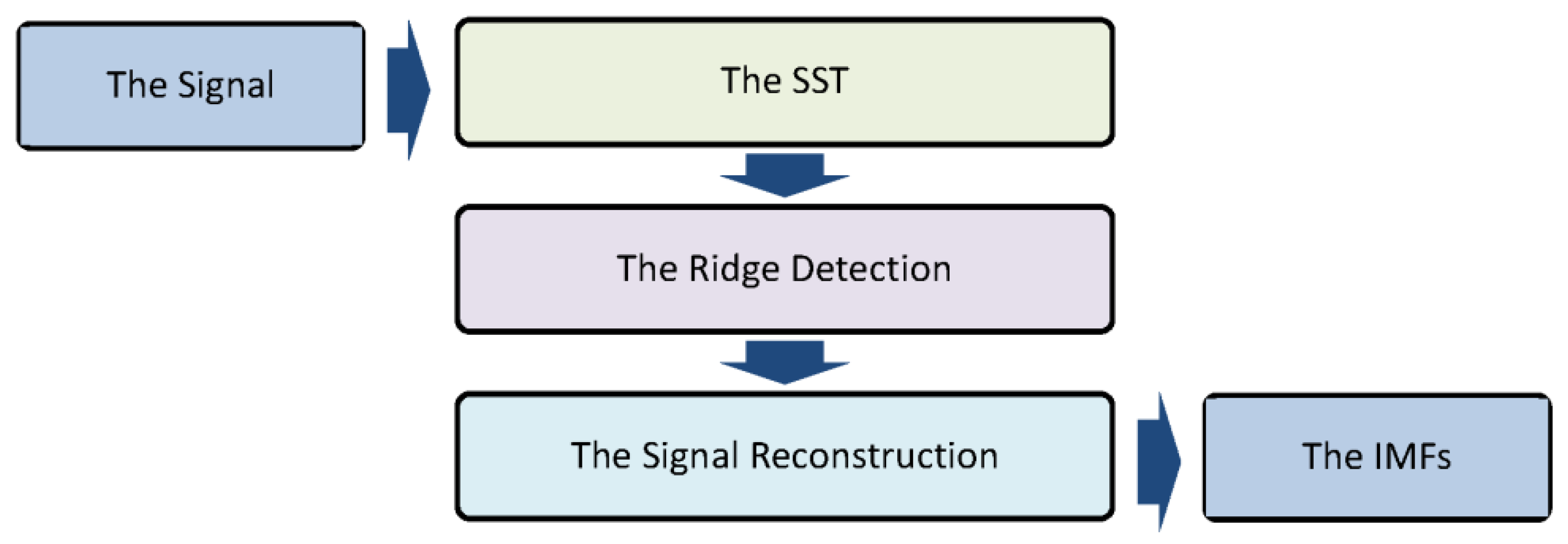
where is the reconstructed IMFs. The decomposition process of the SST is illustrated in Figure 1. This figure illustrates the decomposition process of the SST. The input signal is first transformed into the time–frequency domain using the Continuous Wavelet Transform (CWT). The resulting time–frequency representation is then reassigned to produce a more focused representation, from which the Intrinsic Mode Functions (IMFs) are extracted. This process allows for the separation of signal components with varying frequencies and amplitudes [11].
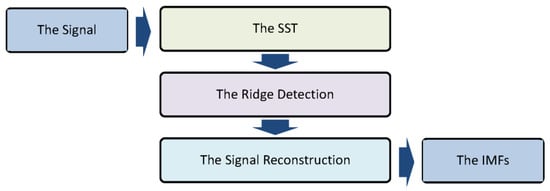
Figure 1.
The decomposition process of the SST.
3. The ESST
3.1. The Method
From what was said in the last section, it seems that there are some problems with using the SST:
- The need to select the “a priori” basis is one of the most critical limitations of the wavelet transform. The “mother wavelet” is usually chosen by trial and error. Even though the choice of wavelet basis has a significant effect on the results, there is no set way to choose the wavelet basis.
- The performance of the ridge detection method is influenced by several parameters, such as the penalty term, the number of frequency bins separated at any ridge detection iteration, and the number of frequency bins added in any reconstruction iteration. There is no systematic way to select these parameters.
- Once the IMFs are reconstructed, the decomposition performance is not checked against any criteria. While the TFRs are qualitatively examined in the literature, there is no quantitative framework for verifying the reconstructed IMFs.
To address these drawbacks, the ESST introduces specific IMF quality criteria to evaluate the fitness of the resulting IMFs.
- Dissimilar IMFs should not contain identical frequency contents at a single time step. In other words, they should be orthogonal. In an ideal case, the scalar product of any two IMFs should vanish. However, orthogonality is not guaranteed due to the computational procedures. The Orthogonality Criterion (OC) may be defined as follows:
where f(t) is the original signal and fk(t) is an IMF.
- The energy content of the signal should be equal to the sum of the energy contents of the IMFs. In an ideal case, the energy should be preserved by the decomposition. Nevertheless, this condition may be neglected by the computational procedures. The Energy Criterion (EC) may be defined as follows:
in which the energy content of the signal f(t) is defined as .
- If the decomposition of the signal and the reconstruction of the IMFs are ideally performed, the mean squared error between the signal and the sum of its IMFs should vanish. However, due to the computational procedures, this condition may be violated. The Mean Squared Error Criterion (MSEC) may be defined as follows:
where n is the number of samples and .
The ESST proposes using the Genetic Algorithm (GA) to find the optimal IMFs of a signal. To this end, the decision parameters of the SST (i.e., the wavelet basis, the penalty term, the number of frequency bins separated at any ridge detection iteration, and the number of frequency bins added in any reconstruction iteration) should be selected in a way that the IMF quality criteria (i.e., the OC, EC, and MSEC) are minimized.
The GA is a multi-agent, direct, and stochastic metaheuristic search method that may find a global optimum within the search space. The GA encodes candidate solutions as strings, known as individuals or chromosomes. It begins with a population of randomly selected individuals. In any iteration of the search process called generation, all the individuals are evaluated against the objective function. The individuals with the highest fitness are more likely to be selected as the next generation’s parents. The selected individuals are influenced by genetic operators such as cross-over and mutation. The individuals stochastically replace the offspring with the lowest fitness. According to the natural selection law, any generation may have better features than the previous one; therefore, evolution results in better individuals. Once the optimization process is stopped, the best individual should be decoded to find the best solution.
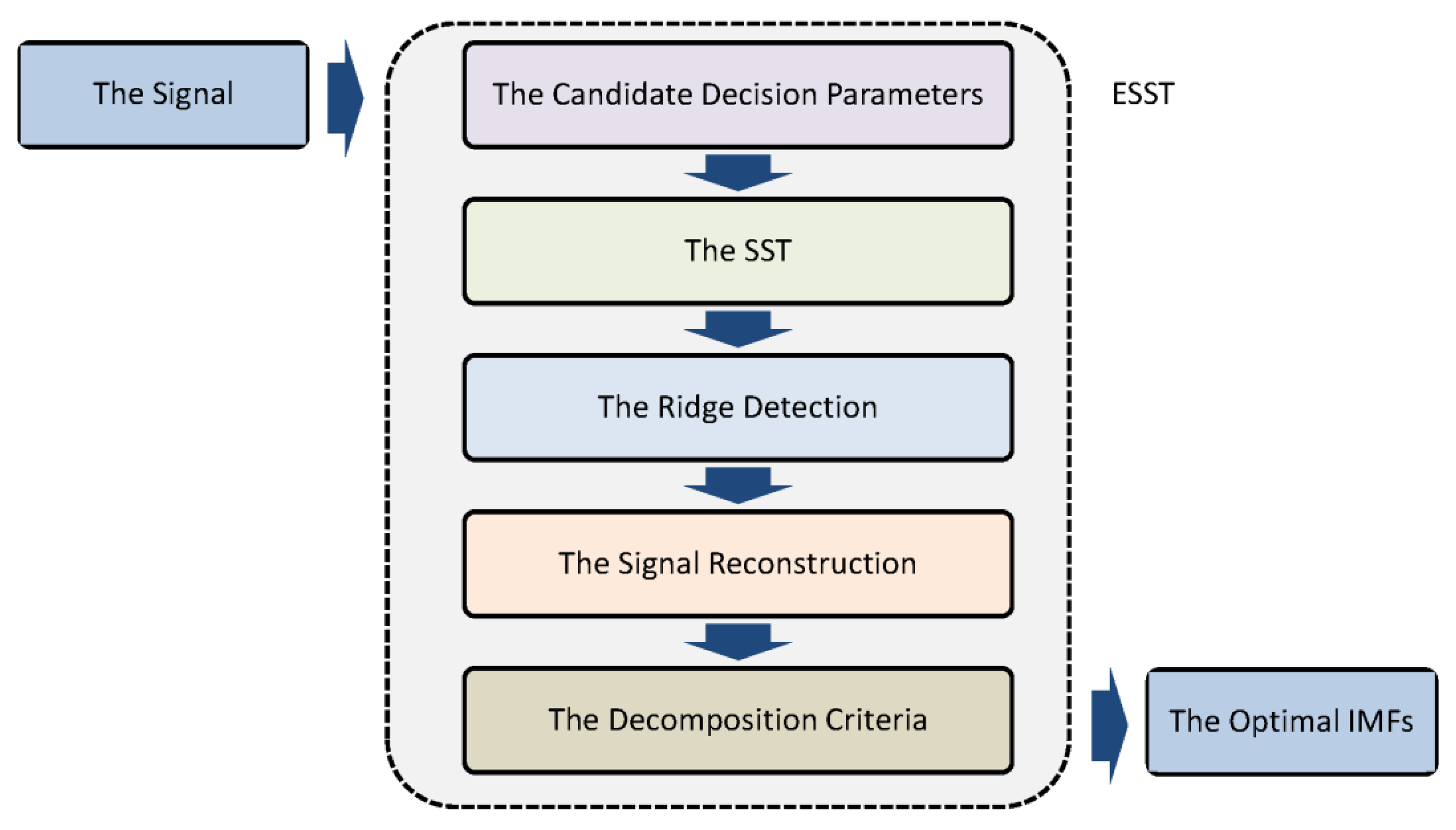
The flowchart of the ESST is illustrated in Figure 2, which outlines the steps of the ESST algorithm. The process begins with the initialization of the Genetic Algorithm (GA) parameters, followed by the selection of the optimal wavelet basis and ridge detection parameters. The signal is then decomposed into IMFs, and the quality of the decomposition is evaluated using the Orthogonality Criterion (OC), Energy Criterion (EC), and Mean Squared Error Criterion (MSEC). The algorithm iteratively refines the parameters until the optimal IMFs are obtained.

Figure 2.
The flowchart of the ESST.
The parameters for the Genetic Algorithm (GA) were carefully selected to balance computational efficiency and optimization accuracy. For instance, the population size of 20 was chosen to ensure a diverse search space without excessive computational demands. The crossover fraction of 0.8 was set to maintain sufficient exploration of the solution space while preserving high-quality individuals. Similarly, the penalty term was initialized at 10 to appropriately penalize high-energy ridge deviations and guide the optimization process effectively. These parameters were fine-tuned based on iterative testing with benchmark signals to achieve robust and reliable results.
The GA optimization utilized for IMF extraction within the ESST is a heuristic-based approach. While this method does not provide systematic guarantees for robustness across all conceivable flight conditions, it offers flexibility in adjusting to varying signal complexities due to its adaptive nature. The effectiveness of the GA-based IMF extraction has been qualitatively validated through diverse signal scenarios in the current study, demonstrating its capability to handle nonlinear and non-stationary dynamics inherent in high angle of attack flights. Future research could investigate its performance under broader experimental conditions to ensure comprehensive robustness.
It should be mentioned that recent advancements in SST, primarily enhance time-frequency resolution or multicomponent separation for specific applications. In contrast, the ESST proposed here addresses the SST’s inherent limitations in parameter dependency and lack of decomposition validation. By combining GA-based optimization with quantitative IMF criteria (OC, EC, MSEC), ESST achieves reliable extraction of dynamic modes, even in highly nonlinear regimes.
3.2. Verification
To verify the ESST, a benchmark signal introduced by [25] is numerically studied. To this end, a comparison is made between the IMFs reconstructed by the SST and ESST. Suppose the following non-stationary signal has two components, namely, a chirp signal of and a damped sinusoidal signal of
where:
and , with a sampling rate of 1024 Hz.
For the SST implementation, we select the analytic Morlet wavelet as the “a priori” basis due to its optimal time–frequency resolution and proven effectiveness in aircraft dynamics analysis [15,22]. The signal is not symmetrically extended to prevent artificial mode creation at boundaries while preserving authentic flight characteristics. We employ a penalty term of 2 multiplied by the squared separation between frequency bins, determined empirically to effectively penalize unrealistic frequency jumps without over-constraining natural mode variations. During ridge detection, four frequency bins are separated at each iteration to balance computational efficiency with accurate mode separation, while 16 frequency bins are added during reconstruction at both sides of the ridge to ensure sufficient bandwidth for complete mode characterization without sacrificing resolution. These parameter selections were systematically optimized through sensitivity analyses on benchmark flight data. For the ESST, the GA with the parameters specified in Table 1 is used.

Table 1.
The GA parameters for the ESST.
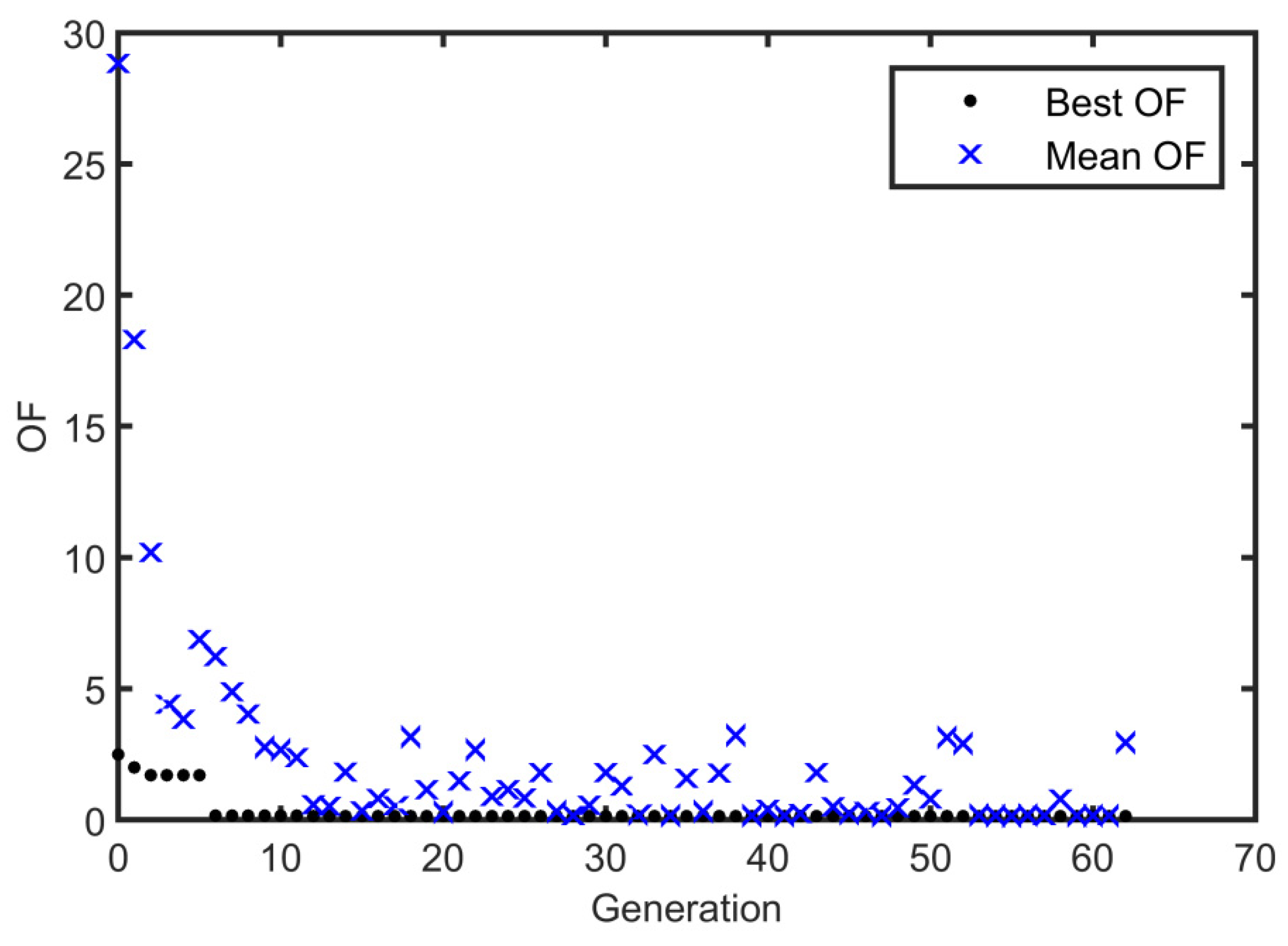
The Objective Function (OF) defines a weighted sum of the IMF quality criteria as follows:
It should be noted that the values of the OC are an order of magnitude less than those of the EC and MSEC; therefore, the OC is multiplied by 10 in the OF. The best and mean values of the OF are plotted against the number of generations in Figure 3. It can be seen that the OF has converged to its best value after 62 iterations.
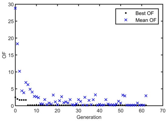
Figure 3.
The OF against the number of generations.
The decision parameters and the IMF quality criteria for the SST and ESST are compared in Table 2. As can be seen from the table, the OFs for the SST and ESST are 46.8992 and 0.1522, respectively. Also, the IMF quality criteria for the ESST are significantly smaller than those for the SST. From an IMF quality point of view, this means that the ESST does better than the SST.
Table 2.
A comparison between the decision parameters and IMF quality criteria for the SST and ESST.
Since the ESST utilizes the GA metaheuristic, it is not possible to provide a formal complexity analysis; however, a comparison is made between the computational time of the SST and ESST. To this end, an 11th Gen Intel(R) Core(TM) i7-11800H @2.30 GHz processor with 16.0 GB of installed RAM is used on a Windows PC. Since the needed time is different for dissimilar runs, an average of over 10 runs is obtained. The results are presented in Table 2. As can be seen, the ESST requires more computational time due to the use of the GA metaheuristic.
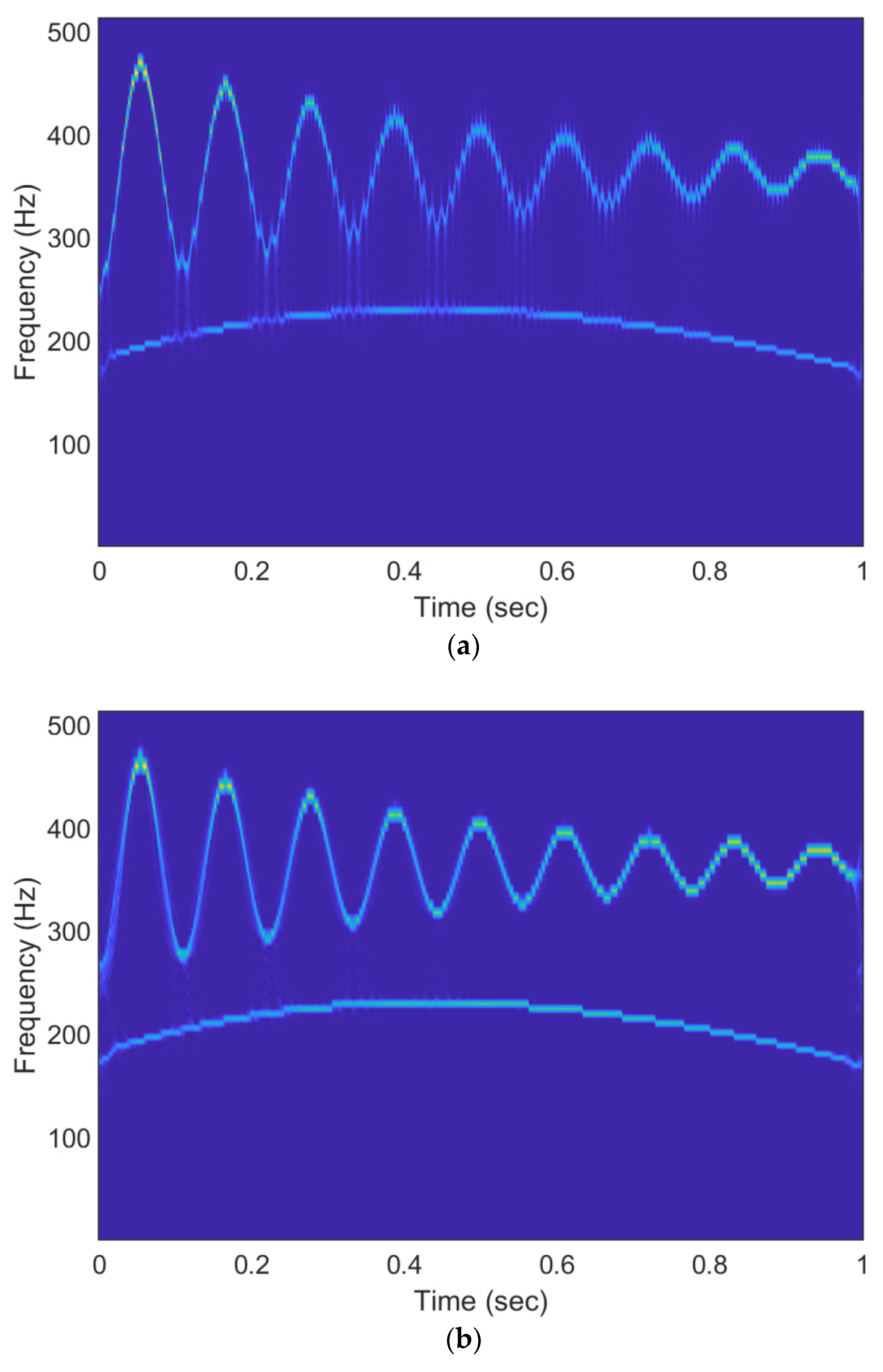
Finally, the TFRs obtained by the SST and ESST are shown in Figure 4. The existence of two AMFM modes can be seen in both cases. According to Equations (13) and (14), the chirp signal of and the damped sinusoidal signal of can be easily recognized in both TFRs. Nevertheless, it can be observed that the TFR provided by the ESST is more “readable”. The SST disperses energy, while the ESST provides a sharper, more focused representation.
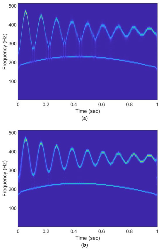
Figure 4.
Superior ability of ESST in accurately capturing TFRs characteristics: (a) SST and (b) ESST.
While the benchmark signal (from Ref. [25]) uses separated frequencies to facilitate comparison with classical SST, real flight data (Section 5) inherently contain overlapping modes. While fixed-parameter methods like [26] effectively address frequency overlaps in their target applications, ESST’s GA-based optimization provides additional flexibility by automatically adapting to crossing frequencies through orthogonality error (OC) minimization, making it particularly suitable for complex flight dynamics scenarios.
4. Instantaneous Characteristics of the Flight Modes
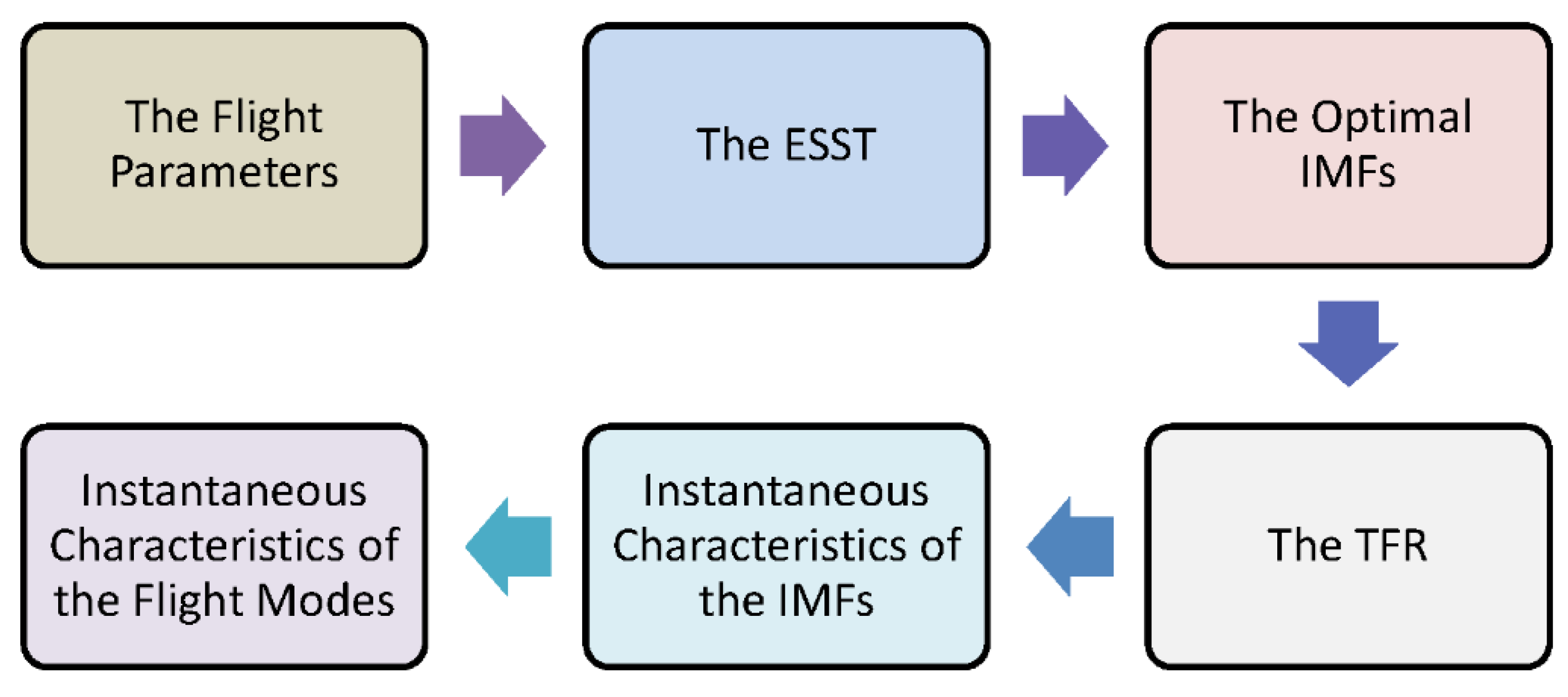
This section outlines a method to determine the instantaneous characteristics of ESST-derived flight modes. Initially, it analyzes longitudinal and lateral/directional flight parameters. Then, the TFRs are provided, and the ridges with the highest energy are isolated. Next, the optimal IMFs corresponding to the detected ridges are reconstructed. Afterward, the instantaneous characteristics of the IMFs (i.e., frequency, amplitude, and phase) are obtained. Finally, the instantaneous characteristics of the flight modes (i.e., the undamped natural frequency and damping ratio) are calculated using the IMF characteristics.
Suppose that a flight parameter is composed of K AMFM flight modes. According to Equation (1), the instantaneous amplitude and phase of the kth IMF can be represented as follows:
In which and are damped and un-damped natural frequencies, and is the damping ratio of the kth IMF. Thus, it is clear that:
Since , the instantaneous characteristics of the kth flight modes (i.e., the un-damped natural frequency and damping ratio) can be found as follows:
The flowchart for obtaining the instantaneous characteristics of the flight modes is summarized in Figure 5. The process involves extracting the ridges from the time–frequency representation, reconstructing the corresponding IMFs, and calculating the instantaneous frequency, amplitude, and phase. These characteristics are then used to determine the undamped natural frequency and damping ratio of each flight mode.
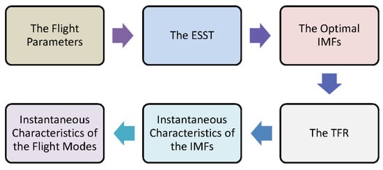
Figure 5.
The flowchart for obtaining the instantaneous characteristics of the flight modes.
5. Results and Discussion
5.1. Flight Data
In this study, flight data of a large-scale Remotely Piloted Vehicle (RPV) provided by Ref. [26] is studied. The primary aim of Ref. [27] was to investigate the aerodynamic characteristics of the RPV at high angles of attack flights and post-stall maneuvers. Since the aerodynamic characteristics had the highest priority, the RPV was unpowered, and the open-loop control system was employed in many flight tests. Furthermore, the control surfaces were aerodynamically activated. Also, a control system was used to apply the control commands independently. The RPV was dropped from a large airplane and recovered in midair by a helicopter. The geometric parameters, weight and balance, and moments of inertia of the RPV are summarized in Table 3.
Table 3.
The geometry parameters of the RPV [27].
There are several reasons for studying the flight data presented by Ref. [27] from the aircraft system identification point of view: Firstly, the studied RPV was unpowered; therefore, it is possible to examine the high angle of attack aerodynamics affected by the conventional aerodynamic surfaces without considering the effects of the thrust forces and moments as well as the thrust vectoring. Secondly, the RPV had an un-augmented flight control system in some flight tests; therefore, it is possible to check the open-loop characteristics of the RPV during the high angle of attack maneuvers in the absence of the flight control systems. Finally, various longitudinal and lateral/directional flight parameters are reported under different conditions. The flight tests were performed at extremely high angles of attack to investigate the stability and controllability of the aircraft at post-stall maneuvers. During the flight tests, the angle of attack up to 80 degrees was reached. Several flight tests were performed under different flight conditions. Flight data was obtained using a variety of sensors and transmitted to the flight control station, where the data was gathered and the control commands were applied. The actual flight data were sampled at a rate of 40 samples per second; however, they are digitized in this study at a rate of 20 samples per second.
5.2. The Application of the ESST
In comparison to traditional methods such as the SST, HHT, and wavelet methods, the ESST demonstrates a superior capability in detecting non-traditional flight modes in high angle of attack maneuvers. Through a series of numerical simulations and flight test data, it is shown that ESST outperforms these existing methods by providing clearer decomposition and capturing transient flight dynamics more effectively.
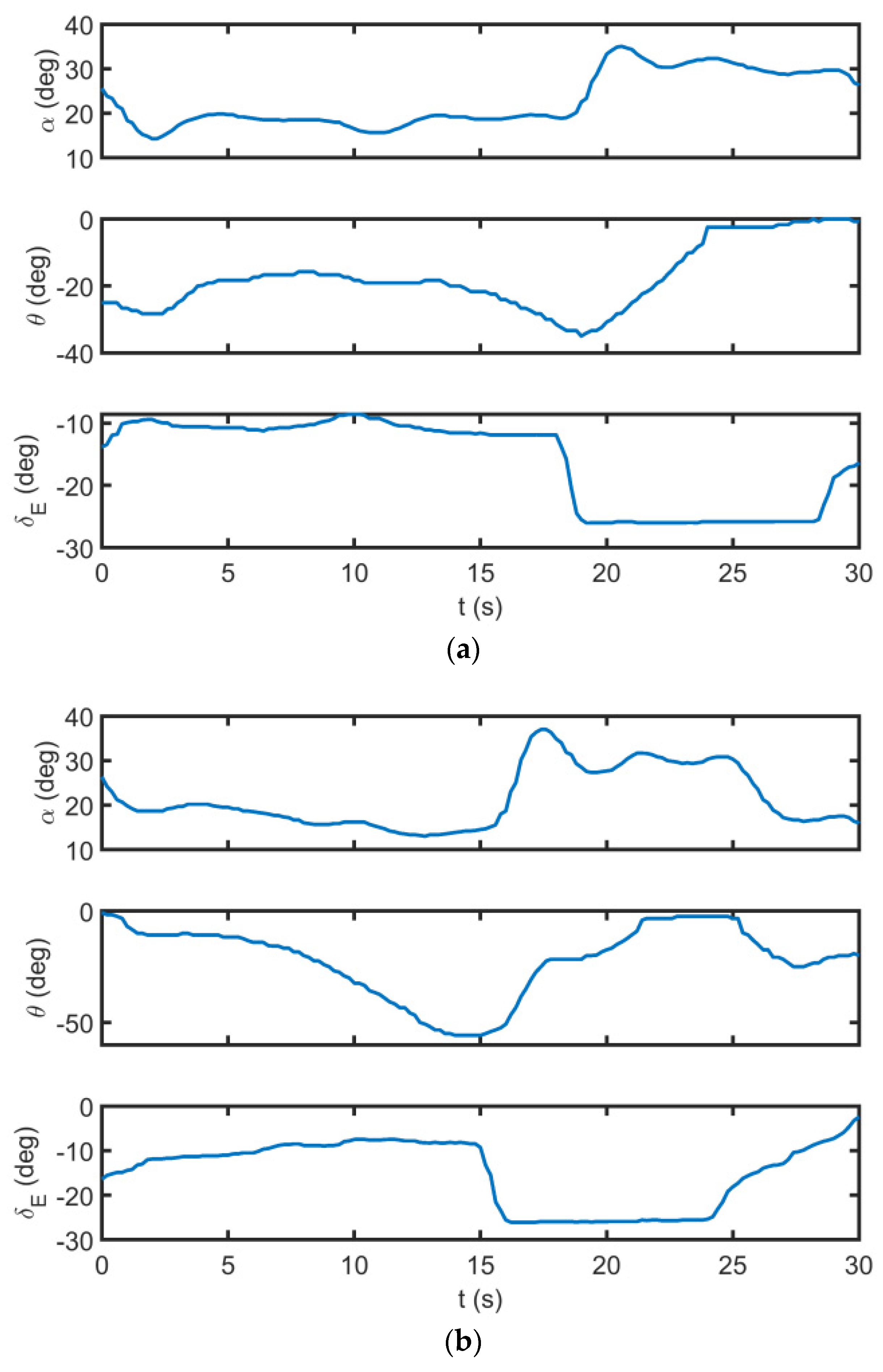
This paper uses two flight datasets to validate the extracted flight modes. The time histories of the longitudinal flight parameters for datasets A and B are presented in Figure 6. As can be seen, the flight tests are performed by similar elevator doublet commands; nevertheless, the initial flight conditions are different.
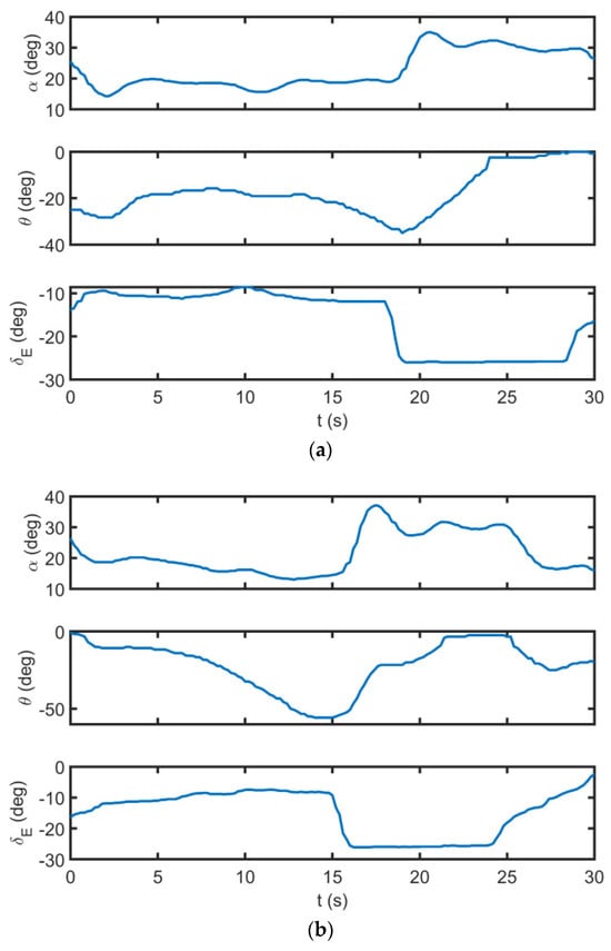
Figure 6.
The time history of longitudinal flight parameters for (a) dataset A and (b) dataset B.
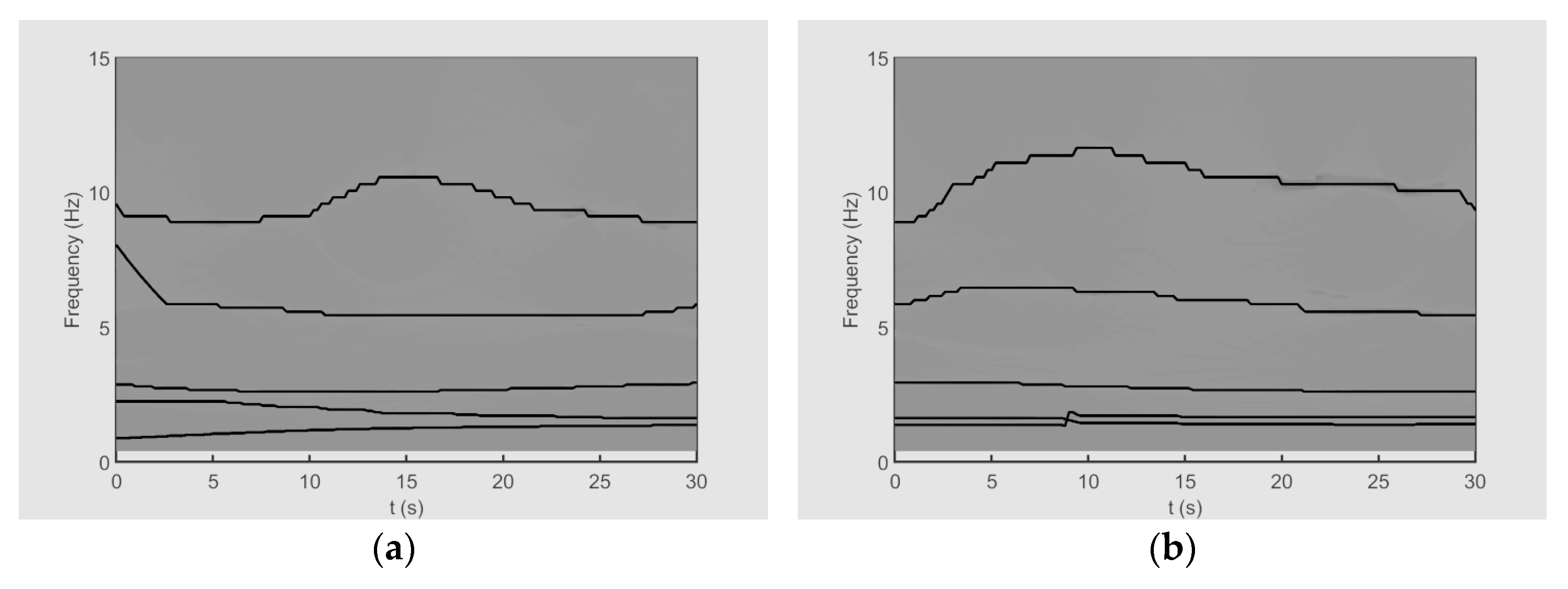
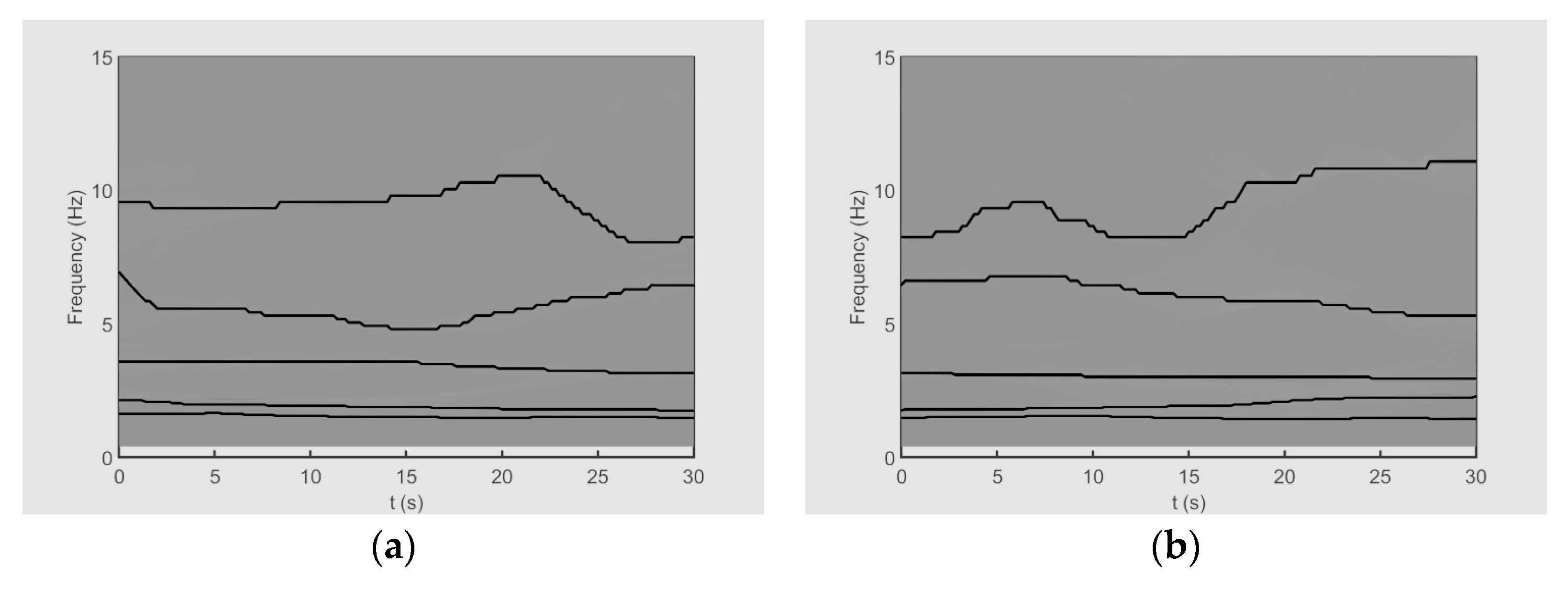
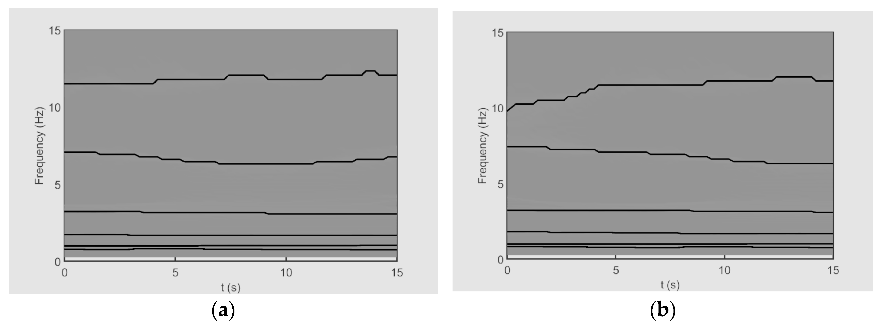
The ESST is applied to both of the time histories, with its performance compared against conventional CWT analysis. The TFRs of the angle of attack (Figure 7) and pitch angle (Figure 8) reveal five distinct high-energy ridges for both datasets, marked by black lines. While CWT analysis shows significant spectral smearing (particularly below 2 Hz), ESST maintains sharp frequency localization, enabling clear separation of adjacent modes. This is especially evident for the non-traditional modes (IMF3-5) that appear merged in CWT but are distinctly resolved by ESST’s adaptive optimization and reassignment mechanism. The extracted ridges demonstrate similar frequency content across both figures, verifying identical flight modes under different conditions. Notably, during rapid maneuvers (t = 12–18 s), ESST precisely tracks instantaneous frequency variations that CWT fails to capture, confirming its superior resolution for analyzing complex flight dynamics.
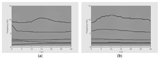
Figure 7.
The TFRs of the angle of attack for (a) dataset A and (b) dataset B.
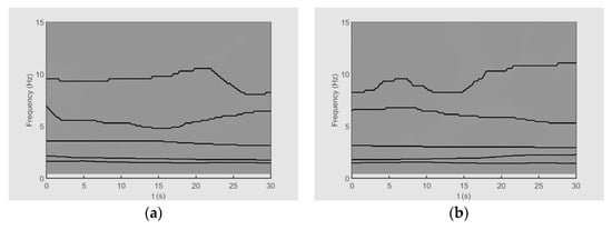
Figure 8.
The TFRs of the pitch angle for (a) dataset A and (b) dataset B.
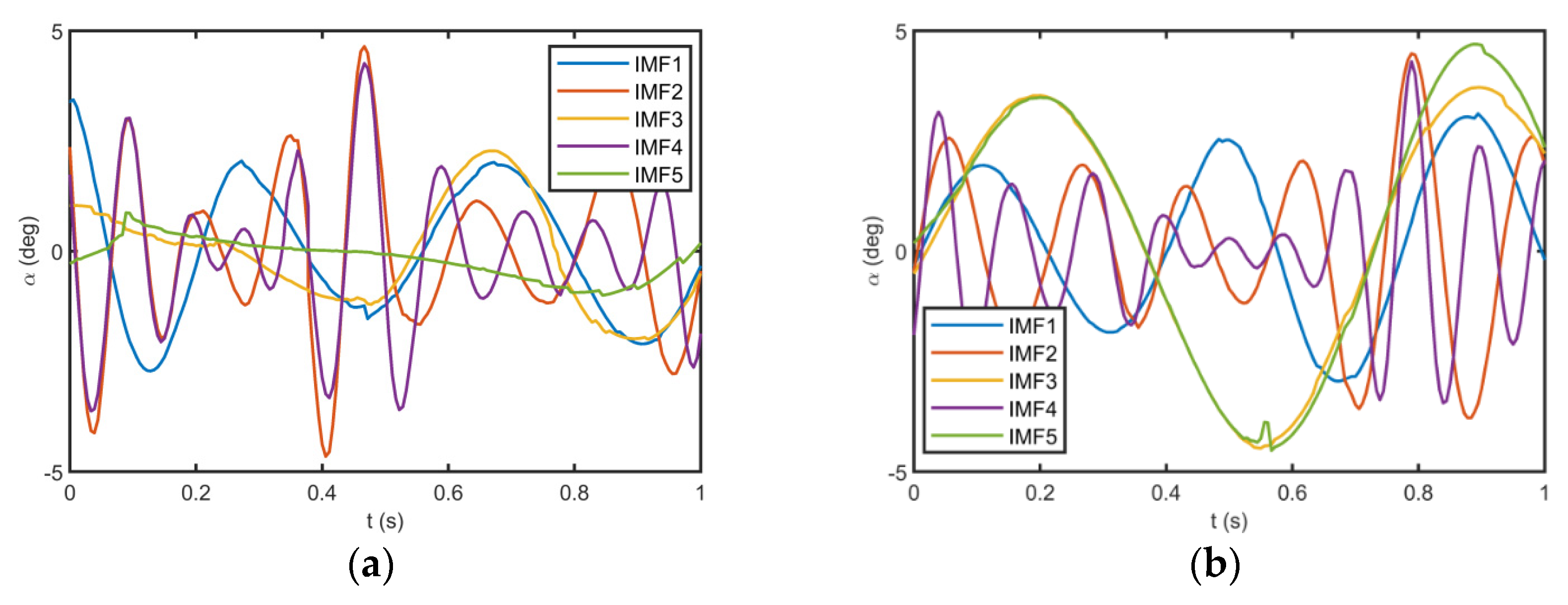
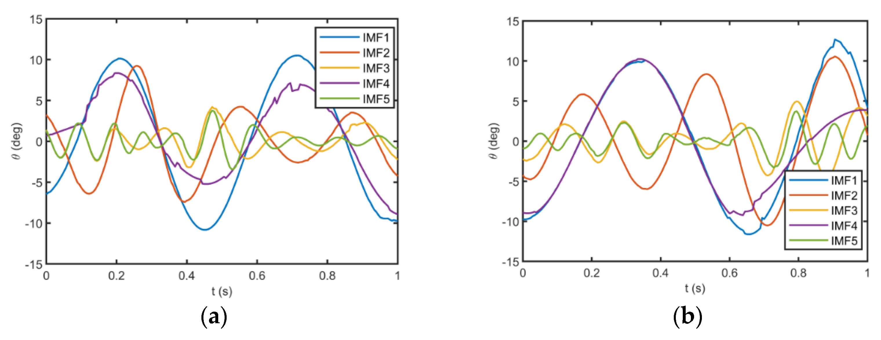
The ESST reconstructs the optimal IMFs that correspond to the detected high-energy ridges. The optimal IMFs of the angle of attack and the pitch angle in a one-second interval for both datasets are shown in Figure 9 and Figure 10, respectively. These plots indicate that the flight parameters are decomposed into five non-stationary IMFs. The non-smooth behavior observed in IMF 4 of Figure 10a is attributed to the complex vortex dynamics characteristic of post-stall flight conditions. These irregularities (particularly noticeable at t = 3.2 s and 4.7 s) correspond to: (1) intermittent vortex shedding events at high angles of attack, and (2) rapid control surface adjustments during aggressive maneuvers. The ESST algorithm preserves these physically significant transients by adaptively optimizing its parameters to capture nonlinear interactions without artificial smoothing, unlike conventional decomposition methods that might suppress such features. This fidelity to actual flight dynamics is crucial for accurate identification of non-traditional flight modes.
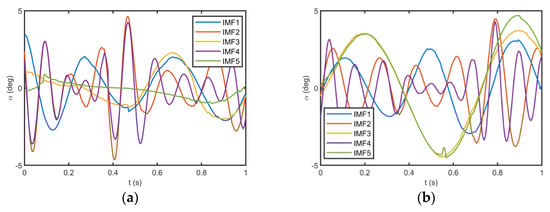
Figure 9.
The optimal IMFs of the angle of attack for (a) dataset A and (b) dataset B.
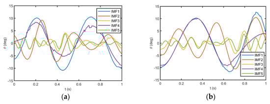
Figure 10.
The optimal IMFs of the pitch angle for (a) dataset A and (b) dataset B.
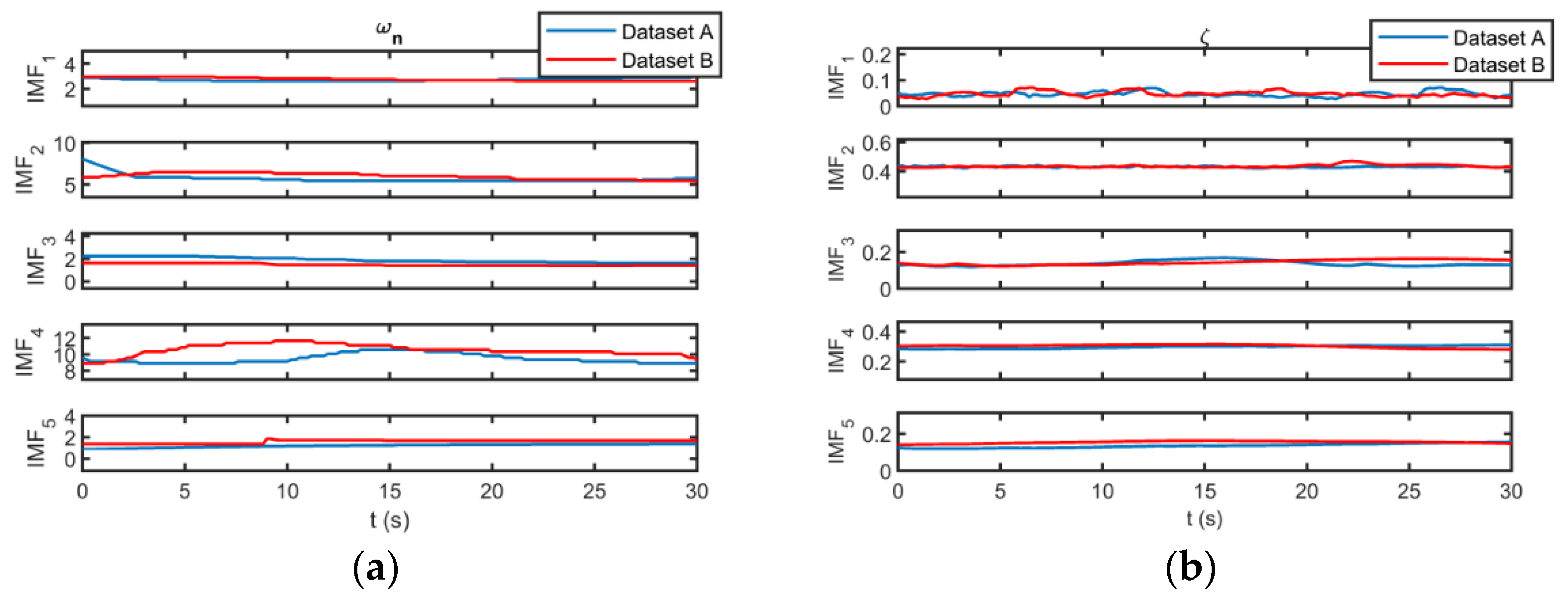
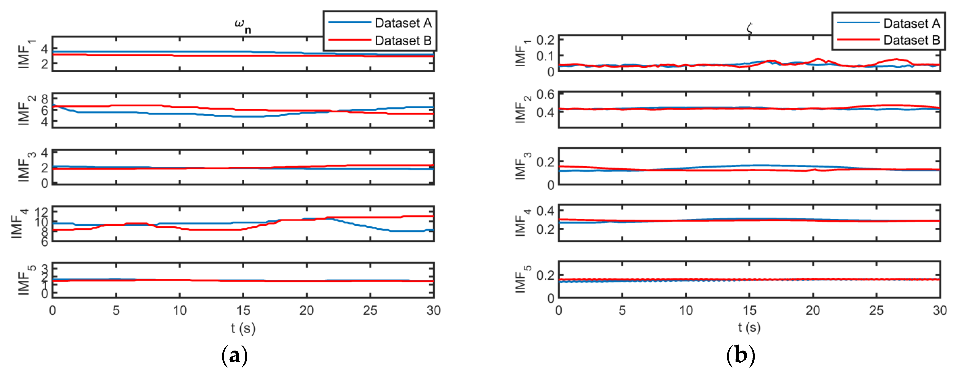
Once the optimal longitudinal IMFs are extracted, the instantaneous characteristics of flight modes can be calculated using the method described in Section 4. The instantaneous undamped natural frequency and damping ratio of the angle of attack and pitch angle for both datasets are illustrated in Figure 11 and Figure 12. As can be seen, the corresponding IMFs for datasets A and B have similar instantaneous undamped natural frequencies and damping ratios. In other words, the identified flight modes exist in different datasets. Furthermore, the instantaneous characteristics of the IMFs obtained for the angle of attack are very similar to those of the pitch angle. Hence, the identified flight modes exist in all the longitudinal flight parameters.
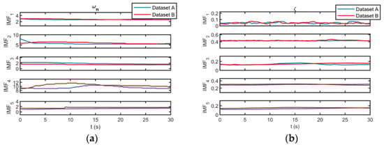
Figure 11.
(a) The instantaneous undamped natural frequency and (b) the instantaneous damping ratio of the angle of attack for both of the datasets.
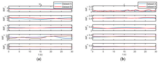
Figure 12.
(a) The instantaneous undamped natural frequency and (b) the instantaneous damping ratio of the pitch angle for both of datasets.
The results indicate some “non-traditional” modes that the classical flight dynamic model cannot predict. These modes are non-stationary; therefore, their characteristics are altered instantaneously. Table 4 and Table 5 show the mean value, range, and standard deviation of the longitudinal flight modes obtained from datasets A and B.
Table 4.
The characteristics of the longitudinal flight modes obtained from datasets A.
Table 5.
The characteristics of the longitudinal flight modes obtained from datasets B.
Comparing the longitudinal flight modes identified by the ESST with the longitudinal “traditional” modes obtained by the classical model is necessary. The “traditional” modes can be found by solving the longitudinal characteristic equation as follows:
The constants A, B, C, D, and E are found using the non-dimensional stability and control derivatives. For more details about the longitudinal transfer functions, one may see Ref. [27]. The UAV’s non-dimensional stability and control derivatives are listed in Table 6 based on the data provided by Ref. [27].
Table 6.
The non-dimensional stability and control derivatives for the UAV.
Using the aforementioned stability and control derivatives, one may obtain the following longitudinal characteristic equation for the UAV:
The traditional longitudinal modes obtained by solving the above equation are presented in Table 7. It can be seen that there are two traditional longitudinal modes, namely, a low-frequency, slowly damped mode called the Phugoid (P) and a high-frequency, highly damped mode called the Short Period (SP).
Table 7.
The characteristics of the P and SP modes of the UAV.
It can be seen that the natural undamped frequency and the damping ratio of the SP mode are very similar to those of the IMF_2. Thus, it can be concluded that the ESST recognizes the SP mode. Nevertheless, after comparison of the P mode characteristics with the IMF ones, it can be seen that the P mode is not discovered. This inconsistency may be because the P mode for this aircraft is unstable with a very low frequency. The time to double the amplitude in the P mode can be calculated by the following equation [28]:
For this aircraft, the time to double the amplitude in the P mode is 2139 s; therefore, it is not surprising that the ESST does not reveal the P mode.
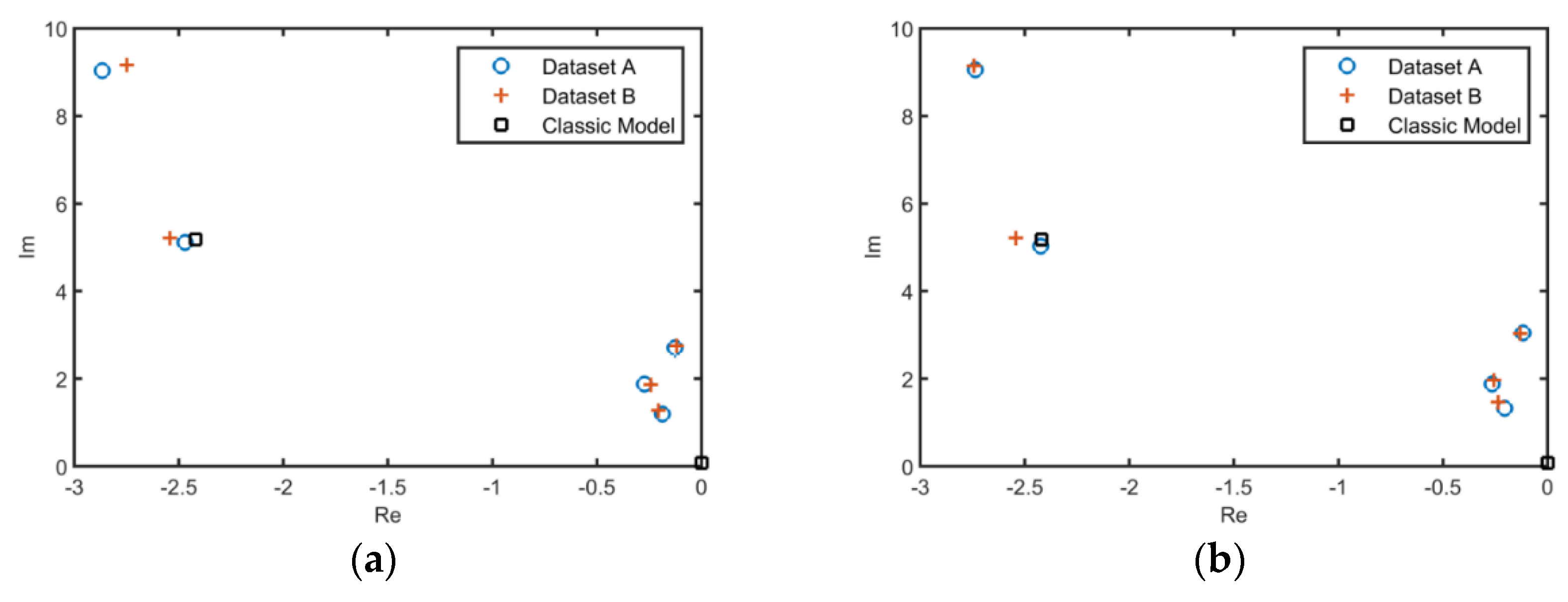
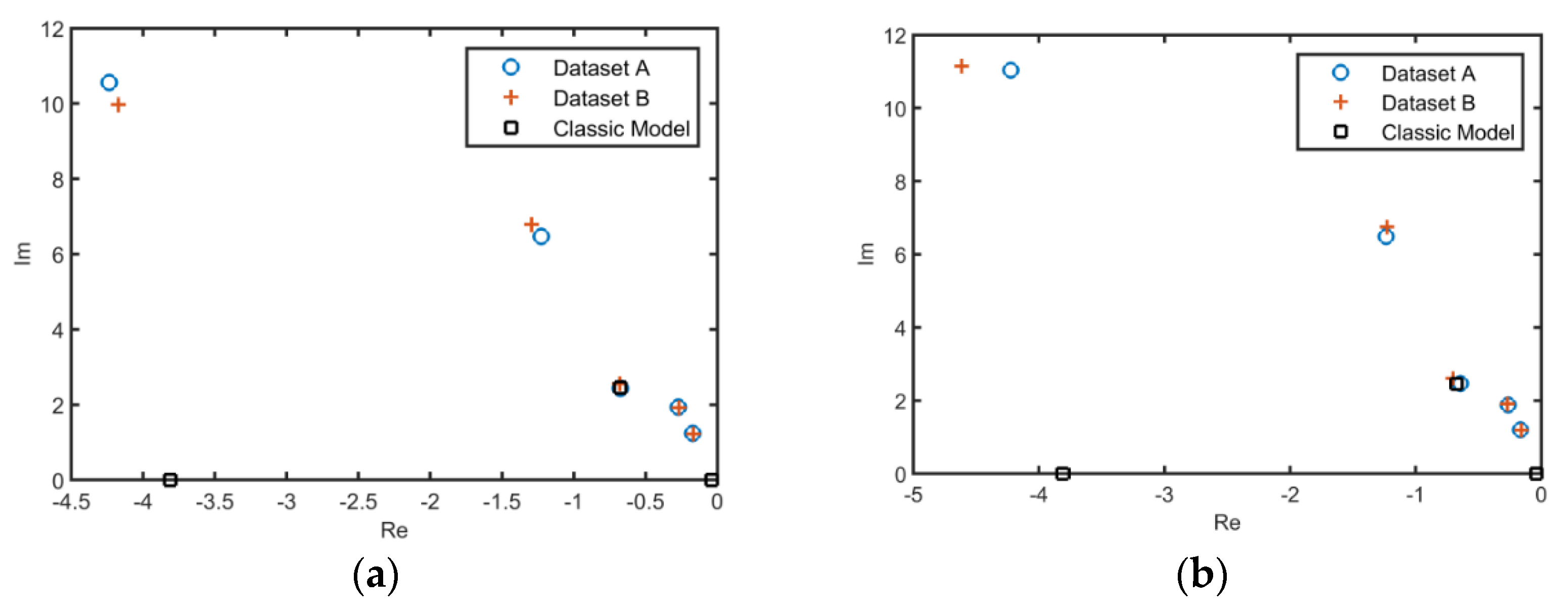
In addition to the SP mode, four “non-traditional” modes have been discovered by the ESST. While the IMF_4 is a high-frequency and moderately damped mode, the IMF_1, IMF_3, and IMF_5 are low-frequency and slowly damped ones. The details of the longitudinal modes obtained by the ESST are reported in Table 4 and Table 5. For more clarity, the longitudinal flight modes obtained by the ESST are illustrated in Figure 13 using the corresponding mean values of the undamped natural frequency and damping ratio. Furthermore, the “traditional” modes obtained by the classical model are illustrated in Figure 13.
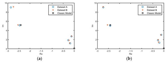
Figure 13.
The longitudinal flight modes obtained from (a) the angle of attack and (b) the pitch angle.
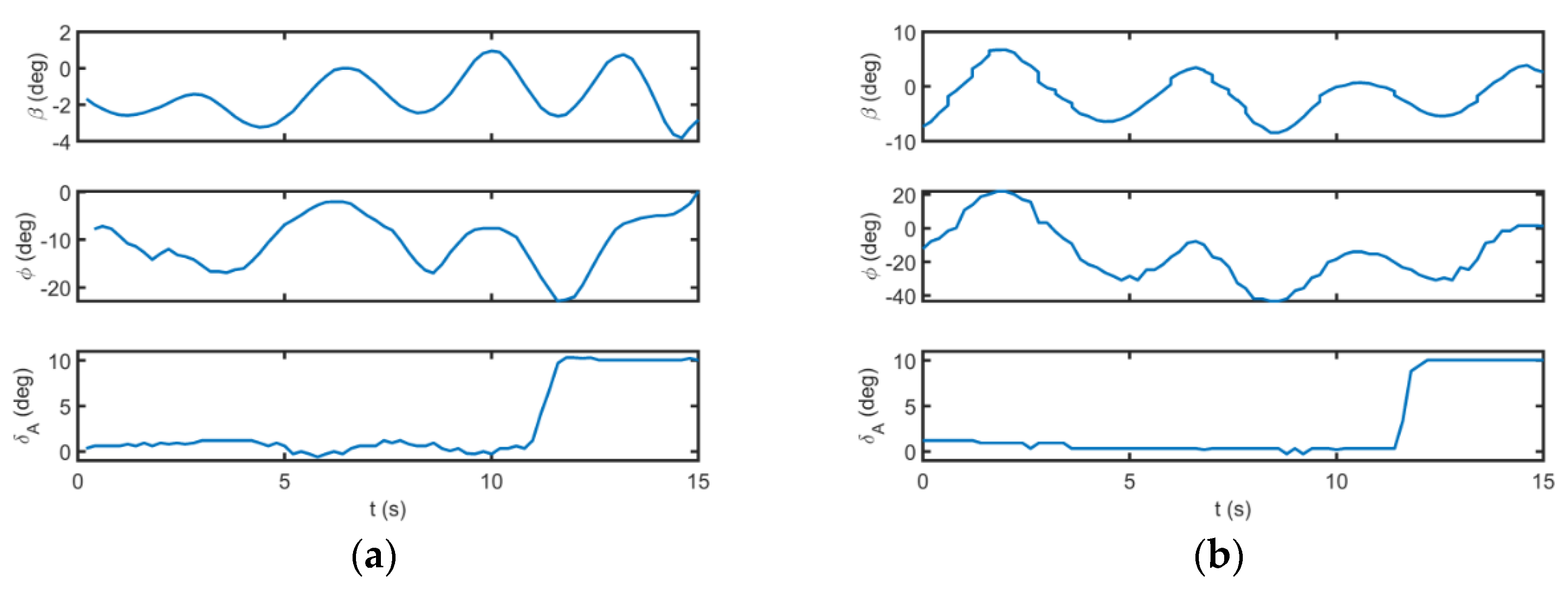
The ESST is also applied to the lateral flight parameters. The time histories of lateral flight parameters are illustrated in Figure 14 for datasets A and B. As can be seen, the flight tests are performed by similar aileron step commands; nevertheless, the initial flight conditions of datasets A and B are different.
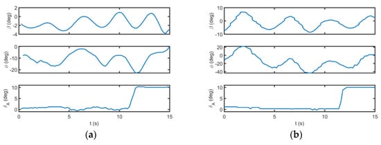
Figure 14.
The time history of lateral flight parameters for (a) dataset A and (b) dataset B.
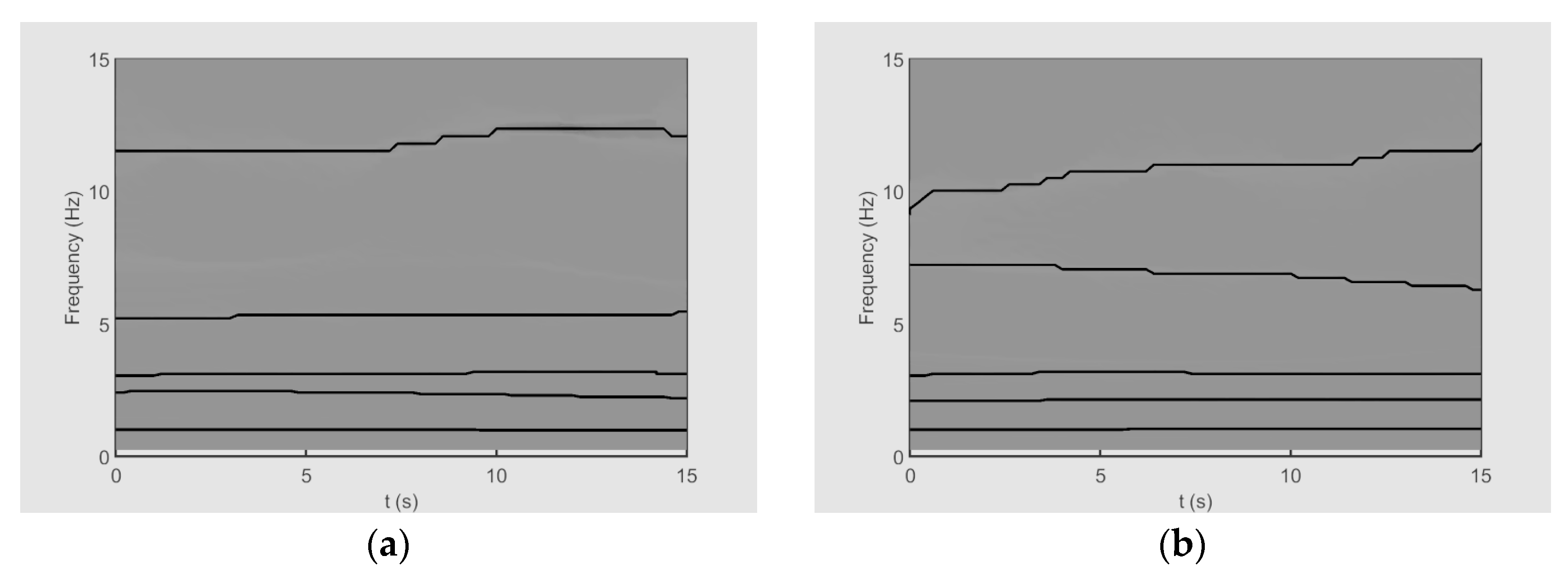
The TFRs of the sideslip angle for datasets A and B are illustrated in Figure 15. Also, the TFRs of the roll angle for datasets A and B are shown in Figure 16. In these figures, the ridges corresponding to the optimal IMFs obtained by the ESST are plotted by black lines. It can be seen that the sideslip angle and the roll angle have five high-energy ridges for both datasets. Based on the results, the extracted IMFs have similar frequency content. This observation verifies the existence of identical “non-traditional” flight modes with non-stationary characteristics at different flight conditions.
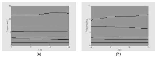
Figure 15.
The TFRs of the sideslip angle for (a) dataset A and (b) dataset B.
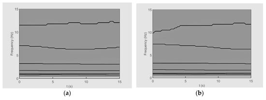
Figure 16.
The TFRs of the roll angle for (a) dataset A and (b) dataset B.
The optimal lateral IMFs and their instantaneous characteristics are not mentioned to avoid lengthening the paper. Table 8 and Table 9 summarize the mean value, range, and standard deviation of lateral flight modes from datasets A and B.
Table 8.
The characteristics of the lateral flight modes obtained from datasets A.
Table 9.
The characteristics of the lateral flight modes obtained from dataset B.
To be compared with the flight modes identified by the ESST, the lateral “traditional” modes obtained by the classical model are also determined. The lateral characteristic equation can be attained as mentioned in Equation (19), where the constants A, B, C, D, and E are obtained by the non-dimensional stability and control derivatives. The utilized non-dimensional stability and control derivatives for the current aircraft are listed in Table 6. According to Table 6, the following lateral characteristic equation is calculated:
It can be seen that the natural un-damped frequency and the damping ratio of the DR mode are very similar to those of the IMF4. Thus, it can be concluded that the ESST recognizes the DR mode. Nevertheless, the ESST cannot capture the first-order convergent modes of S and R.
In addition to the DR mode, four “non-traditional” modes have been discovered by the ESST. The existence of these flight modes is confirmed through both different datasets and flight parameters. It can be seen that the IMF1 is a high-frequency and moderately damped mode, the IMF3 is a moderate-frequency and slowly damped one, and IMF2, IMF5 are low-frequency and slowly damped ones. The lateral flight modes obtained by the ESST are illustrated in Figure 17 using the corresponding mean values of the un-damped natural frequency and damping ratio. Also, Figure 17 shows the “traditional” lateral modes obtained by the classical model.
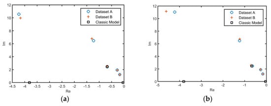
Figure 17.
The lateral flight modes obtained from (a) the sideslip angle and (b) the roll angle.
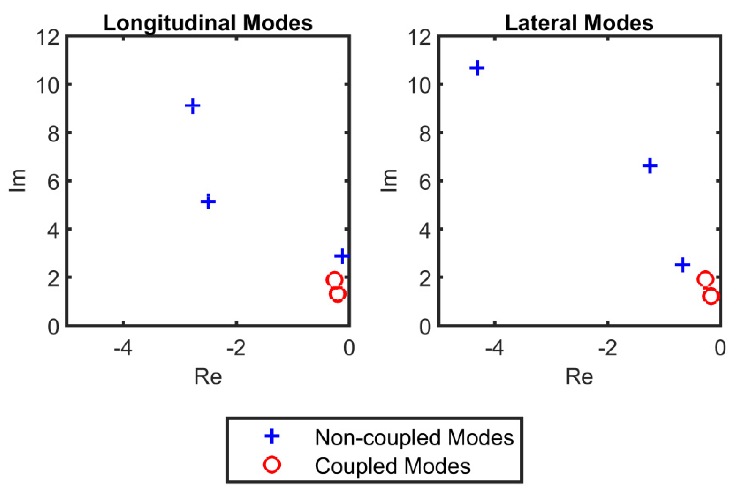
Finally, the longitudinal and lateral modes reconstructed by the ESST are compared in Figure 18 by averaging their instantaneous characteristics. It can be seen that there are two longitudinal and two lateral modes with almost identical characteristics. So, we can say that these are coupled modes that happen simultaneously in both the longitudinal and lateral dynamics.
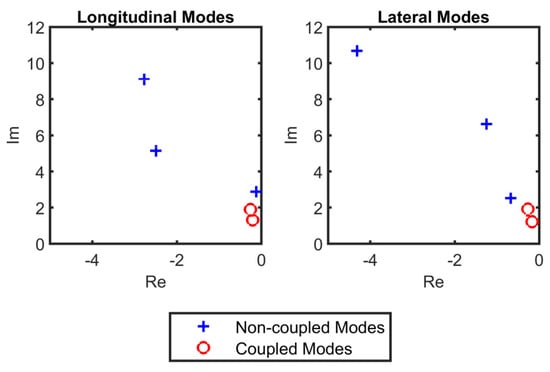
Figure 18.
The comparison between the longitudinal and lateral modes obtained by the ESST.
These findings underscore the capability of the ESST to identify both classical and ‘non-traditional’ flight modes with high precision. By providing sharper Time–Frequency Representations and isolating coupled modes, the ESST advances the understanding of complex flight dynamics in high angle of attack regimes. These insights have significant implications for high-fidelity stability analysis, controller design, and simulation in aerospace engineering. However, it is important to consider its limitations. Certain scenarios, such as the presence of high levels of noise or highly complex flight modes with multiple overlapping non-stationary signals, may challenge the performance of ESST. Additionally, the computational demands of this method may render it less suitable for real-time applications with constrained resources. Addressing these limitations paves the way for future investigations aimed at enhancing its robustness and efficiency under diverse operational conditions.
6. Conclusions
Flight modes should be carefully studied for high-fidelity stability analysis, controller design, and simulation in high angle of attack maneuvers. Recent researches show that “non-traditional” flying modes may occur in high angle of attack flights. Due to the mixed nature of the flight modes, signal decomposition techniques are required to extract them; this paper introduces the ESST approach for this purpose. The ESST decomposes an AMFM signal into its contributing optimal IMFs. The ESST uses the GA to determine the “a priori” basis of the wavelet, the penalty term, the number of frequency bins separated at each ridge detection iteration, and the number of frequency bins added in every reconstruction iteration to optimize the OC, EC, and MSEC of the IMFs. Numerical studies show that the ESST outperforms the SST in terms of IMF quality and TFR resolution.
This paper introduces a method for applying the ESST to actual flight data in order to derive flight modes from the high angle of attack and rapid maneuvering flights. This method is implemented using flight data of a large-scale RPV in post-stall maneuvers. For the verification, two longitudinal and two lateral flight tests were investigated. Based on the results, the longitudinal flight characteristics (i.e., the angle of attack and the pitch angle) are decomposed into five oscillatory components: the SP mode, two high-frequency and moderately damped components, and three low-frequency and slowly damped components. In addition, the lateral flight characteristics (i.e., the sideslip angle and the roll angle) consist of five oscillatory components: the DR mode, a high-frequency and moderately damped component, a moderate-frequency and slowly damped component, and two low-frequency and slowly damped components. Comparisons reveal the simultaneous existence of two coupled modes in both longitudinal and lateral dynamics. Further research should be undertaken to employ the extracted longitudinal, lateral, and coupled flight modes in the flight simulation and controller design at high angles of attack. The main contributions of this study can be summarized as follows:
- -
- Introduction of ESST: The ESST was proposed to overcome the limitations of the traditional SST by incorporating a GA to optimize the decomposition process.
- -
- Identification of Non-Traditional Flight Modes: Using ESST, we successfully identified both traditional and non-traditional flight modes in high angle of attack maneuvers, which were previously undetectable using classical methods.
- -
- Validation with Real Flight Data: The effectiveness of ESST was validated using real flight data from a large-scale RPV, demonstrating its applicability in practical scenarios.
The ESST has significant implications for flight control design, particularly in high angle of attack and rapid maneuver scenarios. By accurately decomposing complex flight signals and identifying “non-traditional” flight modes, the ESST provides critical insights into the dynamic behavior of an aircraft under extreme conditions. This enables the development of more precise and adaptive control strategies, ensuring stability and performance even in challenging flight regimes. Furthermore, the detailed characterization of flight modes using ESST can inform the optimization of control laws and improve the robustness of flight controllers, paving the way for advancements in both manned and unmanned aerial vehicle designs.
Author Contributions
Conceptualization, S.A.B. and H.M.; methodology, S.A.B.; software, S.A.B.; validation, S.A.B., H.M. and M.H.A.; formal analysis, M.H.A.; investigation, H.M.; resources, S.A.B.; data curation, S.A.B.; writing—original draft preparation, M.H.A.; writing—review and editing, H.M.; visualization, H.M.; supervision, S.A.B.; project administration, M.H.A. All authors have read and agreed to the published version of the manuscript.
Funding
This research received no external funding.
Data Availability Statement
The data presented in this study are available on request from the corresponding author, Seyed Amin Bagherzadeh (bagherzadeh@iau.ac.ir).
Conflicts of Interest
The authors declare no conflict of interest.
Abbreviations
| A | amplitude of oscillation |
| a | cylinder diameter |
| CG | center of gravity |
| Cp | pressure coefficient |
| Cx | force coefficient in the x direction |
| Cy | force coefficient in the y direction |
| c | chord |
| dt | time step |
| Fx | X component of the resultant pressure force acting on the vehicle |
| Fy | Y component of the resultant pressure force acting on the vehicle |
| f, g | generic functions |
| h | height |
| i | time index during navigation |
| j | waypoint index |
| K | trailing-edge (TE) nondimensional angular deflection rate |
| Θ | boundary-layer momentum thickness |
| ρ | Density |
| j | imaginary unit |
References
- Andrievsky, B.; Kudryashova, E.V.; Kuznetsov, N.V.; Kuznetsova, O.A. Aircraft wing rock oscillations suppression by simple adaptive control. Aerosp. Sci. Technol. 2020, 105, 106049. [Google Scholar] [CrossRef]
- Mokhtari, S.A.; Sabzehparvar, M. Spin flight mode identification with OEEMD algorithm. Aircr. Eng. Aerosp. Technol. 2019, 91, 582–600. [Google Scholar] [CrossRef]
- Ohmichi, Y.; Ishida, T.; Hashimoto, A. Modal decomposition analysis of three-dimensional transonic buffet phenomenon on a swept wing. AIAA J. 2018, 56, 3938–3950. [Google Scholar] [CrossRef]
- Bagherzadeh, S.A. Flight dynamics modeling of elastic aircraft using signal decomposition methods. Proc. Inst. Mech. Eng. Part G J. Aerosp. Eng. 2019, 233, 4380–4395. [Google Scholar] [CrossRef]
- Bagherzadeh, S.A.; Sabzehparvar, M. Estimation of flight modes with Hilbert-Huang transform. Aircr. Eng. Aerosp. Technol. Int. J. 2015, 87, 402–417. [Google Scholar] [CrossRef]
- Mohammadi, S.J.; Sabzeparvar, M.; KArrari, M. Aircraft stability and control model using wavelet transforms. Proc. Inst. Mech. Eng. Part G J. Aerosp. Eng. 2010, 224, 1107–1118. [Google Scholar] [CrossRef]
- Mokhtari, S.A.; Sabzehparvar, M. Application of Hilbert-Huang transform with improved ensemble empirical mode decomposition in nonlinear flight dynamic mode characteristics estimation. J. Comput. Nonlinear Dyn. 2019, 14, 011006. [Google Scholar] [CrossRef]
- Huang, N.E. Introduction to the Hilbert-Huang transform and its related mathematical problems. In Hilbert-Huang Transform and Its Applications 2014; Springer: Berlin/Heidelberg, Germany, 2014; pp. 1–26. [Google Scholar]
- Meignen, S.; Oberlin, T.; Pham, D.H. Synchrosqueezing transforms: From low-to high-frequency modulations and perspectives. Comptes Rendus Phys. 2019, 20, 449–460. [Google Scholar] [CrossRef]
- Oberlin, T.; Meignen, S.; Perrier, V. The Fourier-based synchrosqueezing transform. In Proceedings of the 2014 IEEE International Conference on Acoustics, Speech and Signal Processing (ICASSP) 2014, Florence, Italy, 4–9 May 2014; pp. 315–319. [Google Scholar]
- Daubechies, I.; Lu, J.; Wu, H.T. Synchrosqueezed wavelet transforms: An empirical mode decomposition-like tool. Appl. Comput. Harmon. Anal. 2011, 30, 243–261. [Google Scholar] [CrossRef]
- Li, Z.; Gao, J.; Li, H.; Zhang, Z.; Liu, N.; Zhu, X. Synchroextracting transform: The theory analysis and comparisons with the synchrosqueezing transform. Signal Process. 2020, 166, 107243. [Google Scholar] [CrossRef]
- He, D.; Cao, H.; Wang, S.; Chen, X. Time-reassigned synchrosqueezing transform: The algorithm and its applications in mechanical signal processing. Mech. Syst. Signal Process. 2019, 117, 255–279. [Google Scholar] [CrossRef]
- Li, C.; Liang, M. A generalized synchrosqueezing transform for enhancing signal time-frequency representation. Signal Process. 2012, 92, 2264–2274. [Google Scholar] [CrossRef]
- Herrera, R.H.; Han, J.; van der Baan, M. Applications of the synchrosqueezing transform in seismic time-frequency analysis. Geophysics 2014, 79, V55–V64. [Google Scholar] [CrossRef]
- Feng, Z.; Chen, X.; Liang, M. Iterative generalized synchrosqueezing transform for fault diagnosis of wind turbine planetary gearbox under nonstationary conditions. Mech. Syst. Signal Process. 2015, 52, 360–375. [Google Scholar] [CrossRef]
- Liu, W.; Chen, W.; Zhang, Z. A novel fault diagnosis approach for rolling bearing based on high-order synchrosqueezing transform and detrended fluctuation analysis. IEEE Access 2020, 8, 12533–12541. [Google Scholar] [CrossRef]
- Yi, C.; Yu, Z.; Lv, Y.; Xiao, H. Reassigned second-order synchrosqueezing transform and its application to wind turbine fault diagnosis. Renew. Energy 2020, 161, 736–749. [Google Scholar] [CrossRef]
- Cao, H.; Wang, X.; He, D.; Chen, X. An improvement of time-reassigned synchrosqueezing transform algorithm and its application in mechanical fault diagnosis. Measurement 2020, 155, 107538. [Google Scholar] [CrossRef]
- He, D.; Cao, H. Downsampling-based synchrosqueezing transform and its applications on large-scale vibration data. J. Sound Vib. 2021, 496, 115938. [Google Scholar] [CrossRef]
- Wang, S.; Chen, X.; Selesnick, I.W.; Guo, Y.; Tong, C.; Zhang, X. Matching synchrosqueezing transform: A useful tool for characterizing signals with fast varying instantaneous frequency and application to machine fault diagnosis. Mech. Syst. Signal Process. 2018, 100, 242–288. [Google Scholar] [CrossRef]
- Sony, S.; Sadhu, A. Synchrosqueezing transform-based identification of time-varying structural systems using multi-sensor data. J. Sound Vib. 2020, 486, 115576. [Google Scholar] [CrossRef]
- Iatsenko, D.; McClintock, P.V.E.; Stefanovska, A. Extraction of instantaneous frequencies from ridges in time-frequency representations of signals. Signal Process. 2016, 125, 290–303. [Google Scholar] [CrossRef]
- Brevdo, E.; Thakur, G.; Fuckar, N.S.; Wu, H.-T. The synchrosqueezing algorithm: A robust analysis tool for signals with time-varying spectrum. arXiv 2011, arXiv:1105.0010. [Google Scholar]
- Tu, X.; Hu, Y.; Abbas, S.; Li, F. Generalized wavelet-based synchrosqueezing transform: Algorithm and applications. Struct. Health Monit. 2020, 19, 2051–2062. [Google Scholar] [CrossRef]
- Cheng, X.; Wang, A.; Li, Z.; Yuan, L.; Xiao, Y. An enhanced version of second-order synchrosqueezing transform combined with time-frequency image texture features to detect faults in bearings. Shock. Vib. 2021, 2021, 5589825. [Google Scholar] [CrossRef]
- Holleman, E.C. Summary of Flight Tests to Determine the Spin and Controllability Characteristics of a Remotely Piloted, Large-Scale (3/8) Fighter Airplane Model (Report No. H-889); NASA: Washington, DC, USA, 1976. [Google Scholar]
- Roskam, J. Airplane Flight Dynamics and Automatic Flight Controls; DARcorporation: Lawrence, KS, USA, 1998. [Google Scholar]
Disclaimer/Publisher’s Note: The statements, opinions and data contained in all publications are solely those of the individual author(s) and contributor(s) and not of MDPI and/or the editor(s). MDPI and/or the editor(s) disclaim responsibility for any injury to people or property resulting from any ideas, methods, instructions or products referred to in the content. |
© 2025 by the authors. Licensee MDPI, Basel, Switzerland. This article is an open access article distributed under the terms and conditions of the Creative Commons Attribution (CC BY) license (https://creativecommons.org/licenses/by/4.0/).