Control Strategy of a Rotating Power Flow Controller Based on an Improved Hybrid Particle Swarm Optimization Algorithm

Abstract

As the proportion of renewable energy sources integrated into the power grid increases, it imposes significant volatility on the grid, leading to uneven load distribution across certain transmission lines. Rotating Power Flow Controllers (RPFCs) based on Rotating Phase-Shifting Transformers (RPSTs) offer a viable solution to such issues in lines rated at 10 kV and below. This paper begins with a brief introduction to RPFCs, followed by the modeling of their topology for a single-circuit line and the derivation of active and reactive power flow formulas. Notably, this paper introduces intelligent optimization algorithms to this field for the first time, employing an improved hybrid particle swarm optimization (HPSO) algorithm to control the active power while keeping the reactive power constant and subsequently adjusting the reactive power while maintaining the active power steady, thereby achieving power regulation. Using Matlab/Simulink simulations, this strategy was compared with adaptive adjustment strategies, verifying that it exhibits reduced power fluctuations and overshoots during the adjustment process, thus confirming the effectiveness of the adjustment scheme. By leveraging this algorithm in conjunction with simulations, a Q-P operating range diagram for transmission lines was plotted, determining the adjustable range of actual power.

1. Introduction

China has vigorously advocated for new energy and power generation technologies in recent years; thus, distributed photovoltaic and wind power generation are on the rise [1,2,3]. However, considering that a high proportion of distributed power generation equipment is connected to the power grid, the characteristics of randomness and large volatility of such new energy systems seriously threaten the safe and stable operation of power grids. Furthermore, due to these characteristics, uneven power flow transmission occurs across various lines, adversely affecting the grid’s capability to assimilate the generated electrical energy. Consequently, some lines experience heavy loading while others remain underutilized, posing a threat to the stable and safe operation of the power grid [4].

To address the uneven power flow distribution and mitigate the impact of the volatility and randomness of distributed energy resources on the secure operation of power grids, the General Electric Company of the United States pioneered the development of the Rotating Power Flow Controller (RPFC) based on Rotating Phase-Shifting Transformers (RPSTs) in the 1990s, with the first RPFC installed in Japan in 2000 [5,6,7,8]. The advent of power electronics technology led to the emergence of the third-generation FACTS (Flexible AC Transmission Systems) devices, represented by the Unified Power Flow Controller (UPFC), which can simultaneously regulate the voltage magnitude and phase angle, thereby controlling the line power. In the early 21st century, due to slow advancements in motor control technology, the development of RPFCs was temporarily shelved, while UPFCs based on power electronic devices experienced rapid growth. Numerous scholars worldwide have conducted corresponding research on this topic, and associated engineering projects have been implemented and are currently in operation [9,10,11]. With the maturing of motor control technology in recent years, research on RPFCs has gradually regained attention. Compared to UPFCs, which consist of power electronic devices, RPFCs comprise two electromagnetic phase-shifting transformers, offering lower costs, higher power delivery capacity, strong impact resistance, and broad application prospects [4].

As the issue of uneven power flow at low-voltage ends has become increasingly prominent in recent years, RPFCs have once again come into focus. Numerous scholars, domestically and internationally, have primarily focused their research on two aspects: (1) steady-state operational modeling of RPFCs [12,13], and (2) power flow control strategies for RPFCs [14]. Reference [15] compares RPFCs and UPFCs, concluding that RPFCs offer higher cost-effectiveness and can meet power flow control demands in most power system scenarios. References [16,17] establish steady-state mathematical models for an RPFC and analyze its steady-state characteristics. Reference [4] decomposes the output voltage into dq axes, neglects line resistance, and performs PQ decoupling control. However, issues such as overshoot and periodic power oscillations arise during the regulation process. Similarly, reference [18] decomposes voltage into dq axes using the cosine theorem in phasor form for PQ decoupling, but this method also encounters power fluctuations and overshoot problems. Previous research on RPFC power control strategies have often overlooked decoupling control by neglecting the impedance of lines and certain components [4,18,19].

Given the current scarcity of research on RPFC control strategies, with most studies encountering issues of overshoot and even power oscillations during regulation, this paper introduces intelligent optimization algorithms into this research field for the first time. Simulations reveal that this algorithm effectively controls overshoot and power oscillations during power regulation, addressing problems encountered in previous studies. When using intelligent optimization algorithms for control, it was found that the impedance previously ignored in research could be incorporated into the power expression and used for power regulation, making the power regulation results closer to actual conditions. This paper undertakes the following work based on the aforementioned content: Firstly, it introduces the topology and working principle of an RPFC and establishes a mathematical model accordingly. Then, based on the voltage and current vector diagram of a single-circuit line, it decomposes the voltage and current into polar coordinates along the horizontal and vertical axes. Subsequently, formulas for active and reactive power are listed with the RPFC voltage magnitude and phase angle as independent variables, considering scenarios where the voltage phases at both ends are the same and different. The improved hybrid particle swarm optimization (HPSO) algorithm calculates the individual regulation paths for P and Q when the voltage phases at both ends of the line are the same, achieving separate PQ control and verifying its effectiveness through simulations. Furthermore, this algorithm calculates the P and Q regulation ranges for a single-circuit line when the voltage phases at both ends differ. Q-P range images are plotted through simulations to indicate appropriate ranges for power regulation, avoiding unreasonable power adjustments.

2. Introduction to RPFCs

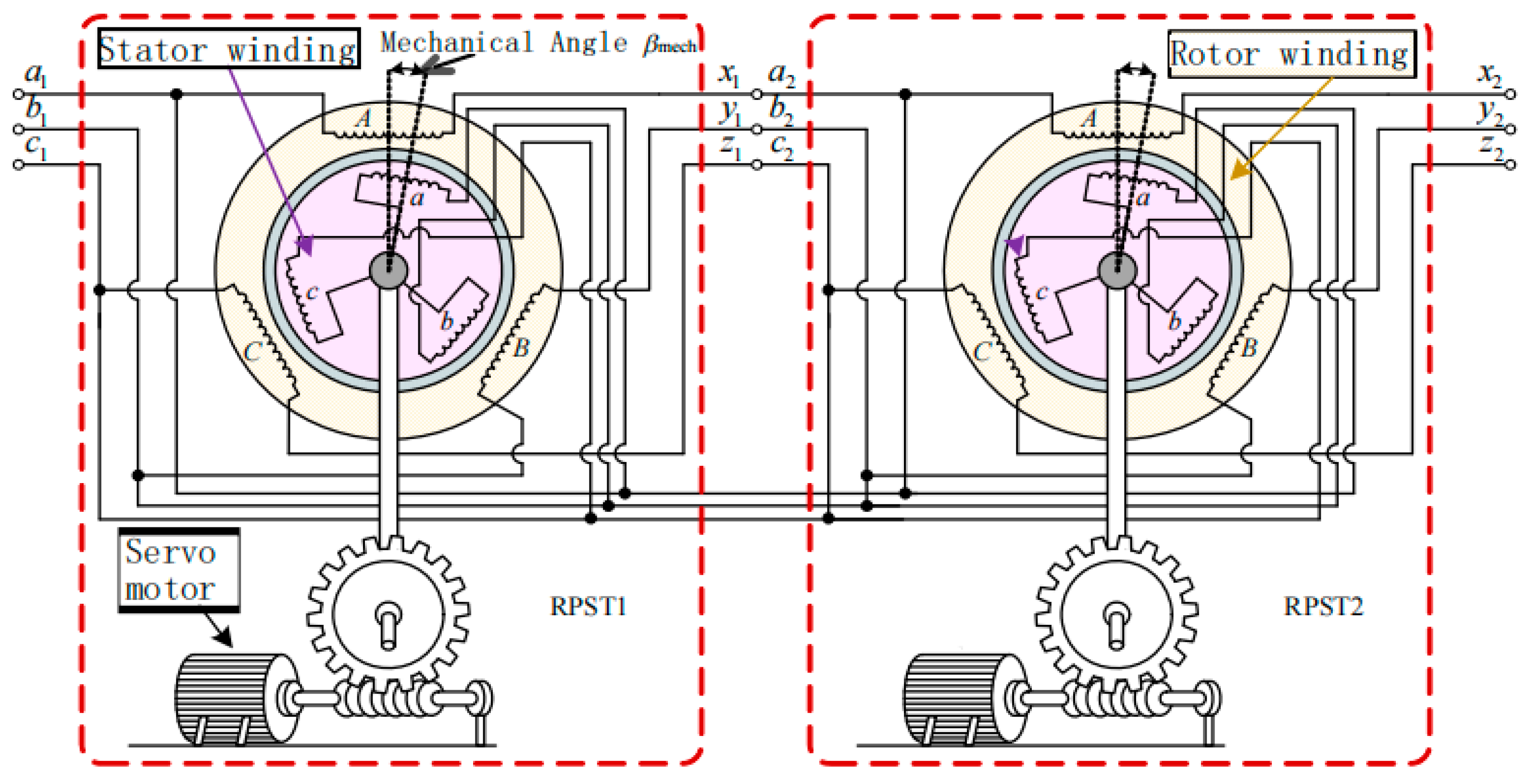
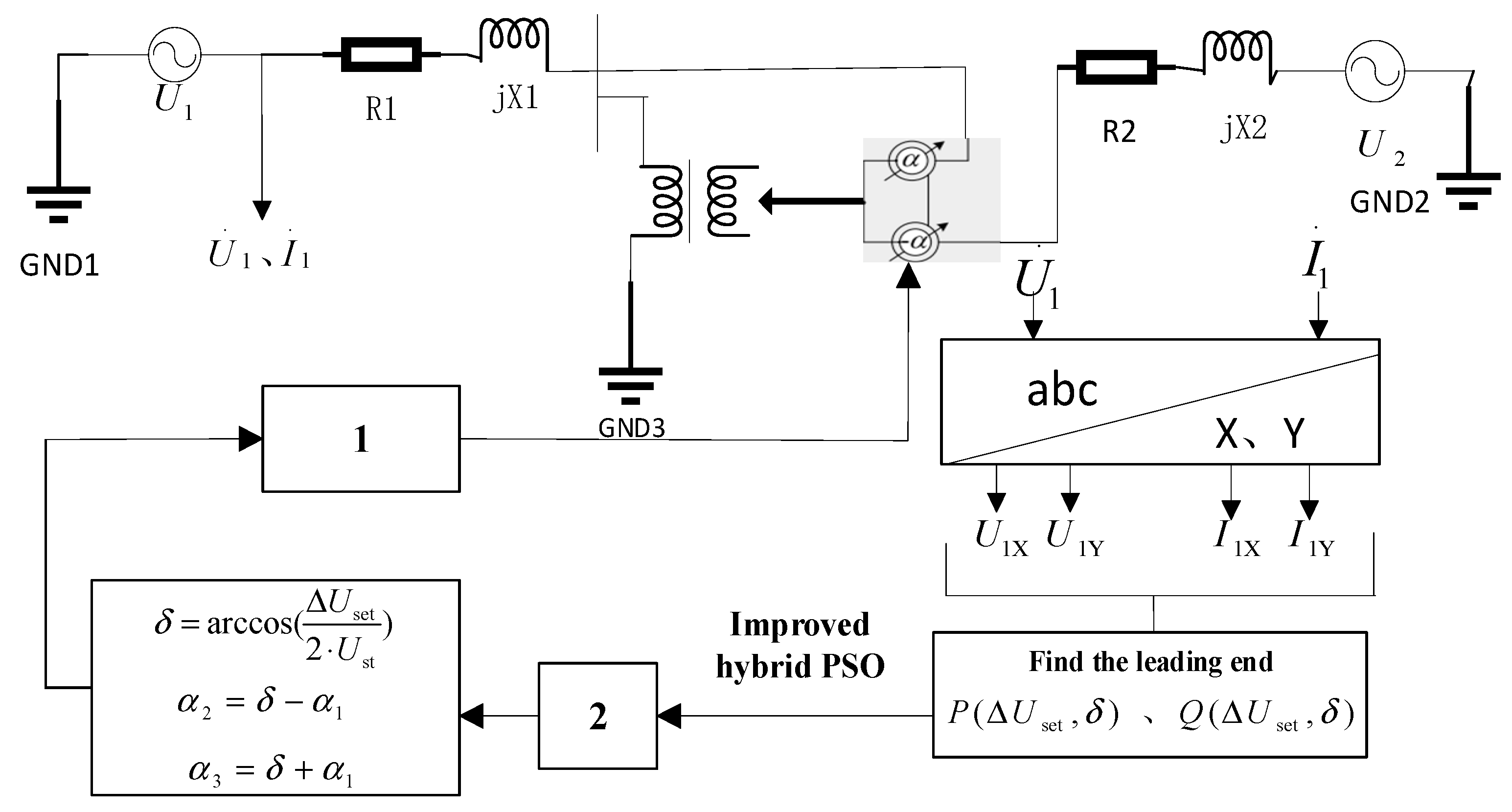
2.1. RPFC Topology [4]

An RPFC consists of two RPSTs; their topology is shown in Figure 1. Due to the large volume of the rotor winding coils, they are distributed on the outer side, while the stator is distributed on the inner side. A servo motor drives each RPST through gears. When the rotor rotates, there will be a mechanical phase difference between the stator and the rotor in phase, that is, the mechanical angle ${\beta }_{mesh}$. When integrating the stator and rotor with three phases in series into the electrical circuit, for a p-pole RPFC, when the rotor rotates a mechanical angle of ${\beta }_{mesh}$, its electrical angle changes by $p\ast {\beta }_{mesh}$.

Consequently, substantial phase adjustment of the device can be achieved by rotating the rotor through a minimal angle. This apparatus can be equivalently viewed as a controlled voltage source characterized by a specific magnitude and phase angle, which is connected in series with the line requiring regulation. This configuration allows for adjustments to the line voltage, thereby facilitating the adjustment of power flow through the line.

2.2. Operating Principle of RPFC [19]

Two RPSTs (Reactive Power Static Transformers) are used as voltage sources with a constant magnitude and continuously adjustable phase angles. Consequently, the voltage of the resultant RPFC (Reactive Power Flow Controller) exhibits a continuously adjustable phase and magnitude within a 360-degree range, functioning in the circuit as a controlled voltage source. The internal resistance of this controlled voltage source can be equivalently represented as a line impedance, as illustrated in Figure 2.

Let $\delta$ be the angle between the RPFC output voltage and the stator voltage, $\Delta U_{\mathrm{set}}$ be its amplitude, $U_{\mathrm{st}}$ be the RPST voltage amplitude, and $U_0$ be the stator voltage, as illustrated in Figure 3.

${\alpha }_1$ is the angle between $U_{\mathrm{st}}$ and $\Delta U_{\mathrm{set}}$, then:

$$\delta =\arccos ({\displaystyle \frac{\Delta U_{\mathrm{set}}}{2·U_{\mathrm{st}}}})$$

(1)

The angle between the two RPSTs and the stator voltage is as follows:

$${\alpha }_2=\delta -{\alpha }_1$$

(2)

$${\alpha }_3=\delta +{\alpha }_1$$

(3)

Then, the size of ${\alpha }_2$ and ${\alpha }_3$ in the circuit can be modified to adjust $\Delta U_{\mathrm{set}}$ and $\delta$, changing the output voltage amplitude and phase angle of the RPFC in the circuit.

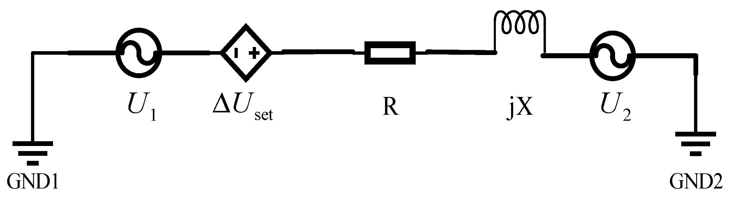
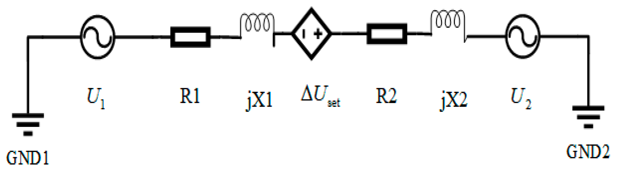
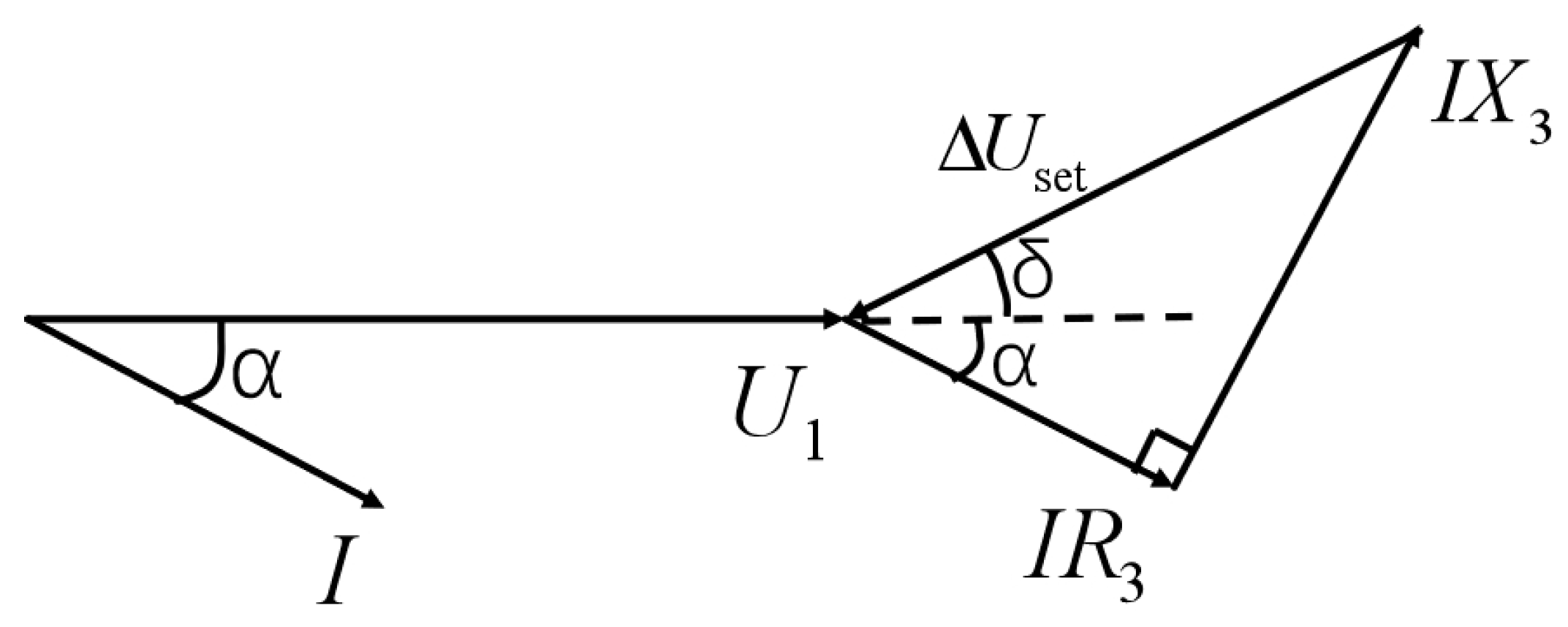
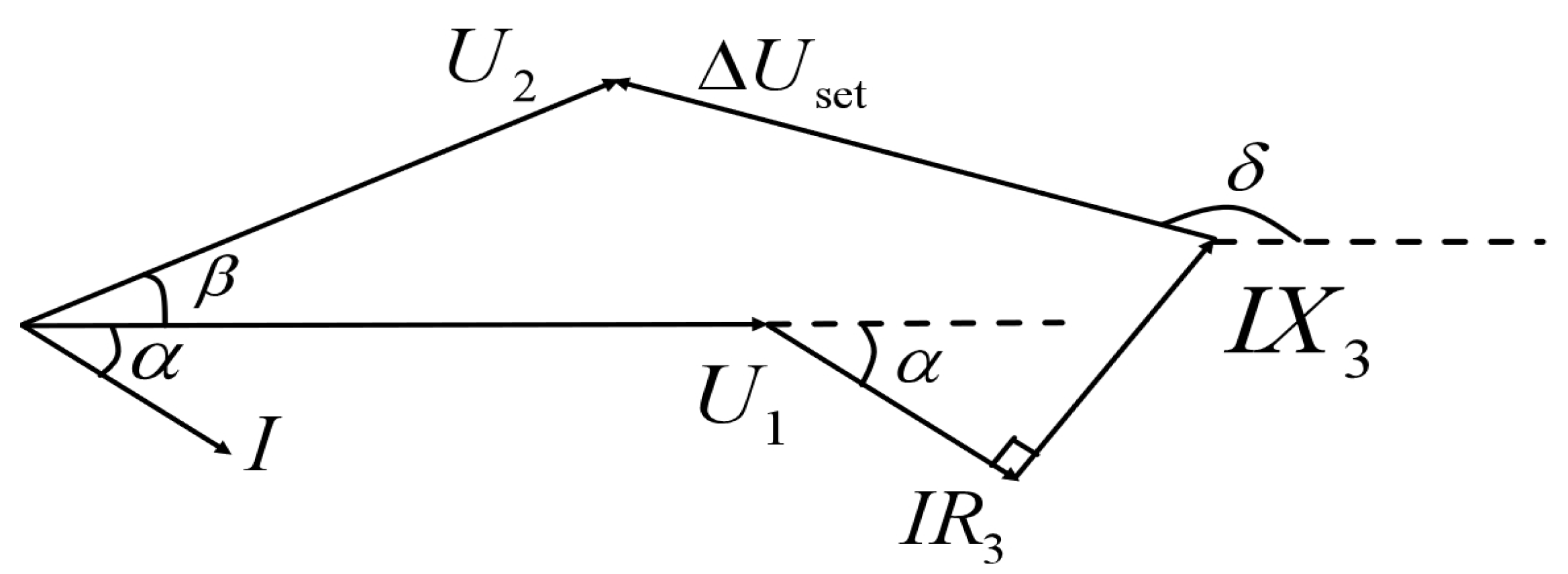
2.3. Establishment of the Model and Derivation of the Power Expression

The mathematical model of an RPFC is shown in Figure 3. The line voltage magnitudes of $U_1$ and $U_2$ are those of the voltage sources with adjustable phases at both ends and identical magnitudes. $R_1+j{X}_1$ is the line impedance, $\Delta U_{\mathrm{set}}$ is the amplitude of the RPFC equivalent controlled voltage source, and $R_2+j{X}_2$ is the internal impedance of the RPFC. Compared to traditional grid-connected models of RPFCs, this study considers both the line impedance and the internal impedance of the RPFC on an original basis. Due to the decoupling of the power, previous related research necessitated neglecting the relevant impedance values, resulting in deviations between the model and actual conditions. In addition, $\alpha$ is the angle between the terminal voltage $U_1$ and the line current $I$, while $R_3$ and $X_3$ are the equivalent total resistance and reactance in the line, respectively. Finally, $\delta$ is the angle between $U_1$ and the RPFC output voltage $\Delta U_{\mathrm{set}}$.

(1)

On the basis of Figure 4, we can draw the phase diagram of the line voltage and current when the angle between $U_1$ and $U_2$ is $0^{°}$, as shown in Figure 5 (with a reference phase angle of $U_1$).

The phasors can be decomposed in the graph, as follows:

$$\Delta U_{\mathrm{set}}·\sin (\delta )=I{X}_3\cos (\alpha )-I{R}_3\sin (\alpha )$$

(4)

$$\Delta U_{\mathrm{set}}·\cos (\delta )=I{R}_3\cos (\alpha )+I{X}_3\sin (\alpha )$$

(5)

The transformation indicates that electric current has the following:

$$I={\displaystyle \frac{\Delta u_{\mathrm{set}}\cos (\delta )}{R_3\cos (\alpha )+X_3\sin (\alpha )}}={\displaystyle \frac{\Delta u_{\mathrm{set}}\sin (\delta )}{X_3\cos (\alpha )-R_3\sin (\alpha )}}$$

(6)

From the impedance triangle in Figure 4:

$$\tan (\alpha +\delta )={\displaystyle \frac{X_3}{R_3}}$$

(7)

The transformation has the following:

$$\alpha +\delta =\arctan {\displaystyle \frac{X_3}{R_3}}$$

(8)

$$\alpha =\arctan ({\displaystyle \frac{X_3}{R_3}}-\delta )$$

(9)

The route power flow calculation formula has the following:

$$P=\sqrt{3}{U}_{1}I\cos (\alpha )=\sqrt{3}{U}_1{\displaystyle \frac{\Delta U_{\mathrm{set}}\cos (\delta )\cos (\alpha )}{R_3\cos (\alpha )+X_3\sin (\alpha )}}$$

(10)

$$Q=\sqrt{3}{U}_{1}I\sin (\alpha )=\sqrt{3}{U}_1{\displaystyle \frac{\Delta U_{\mathrm{set}}\cos (\delta )\sin (\alpha )}{R_3\cos (\alpha )+X_3\sin (\alpha )}}$$

(11)

When Formula (7) is substituted into Formula (8), Formula (9) has the following:

$$P={\displaystyle \frac{\sqrt{3}{U}_1\Delta U_{\mathrm{set}}\cos (\delta )\cos (\arctan \frac{X_3}{R_3}-\delta )}{R_3\cos (\arctan \frac{X_3}{R_3}-\delta )+X_3\sin (\arctan \frac{X_3}{R_3}-\delta )}}$$

(12)

$$Q={\displaystyle \frac{\sqrt{3}{U}_1\Delta U_{\mathrm{set}}\cos (\delta )\sin (\arctan \frac{X_3}{R_3}-\delta )}{R_3\cos (\arctan \frac{X_3}{R_3}-\delta )+X_3\sin (\arctan \frac{X_3}{R_3}-\delta )}}$$

(13)

(2)

In accordance with Figure 5, the line voltage and current phasor diagram can be drawn when the angle between $U_1$ and $U_2$ is $\beta$, as shown in Figure 6 (with $U_1$ as the reference phasor).

The phasors can be decomposed in the graph as follows:

$$U_1+I{R}_3\cos (\alpha )+I{X}_3\sin (\alpha )-\Delta U_{\mathrm{set}}\cos (\pi -\delta )=U_2\cos (\beta )$$

(14)

$$I{X}_3\cos (\alpha )+\Delta U_{\mathrm{set}}\sin (\pi -\delta )-I{R}_3\sin (\delta )=U_2\sin (\beta )$$

(15)

Through transformation:

$$I\cos (\alpha )={\displaystyle \frac{1}{R^2+X^2}}[U_2(R\cos (\beta )+X\sin (\beta ))-\Delta U_{set}(R\cos (\delta )+X\sin (\delta ))-U_{1}R]$$

(16)

From the calculation formula of the active current of the line:

$$P=\sqrt{3}{U}_{1}I\cos (\alpha )={\displaystyle \frac{\sqrt{3}{U}_1}{R^2+X^2}}[U_{2}R\cos (\beta )+U_{2}X\sin (\beta )-\Delta U_{set}(R\cos (\delta )+X\sin (\delta ))-U_{1}R]$$

(17)

Similarly, the line of the reactive power trend has the following:

$$Q=\sqrt{3}{U}_{1}I\sin (\alpha )={\displaystyle \frac{\sqrt{3}{U}_1}{R^2+X^2}}[U_{2}X\cos (\beta )-U_{2}R\sin (\beta )+\Delta U_{set}(R\sin (\delta )-X\cos (\delta ))-U_{1}R]$$

(18)

3. Power Separate Control

3.1. Power Separate Control Strategy (Taking the Case Where the Phases of $U_1$ and $U_2$ Are Identical as an Example)

From Formulas (12) and (13), when $U_1$, $X_3$ and $R_3$ are known, P and Q can be represented by a function with $∆U_{set}$ and $\delta$ as independent variables. However, when the target values of P and Q are known, it is not feasible to convert Equations (12) and (13) into explicit functions through equation-solving methods to obtain precise values for $∆U_{set}$ and $\delta$. Consequently, a regulatory strategy cannot be formulated based on this approach. Therefore, using the method of obtaining numerical solutions to derive approximate solutions is necessary to determine the adjustment routes of P and Q.

In this paper, an enhanced hybrid particle swarm optimization algorithm is employed to find the numerical solutions for the independent variables $∆U_{set}$ and $\delta$ given the known active and reactive powers [20]. To enhance robustness and reduce the potential for oscillations and fluctuations, the target power and known power are divided into more than 15 equal segments, and segmented regulation is implemented. Leveraging the multi-objective optimization capability of the PSO algorithm, the optimal path for active power regulation is first sought under the condition of constant reactive power. Subsequently, the optimal path for reactive power regulation is determined with the active power held constant. This approach achieves separate control of the active and reactive powers.

The particle swarm optimization (PSO) algorithm is a biomimetic approach that mimics the migratory and flocking behaviors observed in bird feeding processes. The process can be described as follows: the distance between individuals and food is known. Still, the food’s location is unknown; individuals continuously share information about the nearest known position to the food within the group. Upon receiving this shared information, each individual adjusts its flight direction and position. Through continuous adjustments of their flight trajectories and exchanges of group information, each bird in the population can locate the food as quickly as possible. Abstracted into a corresponding algorithm, this involves randomly generating N particles in a D-dimensional solution space. Each is assigned an initial velocity and position. By acquiring self-awareness of their own states, sharing information, and cooperating with the rest of the population, particles continuously adjust their iterative trajectories to pursue both individual and global extrema, ultimately finding the optimal solution within the solution space. The formula for updating particle states is as follows:

$${v_i}^{k+1}=w·{v_i}^k+c_1·ran{d_1}^k({P_i}^k-{X_i}^k)+c_2\ast ran{d_2}^k({P_g}^k-{X_i}^k)$$

(19)

$${X_i}^{k+1}={X_i}^k+{v_i}^{k+1}$$

(20)

where $w$ is the inertia weight; $c_1$ and $c_2$ are learning factors; and ${X_i}^k$ and ${v_i}^k$ are the positions and velocities of particle i in the kth iteration. ${X_i}^k=({X_{i1}}^k,{X_{i2}}^k,\cdots ,{X_{iD}}^k)$, ${v_i}^k=({v_{i1}}^k,{v_{i2}}^k,\cdots ,{v_{iD}}^k)$, and $i=1,2,3,\cdots ,N$, ${P_i}^k$ and ${P_g}^k$ are the individual extreme values of the kth iteration and global extreme values of the population, ${P_i}^k=({P_{i1}}^k,{P_{i2}}^k,\cdots ,{P_{iD}}^k)$, $i=1,2,3,\cdots ,N$, and ${P_g}^k=({P_{g1}}^k,{P_{g2}}^k,\cdots ,{P_{gD}}^k)$.

The particle swarm optimization (PSO) algorithm boasts simplicity in principle, a minimal number of parameters, ease of implementation, and a degree of versatility. However, it also exhibits certain defects and shortcomings in practical applications. Firstly, as each particle “flies” towards the optimal solution based on the collective and individual search experiences of all particles, under the influence of large inertia factors, particles may lack a refined search for the optimal solution, leading to insufficient search accuracy. Secondly, as all particles “fly” towards the optimal solution, their velocities decrease as they approach the optimal particle, causing the particle swarm to converge towards uniformity and lose diversity among particles. This results in a significant slowdown in the convergence speed of the algorithm during the later stages of evolutionary iteration and susceptibility to premature convergence, trapping the algorithm in a local optimal solution.

Due to the defects in the iteration rate and convergence rate and the ease of falling into the local optimum, this paper improves the optimization process and then uses it for power regulation work.

First, the logistic chaotic map is used to initialize the population of particles, such that the initial particles are evenly distributed in the search interval and guaranteed not to fall into a local optimum as much as possible.

Second, crossover and variation are added to the genetic algorithm. A random number between 0 and 1 is generated after each iteration. If the random number is greater than the predetermined crossover probability, then the crossover step is skipped; otherwise, a certain number of parents choose the size of the set crossover pool and execute the next instruction instead of the original parent.

The position of the offspring may be expressed as:

$$c{h}_{(\mathrm{x})}=q·par{1}_{(\mathrm{x})}+(1-q)·par{2}_{(\mathrm{x})}$$

(21)

Perhaps:

$$c{h}_{(\mathrm{x})}=q·par{2}_{(\mathrm{x})}+(1-q)·par{1}_{(\mathrm{x})}$$

(22)

and q is a random number between 0 and 1.

The velocity of the offspring can be expressed as:

$$c{h}_{(\mathrm{v})}={\displaystyle \frac{par{1}_{(\mathrm{v})}+par{2}_{(\mathrm{v})}}{\left|par{1}_{(\mathrm{v})}+par{2}_{(\mathrm{v})}\right|}}·\left|par{1}_{(\mathrm{v})}\right|$$

(23)

Perhaps:

$$c{h}_{(\mathrm{v})}={\displaystyle \frac{par{1}_{(\mathrm{v})}+par{2}_{(\mathrm{v})}}{\left|par{1}_{(\mathrm{v})}+par{2}_{(\mathrm{v})}\right|}}·\left|par{2}_{(\mathrm{v})}\right|$$

(24)

Then, a number between 0 and 1 is randomly generated similarly. If this number exceeds the preset probability of mutation, the mutation operation is skipped, and the next step is executed. Meanwhile, the quantitative parent is randomly selected with the preset mutation proportion, and the Cauchy distribution is used to change the position and make it the new position.

The variation formula is as follows:

$$x^{\prime }=x+{\displaystyle \frac{x}{\pi ·(1+x^2)}}$$

(25)

where x is the position before the mutation, and x′ is the new position after the mutation.

Due to space limitations, and as the focus of this paper is not on algorithm improvements, for detailed enhancements and performance comparisons of the hybrid particle swarm optimization algorithm relative to the standard particle swarm optimization algorithm, please refer to Ref. [20].

The flowchart for power regulation using the hybrid particle swarm optimization algorithm (Figure 7) compared to the standard particle swarm optimization algorithm (Figure 8) is as follows (using the adjustment of active power control while the reactive power remains unchanged as an example):

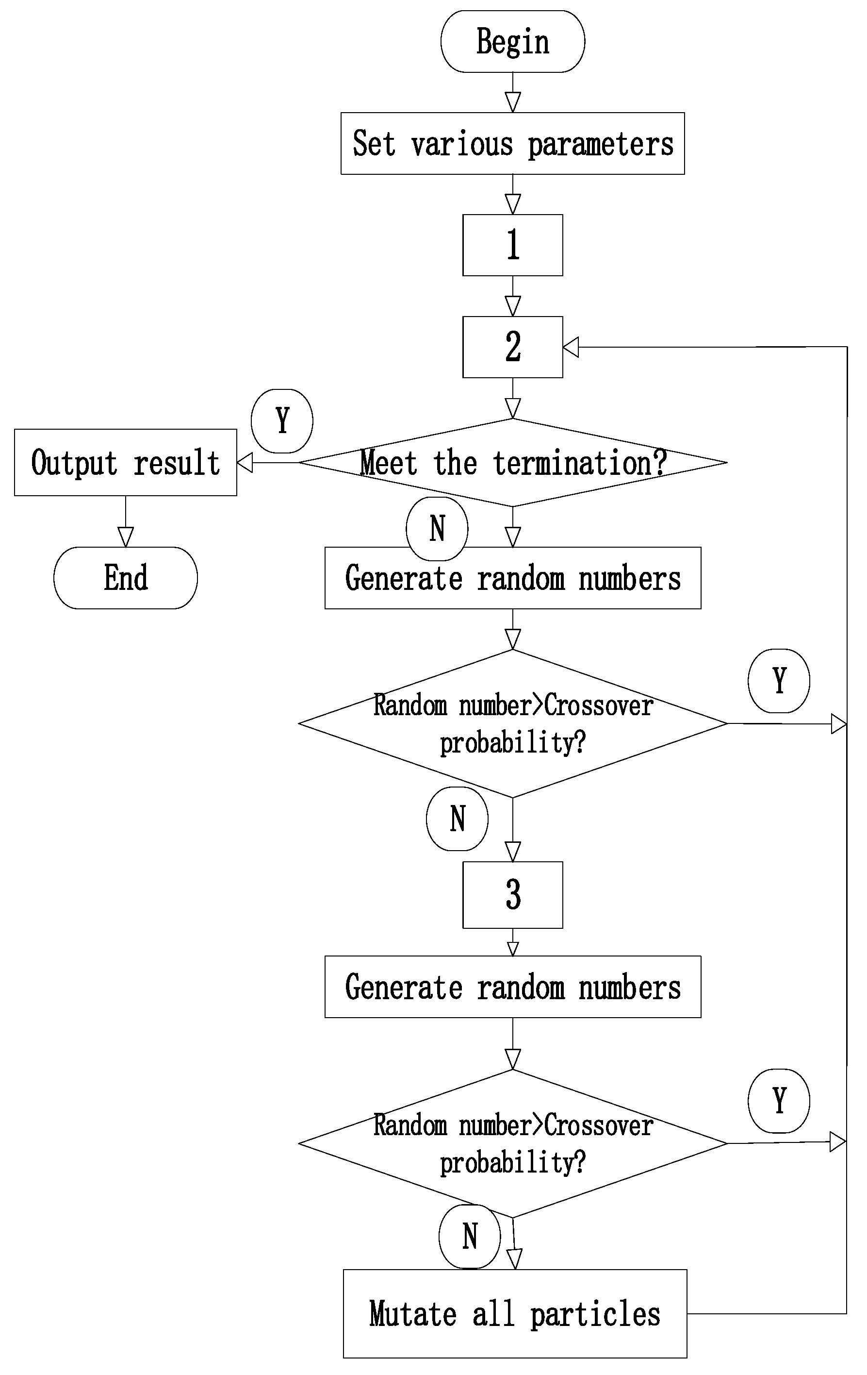
• The active and known values are divided into n (n > 10) paragraphs. The objective function is set to a constant reactive power, and the active power is adjusted in stages. Initialization of the particle population is carried out by logistic chaotic mapping.
• Each particle’s position, velocity, and fitness are calculated, and the global variables are updated.
• The parent particles are selected to cross with the set cross pool size, and the parent particles are replaced.

The code debugging results can show the value of the independent variable at the beginning and end of each paragraph, and the resulting value, which is adjustable, can be imported into the simulation.

Please refer to Figure 9 for the specific process of power regulation.

• Two phase shifters are executed to rotate the path.
• If P is adjusted, Q, the voltage amplitude, and the phase change path are unchanged; if Q and P are unchanged, the voltage amplitude and phase change path are adjusted.

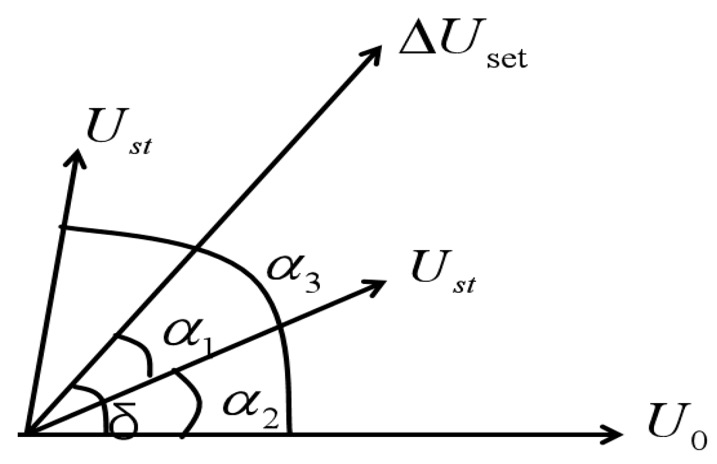
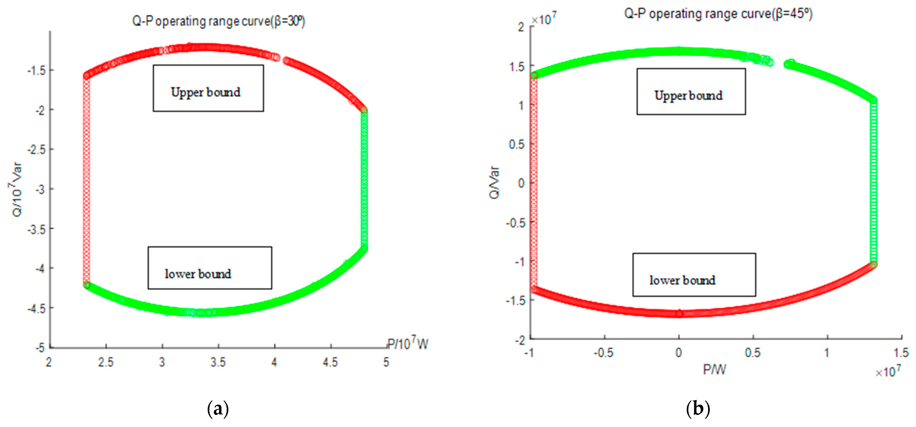
3.2. Q–P Operating Range Curve Construction (Using the Angle Between U₁ and U₂ as an Example of β)

The algorithm described in Section 3.1 can first calculate the active power range and then take sufficient points from it. The algorithm calculates the active power’s maximum and minimum values, which remain constant. The operating range curve is drawn with Q as the vertical axis variable and P as the horizontal axis variable.

4. Simulation Verification

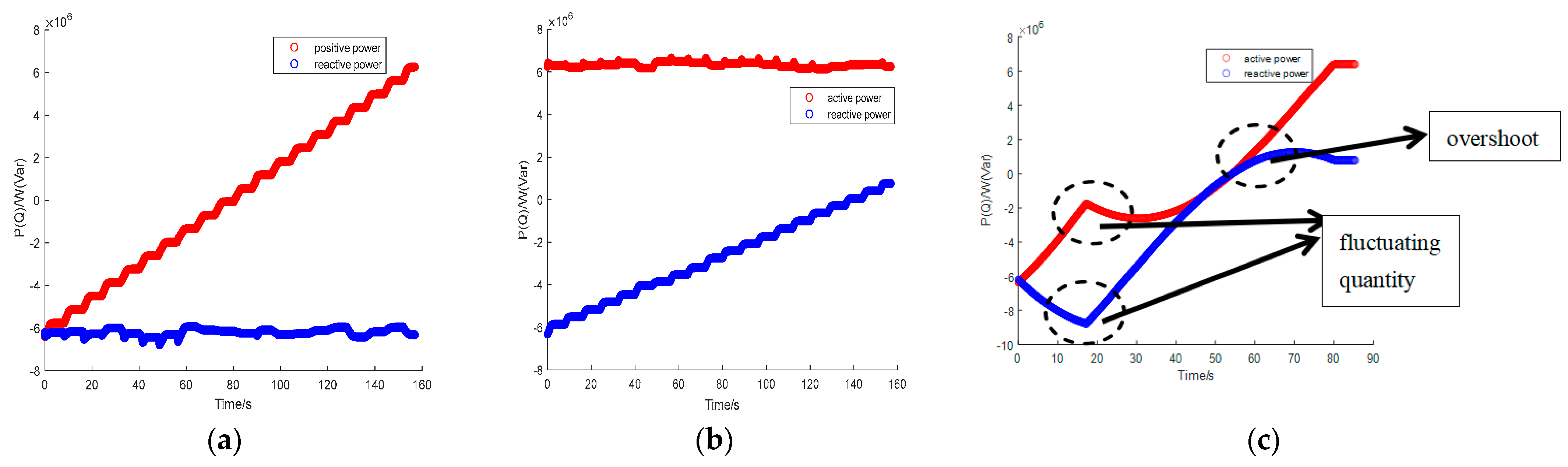
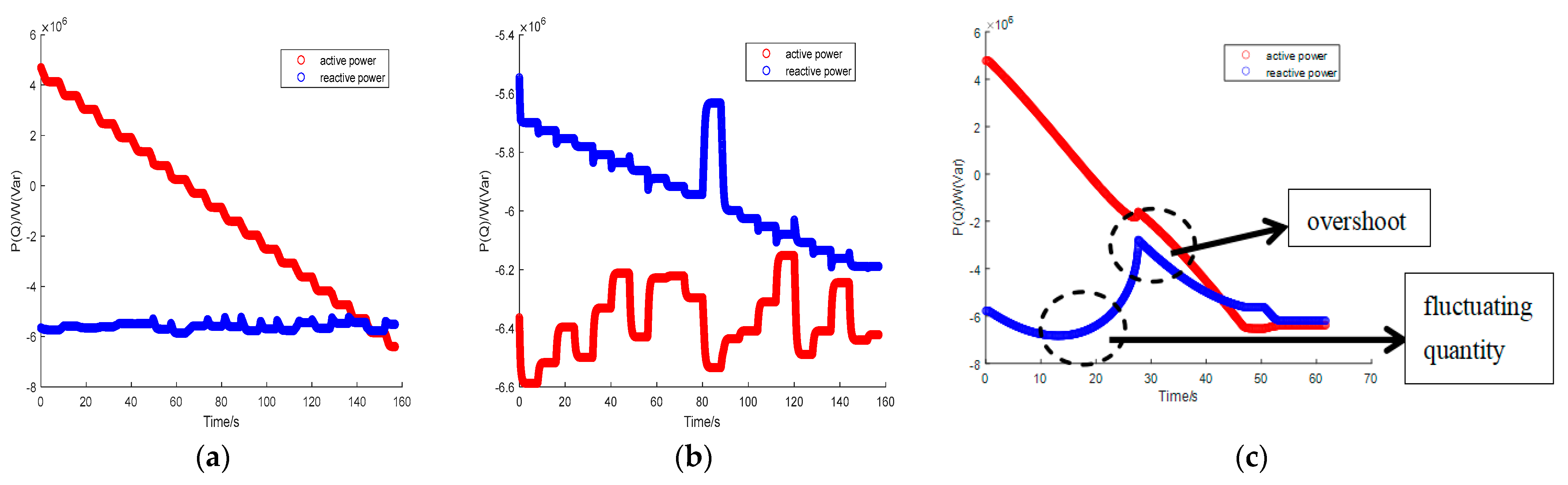
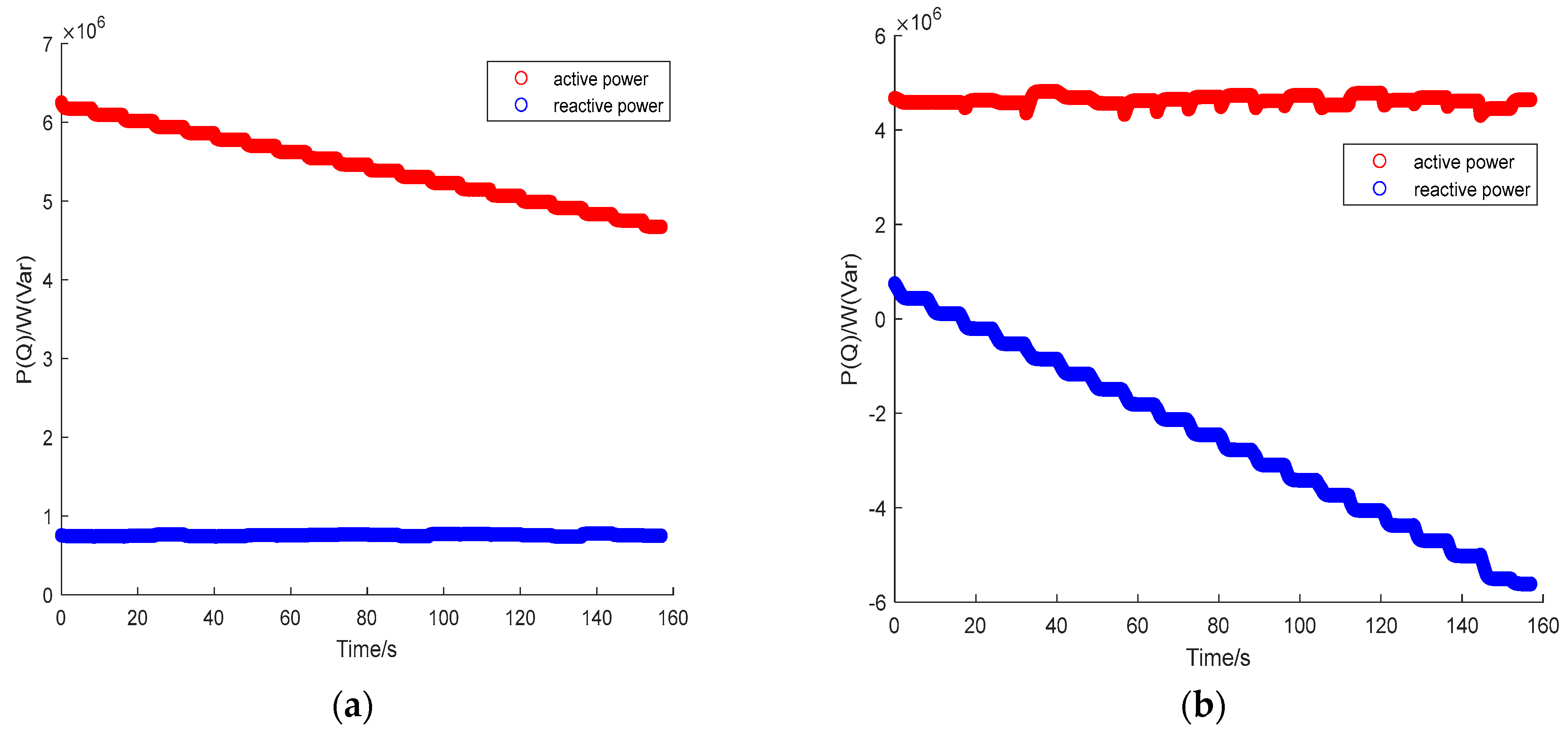
4.1. Voltage In-Phase Line Simulation of 10 kV

(1)

The initial vision in power is as follows:

$$\tilde{S}=P_1+j{Q}_1=-6.4373·{10}^6-\mathrm{j}6.2463·{10}^6\mathrm{VA}$$

The target is viewed in power as follows:

$$\widetilde{S_2}=P_2+j{Q}_2=6.2869·{10}^6+\mathrm{j}7.5010·{10}^5\mathrm{VA}$$

(2)

The initial vision in power is as follows:

$$\widetilde{S_1}=P_1+j{Q}_1=4.6993·{10}^6-\mathrm{j}5.6991·{10}^6\mathrm{VA}$$

The target is viewed in power as follows:

$${\tilde{S}}_2=P_2+j{Q}_2=-6.4373·{10}^6-\mathrm{j}6.2463·{10}^6\mathrm{VA}$$

(3)

The initial vision in power is as follows:

$$\widetilde{S_1}=P_1+j{Q}_1=6.2869·{10}^6+\mathrm{j}7.5010·{10}^5\mathrm{VA}$$

The target is viewed in power as follows:

$$\widetilde{S_2}=P_2+j{Q}_2=4.6993·{10}^6-\mathrm{j}5.6991·{10}^6\mathrm{VA}$$

This section simulates a 10 kV single circuit line in MATLAB/Simulink and compares the improved algorithm control strategy proposed in this paper with one-step adaptive regulation through simulation examples. The specific parameters of the line are shown in

Table 1. Parameters for the simulation of a line with in-phase voltages at both ends of a 10 kV system.

Parameter	Numeric Value
The voltage at the first end of the line $U_1/\mathrm{kV}$	$10$
Line end voltage $U_2/\mathrm{kV}$	$10$
Line impedance $R_1+\mathrm{j}{X}_1/\mathsf{\Omega }$	$0.48+\mathrm{j}0.60$
RPFC intrinsic impedance $R_2+\mathrm{j}{X}_2/\mathsf{\Omega }$	$0.025+\mathrm{j}0.44$
RPFC voltage adjustable range/V	$0–1600$
RPFC with adjustable angle/°	$0–360$

. Please see Figure 10, Figure 11 and Figure 12 for the simulation image results. Compared with traditional control strategies, the control strategy proposed in this paper takes longer. According to experimental data, the adjustment employing adaptive algorithms necessitates approximately 85 s in Figure 10 and roughly 64 s in Figure 11, whereas the tuning approach proposed in this paper requires approximately 160 s. This translates to an average increase of approximately 100 s compared to the adaptive algorithms. However, the control effect on the power that should not change during the adjustment process is relatively good, and it can often be controlled within a small fluctuation range. In the above three experiments, the power that should not be changed can be controlled within a fluctuation range of 5%. The hybrid particle swarm algorithm has small fluctuations and no excessive overshoot during the adjustment process for the power that needs to be adjusted. It is adjusted step by step according to the design in Section 3.1, ensuring good stability and robustness. The original adaptive adjustment method can be applied as depicted in Figure 10c and Figure 11c. The trend of medium power variation shows significant fluctuations in certain areas, resulting in a 10% to 20% overshoot during the regulation process. When decoupling the power, the original adaptive adjustment strategy neglects the line resistance, facilitating the decoupling process. However, during the practical line simulations, this neglect of the line resistance led to discrepancies with actual conditions at certain moments during the adjustment [4], resulting in overshoots. In contrast, this paper constructed the power equations based on actual line conditions and performed power adjustment separately, making the simulations closer to reality. Consequently, the adjustment process exhibited reduced overshoots. The existence of these overshoots is not conducive to maintaining system stability during power regulation, and significant fluctuations can have some impact on corresponding devices and equipment. Therefore, compared with the original adaptive control method, the control strategy proposed in this study has stronger stability and robustness.

4.2. Q-P Operating Range Curve of 10 kV

Based on this algorithm, an image of the power operating range at different voltage phases at both ends can be drawn (Figure 13). The specific parameters of the line are shown in

Table 2. Parameters for a 10 kV line with out-of-phase voltages at both ends.

Parameter	Numeric Value
The voltage at the first end of the line $U_1/\mathrm{kV}$	$10$
Line end voltage $U_2/\mathrm{kV}$	$10$
Line impedance $R_1+\mathrm{j}{X}_1/\mathsf{\Omega }$	$0.48+\mathrm{j}0.6$
RPFC intrinsic impedance $R_2+\mathrm{j}{X}_2/\mathsf{\Omega }$	$0.025+\mathrm{j}0.44$
RPFC voltage adjustable range/V	$0–1600$
RPFC with adjustable angle/°	$0–360$

. The operating range is surrounded by two vertical lines on the left and right and two arcs on the top and bottom. In practical engineering applications, technicians can draw the corresponding power operating range images using this method, identifying the adjustable power range and effectively adjusting the actual line power.

5. Conclusions

In this study, the voltage and current are decomposed, and the formula of the first end power is derived. Then, an improved hybrid PSO can adjust the part between the initial and target power. This algorithm can be used to construct the Q–P running diagram. The following conclusions are drawn:

• This paper introduces intelligent optimization algorithms into the power regulation control strategy for Rotating Power Flow Controllers (RPFCs) for the first time. Through simulations, it was found that the proposed strategy can effectively meet the objectives of independent regulation of the active and reactive powers, providing a potential pathway for pursuing more precise power regulation in the future.
• Compared with adaptive adjustment strategies, the strategy proposed in this paper considers all factors related to the transmission line without the need for neglect due to decoupling requirements. Therefore, it aligns more closely with actual conditions during the adjustment process, resulting in smaller power overshoots and fluctuations. However, due to the relatively basic nature of the algorithm, the adjustment duration is longer. In the future, more advanced algorithms from the field of artificial intelligence can be utilized to improve the adjustment rate.
• The control strategy proposed in this paper allows for plotting the Q-P operating range diagram for line power flow. In practical engineering, technicians can refer to these diagrams to avoid target powers that do not align with actual conditions, thereby enhancing the adjustment efficiency. In the future, relevant algorithms can be employed to calculate relevant parameters during the power adjustment process of RPFCs, improving the execution efficiency of power regulation.

References

1. Liu, J.L.; Liu, X.M.; Lu, X. Analysis methods and countermeasures for supply-demand balance of high proportion new energy systems. High Volt. Technol. 2023, 49, 2711–2724. [Google Scholar]
2. Ma, W.M. Some Thoughts on the Development of Frontier Technologies in Electrical Engineering. J. Electr. Eng. 2021, 36, 4627–4636. [Google Scholar]
3. Zhou, X.X.; Chen, S.Y.; Lu, Z.X. Technical Characteristics of China’s New Generation Power System in Energy Transition. Chin. J. Electr. Eng. 2018, 38, 1893–1904+2205. [Google Scholar]
4. Yan, X.W.; Peng, W.F.; Jia, J.X. Research on Power Regulation Method of Rotary Power Flow Controller Based on Adaptive Control of Rotation Speed. Proc. Chin. Soc. Electr. Eng. 2023, 43, 4971–4987. [Google Scholar]
5. Li, S.; Tang, F.; Liu, D.C. Study on the Efficiency of Distributed Power Flow Controllers in Improving Maximum Transmission Capacity Expectations and Power Supply Reliability. Grid Technol. 2018, 42, 1573–1580. [Google Scholar]
6. Fujita, H.; Hara, S.; Piwko, K.J. Simulator model of rotary power flow controller. In Proceedings of the 2001 Power Engineering Society Summer Meeting, Vancouver, BC, Canada, 15–19 July 2001; pp. 1794–1797. [Google Scholar]
7. Larsen, E.V. Power Flow Control with Rotary Transformers. U.S. Patent 5,841,267, 24 November 1998. [Google Scholar]
8. Larsen, E.V. Power Flow Control and Power Recovery with Rotary Transformers. U.S. Patent 5,953,225, 14 September 1999. [Google Scholar]
9. Fardanesh, B.; Schuff, A. Dynamic Studies of the NYS transmission system with the marcy csc in the UPFC and IPFC configurations. In Proceedings of the 2003 IEEE PES Transmission and Distribution Conference and Exposition, Dallas, TX, USA, 7–12 September 2003; pp. 1126–1130. [Google Scholar]
10. Kim, S.Y.; Yoon, J.S.; Chang, H.B. The operation experience of KEPCO UPFC. In Proceedings of the Intermational Conference on Electrical Machines and Systems (ICEMS 2005), Nanjing, China, 27–29 September 2005; pp. 1–4. [Google Scholar]
11. Qi, W.C.; Yang, L.; Song, P.C. UPFC system control strategy research in Nanjing western power grid. Power Syst. Technol. 2016, 40, 92–96. [Google Scholar]
12. Ba, A.O.; Peng, T.; Lefebvre, S. Rotary Power-Flow Controller for Dynamic Performance Evaluation—Part I: RPFC Modeling. IEEE Trans. Power Deliv. 2009, 24, 1406–1416. [Google Scholar] [CrossRef]
13. Haddadi, A.M.; Kazemi, A. Optimal power flow control by rotary power flow controller. Adv. Electr. Comput. Eng. 2011, 11, 79–86. [Google Scholar] [CrossRef]
14. Ba, A.O.; Peng, T.; Lefebvre, S. Rotary Power-Flow Controller for Dynamic Performance Evaluation—Part II: RPFC Application in a Transmission Corridor. IEEE Trans. Power Deliv. 2009, 24, 1417–1425. [Google Scholar] [CrossRef]
15. Tan, Z.L.; Zhang, C.P.; Jiang, Q.R. Comparison of Rotary Power Flow Controller and Unified Power Flow Controller with Sen Transformer. Power Syst. Technol. 2016, 40, 868–874. [Google Scholar]
16. Tan, Z.L.; Zhang, C.P.; Jiang, Q.R. Study on Steady-state Characteristics of Rotary Power Flow Controller. Power Syst. Technol. 2015, 39, 1921–1926. [Google Scholar]
17. Tan, Z.L.; Zhang, C.P.; Jiang, Q.R. Research on characteristics and power flow control strategy of rotary power flow controller. In Proceedings of the 2015 5th International Youth Conference on Energy (IYCE), Pisa, Italy, 27–30 May 2015; pp. 1–8. [Google Scholar]
18. Jia, J.X.; Peng, W.F.; Yan, X.W. Decoupling Control Method of Rotary Power Flow Controller Based on Cosine Theorem. J. Electr. Eng. Technol. 2023, 38, 3425–3435. [Google Scholar]
19. Yan, X.W.; Peng, W.F.; Shao, C. Voltage Regulation Method of User Side Based on Rotary Power Flow Controller. J. Electr. Eng. Technol. 2023, 38 (Suppl. S1), 70–79+113. [Google Scholar]
20. Zhang, Z.Y.; Jia, J.X.; Lu, J.D. Optimal allocation of energy storage participating in peak shaving based on improved hybrid particle swarm optimization. In Proceedings of the 2023 IEEE 6th International Electrical and Energy Conference (CIEEC), Hefei, China, 12–14 May 2023; pp. 2245–2250. [Google Scholar]
Figure 1. Topology of an RPFC [4].
Mca 30 00020 g001
Figure 2. Equivalent circuit.
Mca 30 00020 g002
Figure 3. Relationship diagram between voltage and phase angle of RPFC.
Mca 30 00020 g003
Figure 4. Mathematical model of an RPFC.
Mca 30 00020 g004
Figure 5. Line voltage and current phasor diagram when the angle between U 1 and U 2 is 0 ° .
Mca 30 00020 g005
Figure 6. Line voltage and current phasor diagram when the angle between U 1 and U 2 is β .
Mca 30 00020 g006
Figure 7. Improved hybrid PSO tuning flowchart.
Mca 30 00020 g007
Figure 8. PSO tuning flowchart.
Mca 30 00020 g008
Figure 9. Decoupled regulation flowchart.
Mca 30 00020 g009
Figure 10. Power regulation image for Operating Condition (1).(a) The active power is adjusted, and reactive power control is maintained (improved hybrid PSO); (b) the reactive power is adjusted, and active power control is maintained (improved hybrid PSO); (c) adaptive adjustment method [4].
Mca 30 00020 g010
Figure 11. Power regulation image for Operating Condition (2). (a) The active power is adjusted, and reactive power control is maintained (improved hybrid PSO); (b) the reactive power is adjusted, and active power control is maintained (improved hybrid PSO); (c) adaptive adjustment method [4].
Mca 30 00020 g011
Figure 12. Power regulation image for Operating Condition (3). (a) The active power is adjusted, and reactive power control is maintained (improved hybrid PSO); (b) the reactive power is adjusted, and active power control is maintained (improved hybrid PSO).
Mca 30 00020 g012
Figure 13. (a) Two-end voltage angle β = 30°; (b) two-end point angle β = 45°.
Mca 30 00020 g013