Impact of Cooperation and Intra-Specific Competition of Prey on the Stability of Prey–Predator Models with Refuge

Abstract

The main objective of this study is to find out the influences of cooperation and intra-specific competition in the prey population on escaping predation through refuge and the effect of the two intra-specific interactions on the dynamics of prey–predator systems. For this purpose, two mathematical models with Holling type II functional response functions were proposed and analyzed. The first model includes cooperation among prey populations, whereas the second one incorporates intra-specific competition. The existence conditions and stability of different equilibrium points for both models were analyzed to determine the qualitative behaviors of the systems. Refuge through intra-specific competition has a stabilizing role, whereas cooperation has a destabilizing role on the system dynamics. Periodic oscillations were observed in both systems through Hopf bifurcation. From the analytical and numerical findings, we conclude that intra-specific competition affects the prey population and continuously controls the refuge class under a critical value, and thus, it never becomes too large to cause predator extinction due to food scarcity. Conversely, cooperation leads the maximal number of individuals to escape predation through the refuge so that predators suffer from low predation success.

1. Introduction

Prey–predator interaction has immense importance in the existence of life. In predator–prey systems, the prey population uses different defense mechanisms to escape from predators [1,2]. Among them, refuge is the most common in the literature [3,4], and it has become a significant issue in theoretical ecology [5,6,7]. One famous proverb about the Fox–Rabbit chase says, “The fox is only running for his dinner, but the rabbit is running for his life [8]”. If the rabbit can successfully save its life, it is called the rabbit escaping predation from the fox through refuge. Thus, the refuge can be defined as any strategy that decreases the rate of predation [9,10].

Refuge can be attained in two ways—(i) constant numerical refuge, where a definite number of individuals in the population escape from predation, and (ii) proportional refuge, where a fixed proportion of individuals in the population escape from predation. In both cases, the whole prey population cannot attain the facility of refuge, and thus, a particular number or fraction of the population is always exposed to the predator. If not, the predator population will no longer be able to persist, and the system will be destabilized.

If we consider a situation where a constant number of individuals in the population can enjoy the facility of refuge due to the availability of a fixed number of safe refuge places, two habitats are available for the prey population—either they live in the refuge habitat or they roam around in the open habitat where they are available to predators [11]. In [12], the authors considered a prey–predator model with a constant numerical prey refuge and showed that there are two major factors that control this type of refuge in the population: the population density of the prey (x) and the available refuge (M) (which is the maximum number of prey individuals that can be supported in the refuge habitat). When $x\le M$, competition among prey for refuge is negligible, since prey fitness depends only on predation [11]. Under such conditions, cooperation among individuals in the prey population must be seen. But, this is not the case at all times, because this type of refuge can include a definite number of individuals, and thus, they cannot move freely between habitats when the population size exceeds the refuge number ($x>M$), and obviously, intra-specific competition to take refuge will increase proportionally as the density increases. The conclusions regarding this type of refuge are that it has a strong stabilizing effect [13] and it can prevent the extinction of prey, but when the population is too large for all members to stay all in the refuge, coexistence with predators is expected, as the predators will obtain continuous resources [11]. So, in that case, the mortality rate of the prey increases when the population density goes beyond the refuge capacity, and this will cause a negative feedback stabilizing effect on the system [14].

In case of a proportional refuge, there are also two habitats available for the prey population– either they live in the refuge habitat or they roam around in the open habitat, where they are available to predators [11]. But, under such conditions, movement of prey individuals always occurs between the open and refuge habitats [15]. In [16], Kar proposed the Lotka–Volterra type prey–predator system, including proportional prey refuges, where m is denoted as the fractional refuge of prey from predators (which is different from the previously discussed refuge, M), and it ranges from $0<m<1$. Now, if we consider the whole prey population as x, then the $mx$ portion of the prey is in the refuge habitat, and the $(1-m)x$ portion of the prey is in open habitats and is thus available to the predators. For the proportional refuge, the whole population never has the opportunity to attain refuge, and thus, the process of finding a refuge place is either cooperation- or competition-based. This type of refuge can reduce the mortality rate of prey by reducing the predation pressure and can affect positively affect the growth of prey and negatively affect that of predators. Thus, in this way, refuge can act as a stabilizing effect in prey–predator dynamics [17]. Extreme refuge may destabilize prey–predator dynamics, as the predator population becomes extinct by suffering from lower predation success due to the large refuge size [18].

Mathematically, prey–predator interaction was first described by Alfred James Lotka in 1925 [19] and Vito Volterra in 1927 [20]. In 1934, Georgy Frantsevich Gause [21] first found refuge in his experiment with the protozoan predator Didinium feeding on Paramecium. One major drawback of the Lotka–Volterra model is that the predator population never becomes saturated. Crawford Stanley Holling solved this problem [22,23,24] by suggesting three kinds of functional responses (Holling types I, II, and III) for different species of predators. In 1963, Rosenzweig and MacArthur [25] first replaced the linear functional response of the Lotka–Volterra model with the Holling type II response function and first documented that prey–predator coexistence is not limited to a stable equilibrium; a limit cycle appears when the stable equilibrium undergoes Hopf bifurcation [26]. Since then, various modeling approaches for the prey–predator system, including refuge, have been conducted by researchers [16,27,28,29].

The stabilizing role of refuge in prey–predator systems was shown many years ago, and since then, various aspects of prey–predator systems with refuge have been analyzed using Holling type II nonlinearities [30,31]. Mapunda et al. [32] and Kumar et al. [30] showed the effect of intra-specific competition among predators on the prey–predator system in their respective studies. The effect of cooperation among predators on the prey–predator system through cooperative hunting strategies was shown by Saha and Samanta in their study [33]. The effect of inter-specific competition among predator populations in a three-species system was analyzed by Sarwadi et al. [29,34]. The impact of cooperation among two prey species in a three-species prey predator system was analyzed by Rihan et al. [35]. The present study fills the research gap by dealing with the impacts of cooperation and intra-specific competition among the prey population when escaping from predators through refuge on the prey–predator system, and it is found that when the prey individuals become competitive with each other for shelter in the refuge habitat, the system dynamics achieve stability faster. On the other hand, any cooperation among prey populations regarding refuge turns the stable equilibrium condition into a limit cycle condition.

In previous articles ([29,30,32,34] and the references therein), authors have considered competition among predator populations. To our knowledge, this is the first article to consider the impacts of cooperation and intra-specific competition within the prey population on attaining refuge. The key question of this study is “how are the dynamics of the prey–predator system impacted when the decision about refuge is made through cooperation and the same for intra-specific competition?” To obtain an answer to this problem, we developed two mathematical models. The first model includes cooperation among prey populations, whereas the second model contains intra-specific competition. The dynamics of the models were analyzed with qualitative theories.

This study is presented sequentially in the latter sections as follows: Section 2 deals with the mathematical model formation, including both the prey refuge and the cooperation among prey. The local stability and bifurcation analysis of the equilibrium points is provided. The global stability of the co-existing equilibrium is analyzed in Section 2.4. Another mathematical model considering the prey refuge and the intra-specific competition among prey is formed. The existence of Hopf bifurcation and a stability analysis are conducted in Section 3. The direction of Hopf bifurcation is analyzed in Section 3.4. Detail numerical simulations using Matlab are delineated in Section 4. The final discussion and biological interpretation of the results are included in the conclusions in Section 5.

2. Mathematical Model for Prey Refuge and Cooperation

Here, we propose the Lotka–Volterra type prey–predator system, including proportional prey refuge and cooperation, which makes the following assumptions:

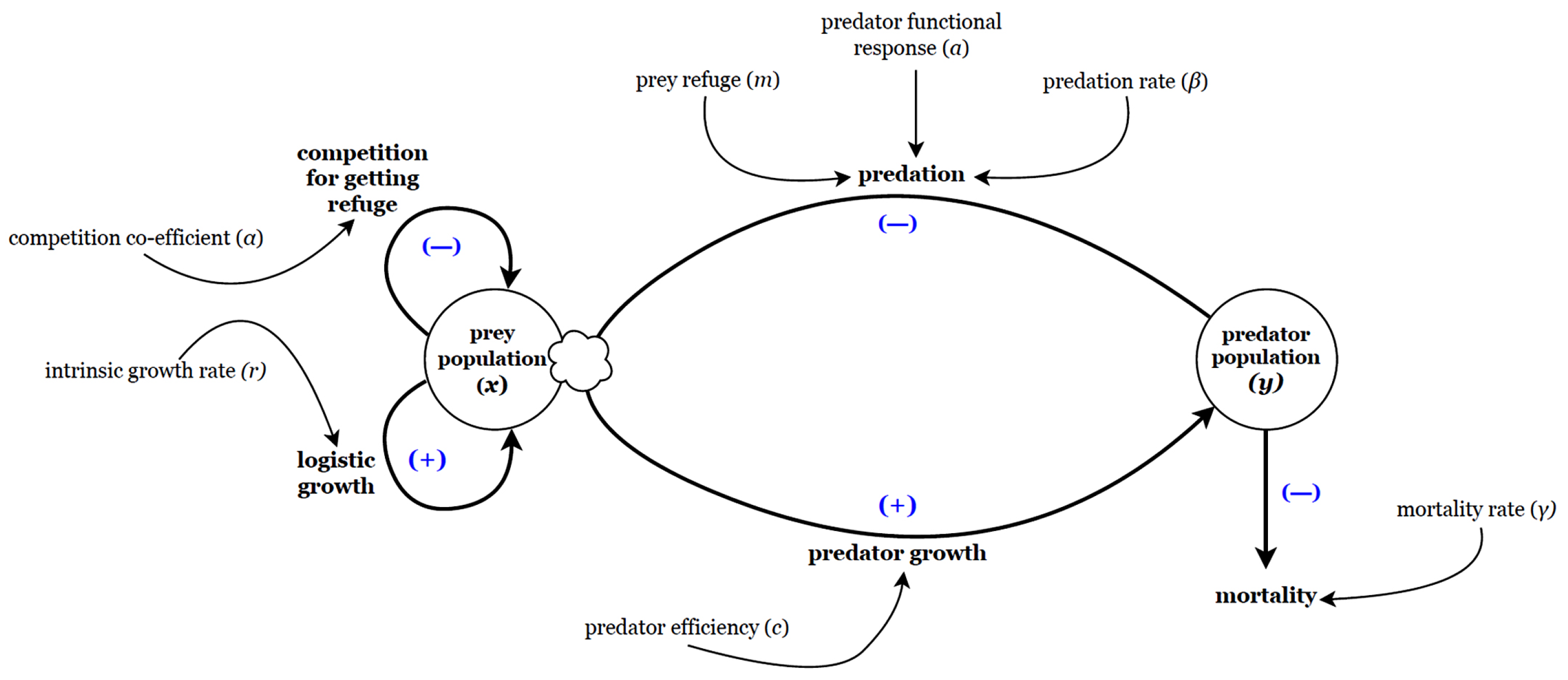
There are two populations in the model. $x\left(t\right)$ is the prey population size and $y\left(t\right)$ is the population size of the predator at any time t. r is the intrinsic growth rate, and k is the carrying capacity of the prey. $\gamma$ is the death rate of the predator in the absence of prey, $\beta$ is the predation rate, and c is the conversion factor that denotes the efficiency of predators for each captured prey.

Also, $\frac{\beta }{a}$ is the maximum number of prey that the predator can eat per unit time; $\frac{1}{a}$ is the half-saturation constant.

The term $\frac{\beta x}{1+ax}$ denotes the predator’s response to prey. This type of predator response function is known as a Holling type II functional response.

Let m be the fractional refuge of prey from the predators, where $0<m<1$ and is constant. So, the $mx\left(t\right)$ portion of the prey is in the refuge habitat, and the $(1-m)x\left(t\right)$ portion of the prey is in open habitats and is thus available to the predator, and $\theta$ is the cooperation coefficient among the prey population trying to escape predation pressure through refuge.

Using the assumptions discussed above, we obtain the following mathematical model:

$$\begin{array}{ccc}\hfill \frac{dx}{dt}& =& rx\left[1-\frac{x}{k}\right]-\frac{\beta (1-m)xy}{1+a(1-m)x}+\theta x^2,\hfill \\ \hfill \frac{dy}{dt}& =& -\gamma y+\frac{c\beta (1-m)xy}{1+a(1-m)x},\hfill \end{array}$$

(1)

with the initial biological condition

$$x\left(0\right)>0,y\left(0\right)>0$$

(2)

It is assumed that all system parameters are positive constants. A schematic diagram of the model (1) is shown in Figure 1.

In the next subsection, we determine all the possible equilibrium points and existence conditions for the biological feasibility of the model (1).

2.1. Boundedness of Solutions

Biologically, all populations in the model should be finite. For this, a boundedness analysis is significant. We derived the following theorem for the boundedness of the solutions to the model (1).

Theorem 1. 

All solutions to the model (1) with the given initial conditions (2) are non-negative and bounded for all time periods $t>0$.

Proof. 

We rewrite the first equation of (1),

$$\begin{array}{ccc}\hfill \frac{dx}{dt}& =& rx\left[1-\frac{x}{k}\right]-\frac{\beta (1-m)xy}{1+a(1-m)x}+\theta x^2=xh(x,y),\hfill \end{array}$$

(3)

where $h(x,y)=r\left[1-\frac{x}{k}\right]-\frac{\beta (1-m)y}{1+a(1-m)x}+\theta x$. Therefore,

$$\begin{array}{ccc}\hfill \frac{dx}{x}& =& h(x,y)dt\hfill \\ \hfill x\left(t\right)& =& x\left(0\right)exp\left\{{\int }_0^{t}h(x,y)dt\right\}\hfill \end{array}$$

Since $x\left(0\right)>0$, we can conclude that $x\left(t\right)$ is always positive. Similarly, the non-negativity of $y\left(t\right)$ can be established.

For the boundedness analysis, we define $W=x+y$. Now, adding the two equations of (1), we can obtain

$$\begin{array}{ccc}\hfill \frac{dW}{dt}& =& rx\left[1-\frac{x}{k}\right]-\frac{\beta (1-m)xy}{1+a(1-m)x}+\theta x^2-\gamma y+\frac{c\beta (1-m)xy}{1+a(1-m)x},\hfill \end{array}$$

By definition, $c\le 1$. Using this fact, we can write

$$\begin{array}{ccc}\hfill \frac{dW}{dt}& \le & rx\left[1-\frac{x}{k}\right]+\theta x^2-\gamma y\hfill \\ & =& rx\left[1-\frac{x}{k}\right]+\theta x^2-\gamma (x+y)+\gamma x.\hfill \end{array}$$

(4)

Now, $g\left(x\right)=rx\left[1-\frac{x}{k}\right]+\theta x^2+\gamma x$ is a function of x only. It has a maximum value at $x=\frac{k(r+\gamma )}{2(r-k\theta )}$, and the maximum value is $M_{\theta }=\frac{k{(r+\gamma )}^2}{4(r-k\theta )}$. Thus, from (4), we obtain

$$\begin{array}{ccc}\hfill \frac{dW}{dt}& \le & M_{\theta }-\gamma W\hfill \end{array}$$

Using the theory of functional differential equation, we have

$$lim\underset{t\to \infty }{sup}W=\frac{M_{\theta }}{\gamma }.$$

(5)

□

The set $\mathcal{D}$ is defined by

$$\mathcal{D}=\{(x,y)\in {\mathbb{R}}_{+}^2:0\le x+y\le M_{\theta },r>k\theta \}$$

(6)

where $M_{\theta }=\frac{k{(r+\gamma )}^2}{4(r-k\theta )}$, is positively invariant and each solution that starts in $\mathcal{D}$ remains in $\mathcal{D}$.

2.2. Existence of Equilibria

In this subsection, we analyze the existence and stability of the positive solution to the system (1).

Model (1) has three equilibrium points, viz., (i) the trivial equilibrium ${\overline{E}}_0(0,0)$, (ii) the predator-free equilibrium ${\overline{E}}_1\left(\frac{rk}{r-\theta k},0\right)$, and (iii) the coexisting equilibrium ${\overline{E}}^{*}({\overline{x}}^{*},{\overline{y}}^{*})$, where

$$\begin{array}{c}\hfill {\overline{x}}^{*}=\frac{\gamma }{(1-m)(c\beta -a\gamma )},\\ \hfill {\overline{y}}^{*}=\frac{1}{\beta (1-m)}\{1+a(1-m){\overline{x}}^{*}\}\left[\theta {\overline{x}}^{*}+\frac{r(k-{\overline{x}}^{*})}{k}\right].\end{array}$$

(7)

Now $y^{*}$ is positive if $\theta {\overline{x}}^{*}+\frac{r(k-{\overline{x}}^{*})}{k}>0$ which, after simple calculations, gives ${\overline{x}}^{*}>\frac{rk}{r-\theta k}$.

Using the fact that $0<m<1$ and from the above discussion, we have the following result for the existence of the equilibria of the system (1).

Proposition 1. 

(i) 

The predator-free equilibrium of the system (1) is feasible if $\theta <\frac{r}{k}$, and

(ii) 

the coexisting equilibrium ${\overline{E}}^{*}$ is feasible if $\frac{c\beta }{a}>\gamma$ and ${\overline{x}}^{*}>\frac{rk}{r-\theta k}$.

Remark 1. 

When the cooperation for attaining refuge (θ) is less than the overall intra-specific competition in the logistic growth of prey ($\frac{r}{k}$), the predator-free equilibrium ${\overline{E}}_1$ of the system (1) is feasible; otherwise, it will not exist. On the other hand, when the utilization efficiency of predators after successful predation ($\frac{c\beta }{a}$) is greater than the mortality rate of predators in the absence of prey (γ), then the coexisting equilibrium ${\overline{E}}^{*}$ will exist.

2.3. Stability Analysis and Hopf Bifurcation

Here, we examine the stability of each biologically feasible equilibrium. We perturb the ODE system near to any equilibrium point $\overline{E}(x,y)$ and obtain the system

$$\frac{dX}{dt}=JX,$$

where $X={[x,y]}^T$ and J is the Jacobian matrix.

The Jacobian J for the system (1) is

$$J=\left[J_{ij}\right]=\left[\begin{array}{cc}rx(1-\frac{2x}{k})-\frac{\beta (1-m)y}{{(1+a(1-m)x)}^2}+2\theta x& -\frac{\beta (1-m)x}{1+a(1-m)x}\\ \\ \frac{c\beta (1-m)y}{{(1+a(1-m)x)}^2}& -\gamma +\frac{c\beta (1-m)x}{(1+a(1-m\left)x\right)}\end{array}\right].$$

A characteristic equation of the Jacobian matrix is given by

$$f\left(\xi \right)={\xi }^2+l_1\xi +l_2=0.$$

(8)

An equilibrium point $E(x,y)$ is stable if both the roots of (8) are negative or have negative real parts. The conditions for this are

$$l_1>0\mathrm{and}{l}_2>0,$$

(9)

where

$$l_1=-(J_{11}+J_{22}),l_2=J_{11}{J}_{22}-J_{21}{J}_{12}.$$

The equilibrium $E(x,y)$ is unstable if any of the above conditions are violated.

Hopf bifurcation will occur if both the roots of (8) are purely imaginary for a particular value of the model parameter (called the bifurcation parameter). Suppose $\eta$ is a bifurcation parameter. Then, for bifurcation to occur, the following condition must be satisfied:

$$\begin{array}{ccc}& \left(i\right)& l_1=0,l_2>0,\hfill \\ \hfill & \left(ii\right)& \frac{\partial l_1}{\partial \eta }\ne 0.\hfill \end{array}$$

(10)

Condition (i) will give the critical value of the bifurcation parameter, and condition (ii) is the transversality condition.

The Jacobian matrix J at the trivial equilibrium ${\overline{E}}_0(0,0)$ has a positive eigenvalue r; thus, it is always unstable.

At the predator-free equilibrium ${\overline{E}}_1(\overline{x_1},0)$, the Jacobian matrix is

$$J\left({\overline{E}}_1\right)=\left[\begin{array}{cc}r\overline{x_1}(1-\frac{2\overline{x_1}}{k})+2\theta \overline{x_1}& -\frac{\beta (1-m)\overline{x_1}}{1+a(1-m)\overline{x_1}}\\ 0& -\gamma +\frac{c\beta (1-m)\overline{x_1}}{(1+a(1-m)\overline{x_1})}\end{array}\right],$$

where $\overline{x_1}=\frac{rk}{r-\theta k}$.

${\overline{E}}_1$ is always feasible as $\frac{r}{k}>\theta$ is true for the model (1). The Jacobian matrix has eigenvalues ${\xi }_1=r\overline{x}(1-\frac{2\overline{x}}{k})+2\theta \overline{x}$ and is negative for $\frac{r}{k}>\theta$, directly following on from the feasibility of ${\overline{E}}_1$. Another eigenvalue is ${\xi }_2=-\gamma +\frac{c\beta (1-m)\overline{x}}{(1+a(1-m)\overline{x})}$, which is negative if $\theta >\frac{r\gamma -rk\left[c\beta \right(1-m)-a(1-m\left)\gamma \right]}{\gamma k}$.

The characteristic equation at the coexisting equilibrium ${\overline{E}}^{*}$ is

$${\xi }^2+{\overline{l}}_1^{*}\xi +{\overline{l}}_2^{*}=0,$$

(11)

where

$${\overline{l}}_1^{*}=-r{\overline{x}}^{*}(1-\frac{2{\overline{x}}^{*}}{k})+\frac{\beta (1-m){\overline{y}}^{*}}{{(1+a(1-m){\overline{x}}^{*})}^2}-2\theta {\overline{x}}^{*},$$

$${\overline{l}}_2^{*}=\frac{c{\beta }^2{(1-m)}^2{\overline{x}}^{*}{\overline{y}}^{*}}{{(1+a(1-m){\overline{x}}^{*})}^3}>0.$$

The eigenvalues are negative or have negative real parts if ${\overline{l}}_1^{*}>0$ as ${\overline{l}}_2^{*}>0$ always holds.

From the above discussion, we have the following theorem for the stability of the three equilibriums of system (1).

Theorem 2. 

(i) 

The trivial equilibrium ${\overline{E}}_0(0,0)$ is always unstable.

(ii) 

${\overline{E}}_1$ is always feasible and is stable if $\theta <\frac{r\gamma -rk(1-m)[c\beta -a\gamma ]}{\gamma k}$; consequently, transcritical bifurcation occurs if $\theta =\frac{r\gamma -rk(1-m)[c\beta -a\gamma ]}{\gamma k}$.

(iii) 

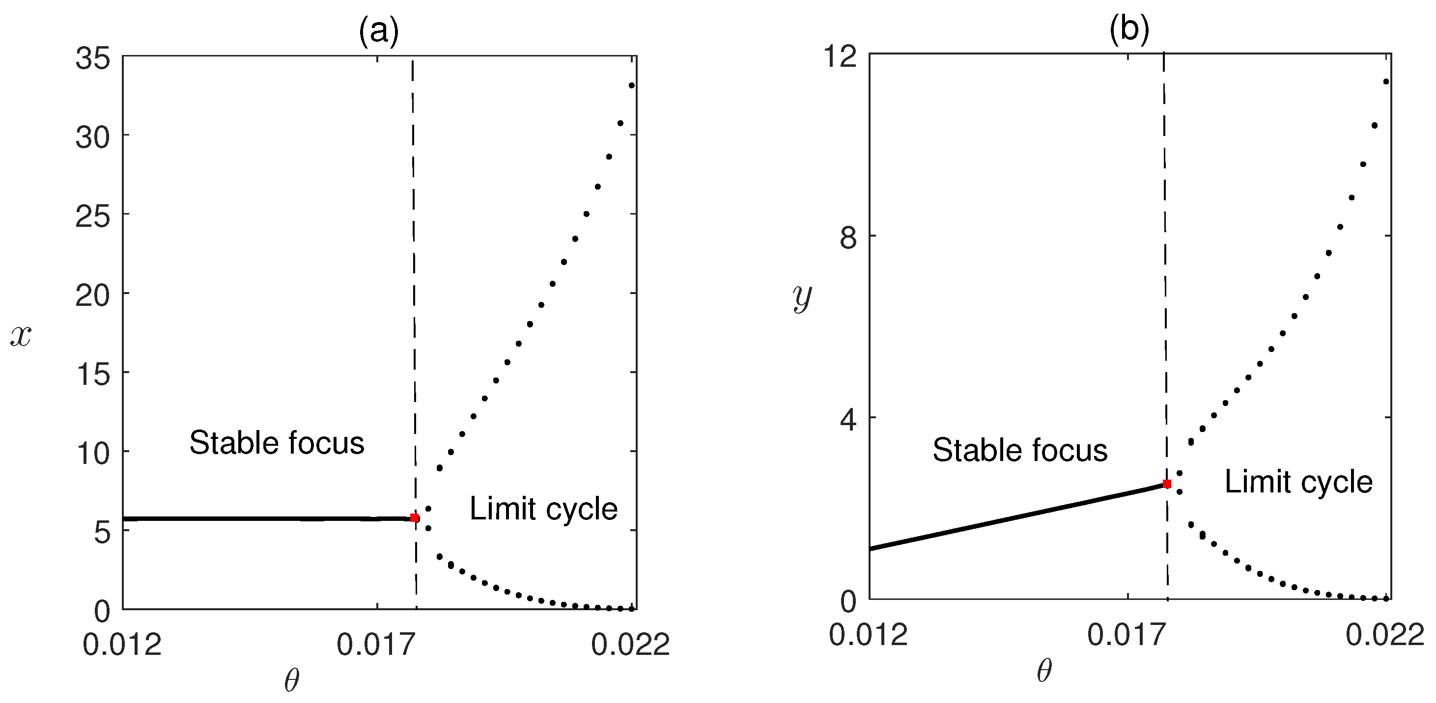
${\overline{E}}^{*}$ is stable if ${\overline{l}}_1^{*}>0$ and unstable for ${\overline{l}}_1^{*}<0$. Hopf bifurcation occurs if ${\overline{l}}_1^{*}=0$ and $\frac{\partial l_1^{*}}{\partial \theta }{|}_{\theta ={\theta }^{*}}\ne 0$, where ${\theta }^{*}$ is the critical value of the bifurcation parameter θ.

2.4. Global Stability of $E^{*}$

The following theorem establishes the global stability of the interior equilibrium $E^{*}$.

Theorem 3. 

The interior equilibrium $E^{*}$ is globally asymptotically stable if the conditions mentioned below are satisfied:

$$\begin{array}{ccc}\hfill & \left(i\right)& k\theta <r,\hfill \\ & \left(ii\right)& \frac{rk}{\theta k-r}<x^{*}<\frac{\gamma }{\beta }.\hfill \end{array}$$

(12)

Proof. 

We construct the suitable Lyapunov function V as

$$V=(x-x^{*}-x^{*}ln\frac{x}{x^{*}})+(y-y^{*}-y^{*}ln\frac{y}{y^{*}}).$$

(13)

It is easy to verify that V is positive definite for all $(x,y)\in R_{+}^2\setminus (x^{*},y^{*})$. Now, we take the derivative of V along the solutions of the system (1) and obtain the following:

$$\begin{array}{ccc}\hfill \frac{dV}{dt}& =& (x-x^{*})\frac{\dot{x}}{x}+(y-y^{*})\frac{\dot{y}}{y},\hfill \\ & =& (x-x^{*})\left[r\left[1-\frac{x}{k}\right]-\frac{\beta (1-m)y}{1+a(1-m)x}+\theta x\right]+(y-y^{*})\left[-\gamma +\frac{c\beta (1-m)x}{1+a(1-m)x}\right].\hfill \end{array}$$

By rearranging equation (14) we obtain the following:

$$\begin{array}{ccc}\hfill \frac{dV}{dt}& =& x^2(-\frac{r}{k}+\theta )+x(r+\frac{r{x}^{*}}{k}-\theta x^{*})-r{x}^{*}+\left(\frac{c\beta xy}{1+ax}-\frac{\beta xy}{1+ax}\right)+\left(\frac{\beta x^{*}y}{1+ax}-\gamma y\right)\hfill \\ & & -\frac{c\beta x{y}^{*}}{1+ax}-\gamma y^{*}-\gamma y+y\left(\frac{\beta x^{*}}{1+ax}-\gamma \right).\hfill \end{array}$$

Thus, if the conditions given in (12) hold, then the right-hand side of (14) is negative definite. Thus, $\frac{dV}{dt}<0$ along all trajectories in the first quadrant except $(x^{*},y^{*})$. Also, we have $\frac{dV}{dt}{|}_{E^{*}}=0$. The proof follows on from the suitable Lyapunov function V and Lyapunov–LaSalle’s invariant principle (cf. Hale [36]). Hence, the interior equilibrium point $E^{*}$ is globally asymptotically stable if condition (12) is satisfied. □

3. The Mathematical Model for Prey Refuge and Intra-Specific Competition

The flow chart of this situation is given in Figure 2. From this, we propose the Lotka–Volterra type prey–predator system, including the proportional prey refuge and competition, as follows:

$$\begin{array}{ccc}\hfill \frac{dx}{dt}& =& rx\left[1-\frac{x}{k}\right]-\frac{\beta (1-m)xy}{1+a(1-m)x}-\alpha x^2,\hfill \\ \hfill \frac{dy}{dt}& =& -\gamma y+\frac{c\beta (1-m)xy}{1+a(1-m)x}.\hfill \end{array}$$

(14)

where $\alpha$ is the competition coefficient among the prey population trying to escape predation pressure through refuge, and all other parameters were already defined in the previous model (1).

Remark 2. 

From a mathematical point of view, model (1) and model (14) differ only in one term: $-\alpha x^2$ in place of $\theta x^2$. Thus, the analytical results (dynamics) of model (14) can be derived from the analysis of model (1).

From the analysis presented in the previous section (using Theorem 1) we derived the following theorem.

3.1. Boundedness of Solutions

Theorem 4. 

Each solution to model (14) with positive initial conditions remains non-negative and bounded in $\mathcal{S}$ for all time points $t>0$, where

$$\mathcal{S}=\{(x,y)\in {\mathbb{R}}_{+}^2:0\le x+y\le M_{\alpha },\}$$

(15)

where $M_{\alpha }=\frac{k{(r+\gamma )}^2}{4(r+k\alpha )}.$

3.2. Existence of Equilibria

Model (14) has three equilibrium points, viz., (i) the trivial equilibrium ${\tilde{E}}_0(0,0)$, (ii) the predator-free equilibrium ${\tilde{E}}_1(\frac{rk}{r+\alpha k},0)$, and (iii) the coexisting equilibrium ${\tilde{E}}^{*}({\tilde{x}}^{*},{\tilde{y}}^{*})$, where

$$\begin{array}{ccc}\hfill {\tilde{x}}^{*}& =& \frac{\gamma }{(1-m)(c\beta -a\gamma )},\hfill \end{array}$$

(16)

$$\begin{array}{ccc}\hfill {\tilde{y}}^{*}& =& \frac{1}{\beta (1-m)}\{1+a(1-m){\tilde{x}}^{*}\}\left[-\alpha {\tilde{x}}^{*}+\frac{r(k-{\tilde{x}}^{*})}{k}\right].\hfill \end{array}$$

(17)

In model (14), ${\tilde{E}}_1$ always exists, and ${\tilde{E}}^{*}$ exists for $\frac{c\beta }{a}>\gamma$ and $-\alpha {\tilde{x}}^{*}+\frac{r(k-{\tilde{x}}^{*})}{k}>0$. The last condition gives ${\tilde{x}}^{*}<\frac{rk}{k\alpha +r}$. Thus, we have the following result.

Proposition 2. 

(i) 

The predator-free equilibrium of the system (14) always exists.

(ii) 

The coexisting equilibrium ${\tilde{E}}^{*}$ is feasible if $\frac{c\beta }{a}>\gamma$ and ${\tilde{x}}^{*}<\frac{rk}{r+\alpha k}$.

Remark 3. 

In model (1), the existence of the predator-free equilibrium ${\overline{E}}_1$ depends on θ, but in model (14), the equilibrium always exists. One major explanation for the cooperation for attaining refuge (θ) may cause behavioral contradictions among the prey population as they compete in almost all aspects, except finding refuge, and for that reason, θ becomes a critical factor for the existence of the equilibrium.

3.3. Stability and Hopf Bifurcation

The Jacobian at any steady point $\tilde{E}(x,y)$ of system (14) is given below:

$$J\left(E\right)=\left[J_{ij}\right]=\left[\begin{array}{cc}rx(1-\frac{2x}{k})-\frac{\beta y}{{(1+ax)}^2}-2\alpha x& -\frac{\beta x}{1+ax}\\ \\ \frac{c\beta y}{{(1+ax)}^2}& -\gamma +\frac{c\beta x}{(1+ax)}\end{array}\right].$$

Using the stability analysis of the previous section (using Theorem 2, we can establish the following theorem for the stability of the equilibrium points in the system (14).

Theorem 5. 

(i) 

The trivial equilibrium ${\tilde{E}}_0(0,0)$ is always unstable.

(ii) 

${\tilde{E}}_1$ is stable if $\alpha <\frac{rk(1-m)[c\beta -a\gamma ]-r\gamma }{\gamma k}$ and unstable for $\alpha >\frac{rk(1-m)[c\beta -a\gamma ]-r\gamma }{\gamma k}$. Consequently, transcritical bifurcation occurs at $\alpha =\frac{rk(1-m)[c\beta -a\gamma ]-r\gamma }{\gamma k}$.

(iii) 

${\tilde{E}}^{*}$ is stable if ${\tilde{l}}_1^{*}>0$ and unstable for ${\tilde{l}}_1^{*}<0$. Hopf bifurcation occurs if ${\tilde{l}}_1^{*}=0$ and $\frac{\partial {\tilde{l}}_1^{*}}{\partial \alpha }{|}_{\alpha ={\alpha }^{*}}\ne 0$, where ${\alpha }^{*}$ denotes the critical value of the bifurcation parameter α. In this case,

$${\tilde{l}}_1^{*}=-r{\tilde{x}}^{*}(1-\frac{2{\tilde{x}}^{*}}{k})+\frac{\beta (1-m){\tilde{y}}^{*}}{{(1+a(1-m){\tilde{x}}^{*})}^2}+2\alpha {\tilde{x}}^{*},$$

and

$${\tilde{l}}_2^{*}=\frac{c{\beta }^2{(1-m)}^2{\tilde{x}}^{*}{\tilde{y}}^{*}}{{(1+a(1-m){\tilde{x}}^{*})}^3}>0.$$

3.4. Direction of Hopf Bifurcation

In this section, we analyze the stability nature and direction of the Hopf bifurcating periodic solutions. For this, we consider the transformation, $u_1=x-x_{*}$, $u_2=y-y_{*}$, which transform the system (1) into the following system,

$$\begin{array}{ccc}\hfill {\dot{u}}_1& =& a_1{u}_1+a_2{u}_2+\underset{i,j\ge 0}{\sum _{i+j=2}}{a}_{ij}{u}_1^i{u}_2^j+\underset{i,j\ge 0}{\sum _{i+j=2}}{a}_{ij}{u}_1^i{u}_2^j+\cdots \hfill \end{array}$$

(18)

$$\begin{array}{ccc}\hfill {\dot{u}}_2& =& b_1{u}_1+b_2{u}_2+\underset{i,j\ge 0}{\sum _{i+j=2}}{b}_{ij}{u}_1^i{u}_2^j+\underset{i,j\ge 0}{\sum _{i+j=2}}{b}_{ij}{u}_1^i{u}_2^j+\cdots ,\hfill \end{array}$$

(19)

where $a_{ij}$ and $b_{ij}$ are determined by using the following relations:

$$\begin{array}{c}\hfill a_{ij}=\frac{1}{i!j!}\frac{{\partial }^{i+j}\left(F_1\right)}{\partial x^i\partial y^j},b_{ij}=\frac{1}{i!j!}\frac{{\partial }^{i+j}\left(F_2\right)}{\partial y^i\partial y^j}.\end{array}$$

(20)

where $a_1=\frac{\partial F_1}{\partial x}$, $a_2=\frac{\partial F_2}{\partial y}$, etc., and

$$\begin{array}{c}\hfill F_1=rx\left[1-\frac{x}{k}\right]-\frac{\beta (1-m)xy}{1+a(1-m)x}-\alpha x^2,\\ \hfill F_2=-\gamma y+\frac{c\beta (1-m)xy}{1+a(1-m)x}.\end{array}$$

We obtain the following relations from Hassard et al. [37],

$$\begin{array}{c}\hfill \left[\begin{array}{c}{u}_1\\ u_2\end{array}\right]=zq+\overline{z}\overline{q}+W,\end{array}$$

(21)

where

$$\begin{array}{c}\hfill z\left(t\right)=\langle q^{*},u_t\rangle ,W(t,\theta )=u_t\left(\theta \right)-2\mathrm{Re}\left\{z\left(t\right)q\left(\theta \right)\right\}.\end{array}$$

(22)

Thus,

$$\begin{array}{ccc}\hfill \dot{z}& =& i{\omega }_{0}z+{\overline{v}}_1{f}_0^1+{\overline{v}}_2{f}_0^2+{\overline{v}}_3{f}_0^3\hfill \\ & =& i{\omega }_{0}z+\frac{1}{2}{g}_{20}{z}^2+g_{11}z\overline{z}+\frac{1}{2}{g}_{02}{\overline{z}}^2+\frac{1}{6}{g}_{30}{z}^3+\frac{1}{6}{g}_{03}{\overline{z}}^3+\frac{1}{2}{g}_{21}{z}^2\overline{z}+\frac{1}{2}{g}_{12}z{\overline{z}}^2\hfill \\ & +& \mathrm{O}\left(\right|z{|}^4),\hfill \end{array}$$

(23)

We calculate the values of $g_{20}$, $g_{02}$, $g_{11}$ and $g_{21}$ by comparing the coefficients of $z^2$, ${\overline{z}}^2$, $z\overline{z}$ and $z^2\overline{z}$. Hence,

$$\begin{array}{ccc}\hfill C_1\left(0\right)& =& \frac{i}{2{\omega }_0}\left(g_{11}{g}_{20}-2{\left|g_{11}\right|}^2-\frac{|g_{02}{|}^2}{3}\right)+\frac{g_{21}}{2},\hfill \end{array}$$

(24a)

$$\begin{array}{ccc}\hfill {\mu }_2& =& -\frac{\mathrm{Re}\left(C_1\left(0\right)\right)}{\mathrm{Re}\left({\eta }^{\prime }\left(0\right)\right)},\hfill \end{array}$$

(24b)

$$\begin{array}{ccc}\hfill {\beta }_2& =& 2\mathrm{Re}\left(C_1\left(0\right)\right),\hfill \end{array}$$

(24c)

$$\begin{array}{ccc}\hfill {\tau }_2& =& -\frac{\mathrm{Im}\left(C_1\left(0\right)\right)+{\mu }_2\mathrm{Im}\left({\eta }^{\prime }\left(0\right)\right)}{{\omega }_0},\hfill \end{array}$$

(24d)

where

$$\begin{array}{c}\hfill \mathrm{Im}\left({\eta }^{\prime }\left(0\right)\right)=\frac{\mathrm{d}\left(\mathrm{Im}\left(\eta \right(\alpha \left)\right)\right)}{\mathrm{d}\alpha }{\mid }_{\alpha ={\alpha }^{*}}=\left[\frac{{\sigma }_1}{\sqrt{{\sigma }_2}}\frac{\dot{{\sigma }_3}-(\dot{{\sigma }_1}{\sigma }_2+{\sigma }_1\dot{{\sigma }_2})}{2({\sigma }_1^2+{\sigma }_2)}+\frac{({\sigma }_1+{\sigma }_2){\dot{\sigma }}_2}{2\sqrt{{\sigma }_2}({\sigma }_1^2+{\sigma }_2)}\right]{\mid }_{\alpha ={\alpha }^{*}}.\end{array}$$

The stability and direction can be determined from the following theorem [29,38].

Theorem 6. 

The nature of the bifurcating periodic solutions can be determined from the values of ${\beta }_2,{\mu }_2$, and ${\tau }_2$ in the center manifold at the threshold value ${\alpha }^{*}$.

(i) 

If ${\mu }_2$ is positive (negative), then the system (1) emits a stable (unstable) limit cycle for $\alpha >{\alpha }^{*}$ ($\alpha <{\alpha }^{*}$);

(ii) 

${\beta }_2$ determines the stability of the bifurcating periodic solutions, where the bifurcating periodic solutions are stable (unstable) if ${\beta }_2<0$$({\beta }_2>0)$; and

(iii) 

${\tau }_2$ determines the period of periodic solutions:, where the period increases (decreases) if ${\tau }_2>0$$({\tau }_2<0)$.

Remark 4. 

A similar theorem can be obtained for the parameter θ from Theorem 6.

4. Numerical Simulations

In this section, we provide numerical examples for visualizing the dynamical regimes that can be seen in our model systems analyzed in the previous sections. Parameter values with detailed descriptions and the units used for the simulation are given in

Table 1. List of parameters used in numerical simulations and their references.

Parameter	Definition	Value (Units)	References
r	intrinsic growth rate	0.1 prey${}^{-1}$ day${}^{-1}$	[34]
k	carrying capacity of the prey	4  individuals	[34]
$\beta$	predation rate	0.3 predator${}^{-1}$ day${}^{-1}$	[29]
c	conversion efficiency	$0<c<1$, predator prey${}^{-1}$	[29]
a	half-saturation constant	0.5, prey${}^{-1}$	[34]
m	prey refuge	$0\le m<1$, [no unit]	standard range
$\gamma$	death rate of predators	0.1 predator${}^{-1}$ day${}^{-1}$	[34]
$\theta$	cooperation coefficient among prey	$0\le \theta <1$ prey${}^{-1}$ day${}^{-1}$	standard range
$\alpha$	competition coefficient among prey	$0\le \alpha <1$ prey${}^{-1}$ day${}^{-1}$	standard range

. The value of the carrying capacity is taken as $k=4$, assuming that the maximum number of four prey can be supported within a 3 m × 3 m square area. Although the conversion efficiency (c) varies within a range of 0–1, we considered $c=0.75$ for the simulations. The results obtained from simulations, using the ode45 solver in Matlab are discussed in the following subsections.

4.1. Numerical Simulation of System (1)

In this subsection, a simulation of the system (1) is presented in Figure 3, Figure 4, Figure 5, Figure 6, Figure 7 and Figure 8 based on the calculations made in Section 2. In Figure 3, we plot the transcritical forward bifurcation between ${\overline{E}}_1$ and $E^{*}$ by varying the parameter $\theta$. For some large values of $\theta$, ${\overline{E}}^{*}$ becomes feasible (according to Theorem 2).

In Figure 4, we can see the limit cycle for $m=0$ (other parameters are given in Table 1), i.e., the limit cycle can occur if refuge is neglected. But, if we take $m=0.3$ (i.e., $30\%$ of the total prey population is in the refuge habitat and the other $70\%$ is vulnerable to predation), the limit cycle disappears, and the coexisting equilibrium $E^{*}$ becomes a stable focus.

In Figure 5, we use $m=0.3$ and $\theta =0$ (i.e., there is no cooperation among the prey population for finding a refuge habitat), and the system is stable. Then, we increase the value of $\theta$ (i.e., increase cooperation among the prey individuals for finding a safe refuge place) and set the limit cycle to $\theta =0.005$ (other parameters are given in Table 1). From this, we can conclude that the impact of $\theta$ is destabilization of the stable, steady state.

Figure 6 plots three different initial values of the model variables. This shows the nonlinear stability of the coexisting equilibrium $E^{*}$. In Figure 7, we plot the Hopf bifurcation diagram, taking $\theta$ as the main parameter. A stable limit cycle appears, as the parameter $\theta$ crosses the critical value (Theorem 2).

In Figure 8, we plot the stable regions of the coexisting equilibrium in the $\theta$–$\beta$ and $\theta$–m parameter planes. Figure 8a shows how parameters $\theta$ and $\beta$ critically affect the stability of the system. We can observe that for the very low value of $\theta$, ${\overline{E}}^{*}$ is not feasible but ${\overline{E}}_1$ is stable, and as $\theta$ crosses its critical value, ${\overline{E}}^{*}$ becomes stable and the stability of ${\overline{E}}^{*}$ depends on the combined value of $\theta$ and $\beta$, as higher values can make the stable system unstable via Hopf bifurcation. In Figure 8b, a direct relationship between the parameters $\theta$ and m and the stability of the system is shown, where with an increased value of $\theta$, only a very high value of m can make the system stable.

From the simulations, we observe that $\theta$ is one of the critical parameters for the model’s system (1), and the stability of different equilibria depends on it. For very low values of $\theta$, ${\overline{E}}^{*}$ is not feasible, but ${\overline{E}}_1$ is stable, and as $\theta$ crosses its critical value, ${\overline{E}}^{*}$ becomes stable via transcritical bifurcation, and finally, further higher values can make ${\overline{E}}^{*}$ unstable via Hopf bifurcation (Theorem 2).

4.2. Numerical Simulation of System (14)

Simulations are presented for the dynamics of the system (14) in Figure 9, Figure 10, Figure 11, Figure 12 and Figure 13 based on the analytical analysis presented in Section 3.

In Figure 9, we plot the transcritical forward bifurcation of ${\tilde{E}}_1$ and the existence of ${\tilde{E}}^{*}$ with variations in the parameter $\alpha$ (Theorem 5, (ii)). A Hopf bifurcation diagram is plotted in Figure 10, taking $\alpha$ as the main parameter (using (Theorem 5 (iii)). The limit cycle disappears as the parameter $\alpha$ crosses the critical value ${\alpha }^{*}$.

In Figure 12, we show $m=0.3$, $\alpha =0.001$ (i.e., there is very little competition among the prey individuals for finding a refuge habitat), and the system is stable. Now, if we increase the value of $\alpha$ to 0.01 (i.e., the prey individuals become ten times more competitive in the process of finding a safe refuge place), the system stabilizes faster (other parameters are given in Table 1). From this, we can conclude that $\alpha$ has a stabilizing effect on the system.

In Figure 13, we plot the stable regions of the coexisting equilibrium in the $\alpha$–$\beta$ and $\alpha$–m parameter planes. The area of the stable region increases as both m and $\alpha$ are increased. But, $\beta$ can make the stable system unstable via Hopf bifurcation (Theorem 5 (iii)). The critical value of $\beta$ i.e., ${\beta }^{*}$ depends on the other model parameters, such as $\alpha$. Here, we show that the critical value of $\beta$ significantly depends on $\alpha$. In (b), we use a higher value of $\beta$, and then we vary $\alpha$ and m. We observe that ${\tilde{E}}^{*}$ changes its stability level to become stable, except for at higher values of m and $\alpha$. The stable condition is only shown in $E_1$ for higher values of m and $\alpha$.

Figure 11 also plots two different initial values of the model variables. This figure shows that the bifurcating periodic solutions are stable and the Hopf bifurcation is of the supercritical type (Theorem 6).

From the numerical simulations, we observe that for model system (14), the stability of different equilibria depends on the parameter $\alpha$. Here, for very low values of $\alpha$, ${\tilde{E}}^{*}$ is unstable, and it becomes stable as $\alpha$ crosses the critical value via Hopf bifurcation, but for very high values of $\alpha$, ${\tilde{E}}^{*}$ is not feasible, whereas ${\tilde{E}}_1$ becomes stable via transcritical bifurcation (Theorem 5, (ii)).

5. Discussion and Conclusions

A prey–predator system including prey refuge has been a sought-after topic among ecological and mathematical modelers for almost the last five decades. Previous studies have assured that refuge has a stabilizing effect on prey–predator dynamics. Several models have already been established to represent various conditions and situations. Still, another finding is that if the refuge class or fraction becomes too large, the predator faces food scarcity. The system becomes destabilized due to the extinction of the predator. But, in any natural system, all members of a prey population cannot avoid predation at any given time; thus, continuous decision pressure works among them. The refuge among the prey population can happen in two ways, cooperatively or competitively, and these two inevitable intra-specific interactions must affect prey–predator dynamics. This study identified the impacts of cooperation and intra-specific competition among prey populations trying to escape predation through refuge on the stability of prey–predator dynamics.

The ecological motivation behind the formation of the mathematical models comes from the Hoogly–Matla estuarine mangrove ecosystem, where several islands are situated and are crisscrossed by numerous creeks that originate from the main rivers. These creeks have rich detritus loads which come from the adjacent mangrove litter. Therefore, these creeks support many detritivorous fishes, and one such fish was described by Sarwardi et al. [34]. In their study, Sarwardi et al. [34] described one important detritivorous fish from these creeks, namely Liza parsia, which lives in the creeks, and its predator Otolithoides pama visits the creeks during high tide only to capture food. The mangrove plants in this region extend from the supra-littoral zone to the lower-littoral zone up to the creek bed. During high tide, as the water level comes up, the lower parts of the plants submerge under the water and the bushy part of the submerged mangrove plants creates shelter for Liza parsia to avoid its predator. So, this spatial refuge is possible due to enhanced environmental heterogeneity in this ecosystem. In many cases, due to an inadequate refuge habitat, all individuals of the prey population can not escape predation. In this situation, the prey population finds refuge either through cooperation or competition and avoids predation pressure. The present study focuses on the effects of these two important intra-specific interactions on the dynamics of prey–predator interaction with the prey refuge.

In a basic predator–prey model, the population dynamics of the predators and prey are influenced by factors such as predation, reproduction, and competition for resources. However, if we introduce cooperation and competition among the prey species themselves, the model becomes more complex. For the two situations mentioned above, in this paper, we considered a prey–predator system incorporating a prey refuge and assumed that the predator response function ia Holling type II. Cooperation (model (1)) and intra-specific competition (model (14)) among the prey population for escaping predation pressure through refuge are incorporated into the system to find out the process (either cooperation or intra-specific competition) that leads the population towards better stabilization.

Firstly, the stabilizing effect of refuge on the system dynamics was shown (Figure 4). After the addition of refuge, the system dynamics settle from limit cycle behavior to a stable equilibrium. The refuge protects the prey population from predators, and it reduces predation pressure. Over-exploitation of the prey population by predators moves the prey population into a divergent oscillation state. But, this vulnerable state is transformed into a stable state with the help of the prey population’s refuge strategies. The stable state of the prey population also makes a stable predator population.

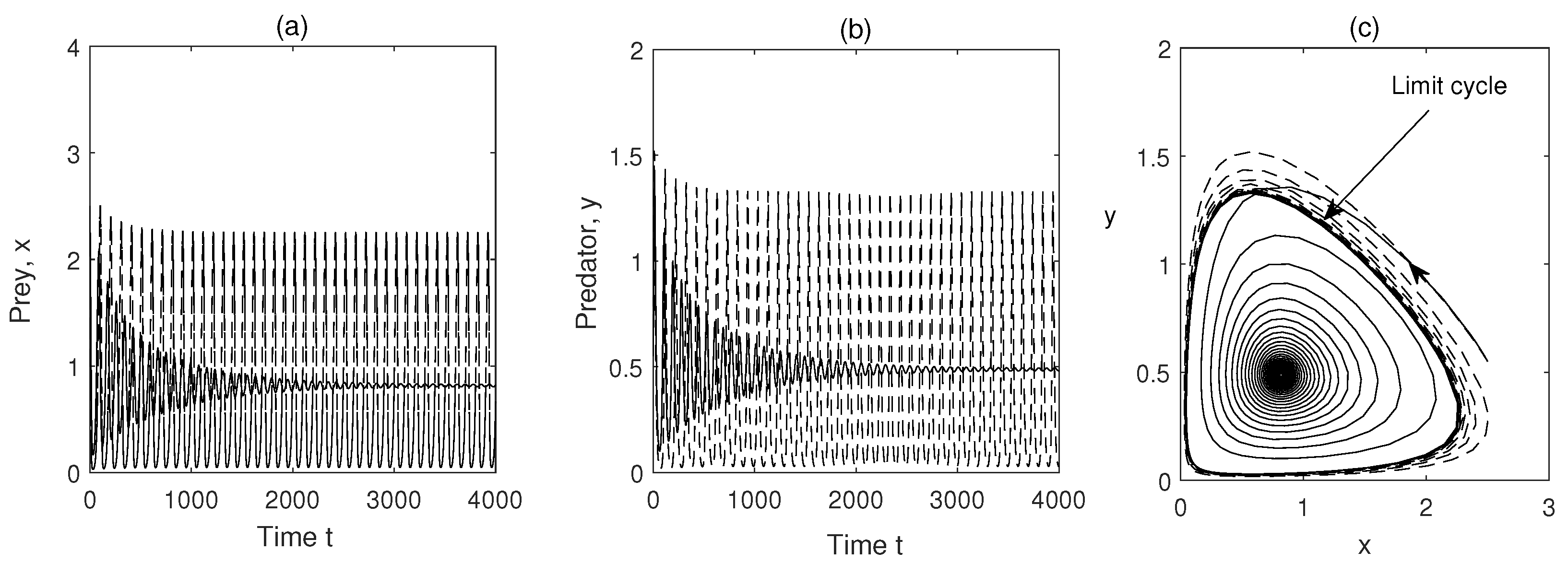
When the decision about refuge is made cooperatively among the prey population, the stable equilibrium again goes back to a limit cycle condition which clearly denotes that cooperation has a destabilizing effect on the system dynamics during refuge (Figure 5). From the prey’s point of view, if the refuge is attained cooperatively, then the maximum number of individuals can escape predator easily, which is favorable for them but on the other hand, predators will suffer from low predation success, and in an extreme situation, they will be eliminated from the system if the system is linear as a predator has no alternative option to predate.

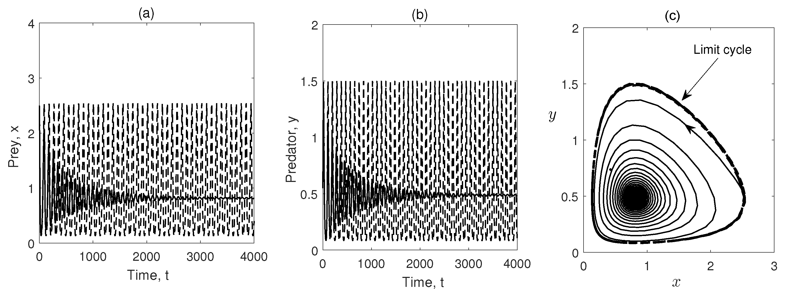
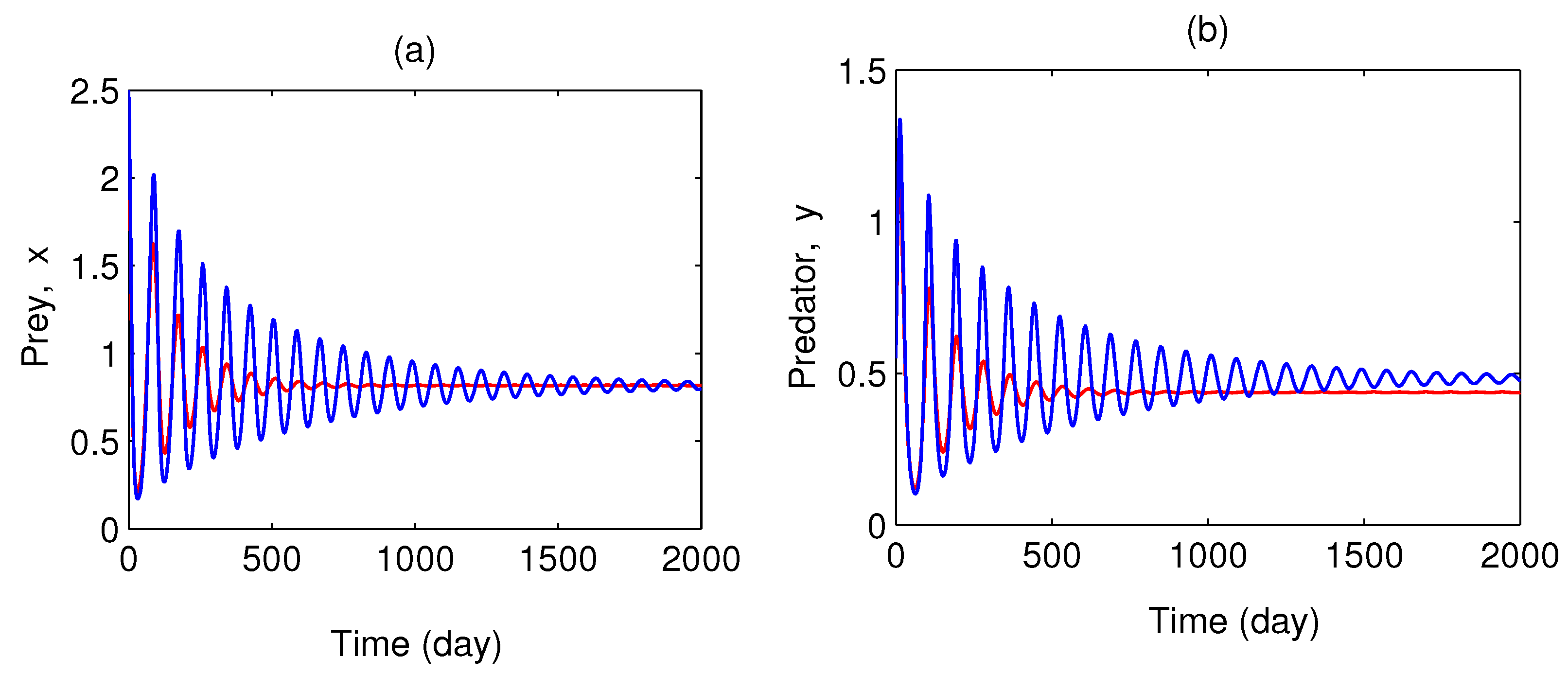
Our study shows that the system reaches the equilibrium state faster when the refuge facility is achieved through intra-specific competition among the prey population (Figure 12). Refuge during intra-specific competition has a stabilizing effect on the system dynamics. As intra-specific competition has a negative impact on individuals in the prey population, the refuge class is constantly controlled and never becomes too large to cause prey scarcity for a predator. A controlled amount of the prey population will always escape predators through refuge, which improves the survival of the prey population, and the predator population will not become extinct in any situation, as it never faces a food crisis. Due to this balanced interaction, the system dynamics reach an equilibrium faster.

In reality, the decision-making process to escape predation pressure by refuge either through competition or cooperation within a prey population is complex and does not follow any hard and fast rules. Cooperation or competition in various prey organisms depends on the spatial heterogeneity of the habitat, as when the shelter place (refuge size) is large enough to protect all prey individuals, only cooperation acts as the deciding factor, but any scarcity in the protected habitat turns the cooperative behavior into a competitive one.

It is more difficult for a prey population to escape predation through refuge individually than by living in a group and cooperating conspecifically. Group living in a prey population has many facilities from the perspective of refuge, as it reduces the chance of detection by the predator due to the presence of many eyes and ears that are attuned to predation threats [39,40]. So, cooperation plays a major role in attaining refuge within a living prey population group, but this is not necessarily always the case. Underlying intra-specific competition may be found among the group members, which can be explained by the selfish-herd effect [41,42]. Though each member enjoys the benefit of decreasing the domain of danger when living in a group than as a solitary forager, those individuals who are present outside the group still have a larger domain of danger compared to those at the core, and thus, they may compete with each other to take shelter at the core of the group [39,43]. This study fills the research gap by dealing with the impacts of cooperation and intra-specific competition among the prey population for escaping from predators through refuge on the prey–predator system, and it was found that when the prey individuals become competitive with each other for shelter in the refuge habitat, the system dynamics achieve stability faster. On the other hand, any cooperation among the prey population regarding refuge turns the stable equilibrium into a limit cycle condition.

Interactions in the living world are very complex, and it is difficult to conclude whether competition or cooperation is helpful for refuges. A high rate of parental care has been observed in many bird species, including the protection of offspring from predators by forming nests. In such cases, the parents cooperate with their offspring for successful refuge, but at the same time, the offspring may compete to achieve successful refuge. In reality, when prey populations are small, they need cooperation rather than competition, but the reverse situation is noticed in case of large prey populations. Therefore, both cooperation and competition are inevitable processes during the refuge of the prey population, and the selection of either cooperation or competition depends on the conditions within the prey population.