Article

A Quantile Functions-Based Investigation on the Characteristics of Southern African Solar Irradiation Data

1
Department of Statistics and Operations Research, University of Limpopo, Private Bag X1106, Sovenga 0727, South Africa
2
Department of Statistics and Operations Research, National University of Science and Technology, Ascot, Bulawayo P.O. Box AC 939, Zimbabwe
*
Author to whom correspondence should be addressed.
Math. Comput. Appl. 2023, 28(4), 86; https://doi.org/10.3390/mca28040086
Submission received: 19 May 2023 / Revised: 4 July 2023 / Accepted: 19 July 2023 / Published: 24 July 2023
(This article belongs to the Special Issue Statistical Inference in Linear Models)

Abstract

:
Exploration of solar irradiance can greatly assist in understanding how renewable energy can be better harnessed. It helps in establishing the solar irradiance climate in a particular region for effective and efficient harvesting of solar energy. Understanding the climate provides planners, designers and investors in the solar power generation sector with critical information. However, a detailed exploration of these climatic characteristics has not yet been studied for the Southern African data. Very little exploration is being done through the use of measures of centrality only. These descriptive statistics may be misleading. As a result, we overcome limitations in the currently used deterministic models through the application of distributional modelling through quantile functions. Deterministic and stochastic elements in the data were combined and analysed simultaneously when fitting quantile distributional function models. The fitted models were then used to find population means as explorative parameters that consist of both deterministic and stochastic properties of the data. The application of QFs has been shown to be a practical tool and gives more information than approaches that focus separately on either measures of central tendency or empirical distributions. Seasonal effects were detected in the data from the whole region and can be attributed to the cyclical behaviour exhibited. Daily maximum solar irradiation is taking place within two hours of midday and monthly accumulates in summer months. Windhoek is receiving the best daily total mean, while the maximum monthly accumulated total mean is taking place in Durban. Developing separate solar irradiation models for summer and winter is highly recommended. Though robust and rigorous, quantile distributional function modelling enables exploration and understanding of all components of the behaviour of the data being studied. Therefore, a starting base for understanding Southern Africa’s solar climate was developed in this study.

1. Introduction

With ample sunshine in the Southern African region, an exploratory study of solar irradiation (SI) data can play a significant role in better understanding how this enormous source of energy can be harnessed in a bid to satisfy the energy demands within regional countries. However, solar irradiation is significantly affected by weather elements. In addition, most, if not all, meteorological features have error distributions with finite limits such that assuming normality of the distributions is not appropriate. As a result, deterministic models have intrinsic limitations when dealing with weather data that is characterised by such rapid-fluctuating uncertainties. Therefore, using the measures of central tendency (such as the mean) only to describe the characteristics of solar irradiation data is not enough. Exploring meteorological features using the statistics of the mean can be a misleading summary of a distribution.
As a result, to overcome these limitations, solar irradiation data can be modelled using quantile functions. We can learn the data’s skewness, tails and outliers by plotting quantile function graphs. The application of quantile functions to exploratory data analysis considers the data’s deterministic and stochastic elements.

1.1. Rationale of the Study

The Southern African region’s solar irradiation data characteristics have not yet been studied according to the best of our knowledge. Most authors have been interested in forecasting solar irradiation, and they have been using locational data of at most three sites from the region within the same country. Very little exploration of this data has been done. The little exploratory analysis conducted has focused on measures of central tendency or the statistics of the mean per se. In addition, of course, with the interpretation of measures of dispersion, the standard error and kurtosis are the commonly used explorative statistics to describe the variability of the data. However, data exploration that ends with measures of central tendency and dispersion can be a misleading analysis [1]. The big challenge comes with efforts to explore solar irradiation data in the Southern African region with a minimum error of misleading results. A complete understanding of this data is desired. Therefore, an approach that satisfies this completeness can be the introduction of quantile functions in the exploratory analysis. In addition to the deterministic element, quantile functions model the stochastic element of the data which cannot be done using the statistics of the mean. The two elements of the solar irradiation data can be developed with a common construction kit approach [2]. In addition, the use of quantile functions is part of distributional modelling which cannot be done when exploring data using the statistics of the mean. Moreover, the analysis of empirical distributions tends to focus on only the stochastic element of the variable. Empirical distributions are much more suitable than exploratory analysis for forecasting modelling.

1.2. Contribution of the Study

This explorative investigation helps with the establishment of the solar irradiance climate in the Southern African region. Instead of exploring the deterministic component only, and separately (by applying the statistics of central tendency) and then again exploring separately the stochastic element through a simple analysis of empirical distributions, a complete exploration can be done through quantile distributional function models (QDFMs). In addition, some approaches to solar irradiance modelling are non-parametric like the complete-history persistence ensemble (CH-PeEn) developed by [3]. They lack inferences of statistic(s) like population mean that can be used to describe the behaviour of SI, especially the physical characteristics inherent in the stochastic component. The statistical characteristics and climate of solar irradiation that are explored help planners and designers in the solar panels manufacturing industry and solar power generation sector. They can understand better the factors that affect the efficient generation of solar power. The study may help investors to appreciate how investing in solar power generation can be profitable financially and socio-economically by exposing the characteristics of Southern African solar irradiation into the finance world. Experts in meteorological services will be made aware of how solar irradiation weather studies can be enhanced. Researchers and academics can be made aware of the new data exploratory technique of QDFMs which completes the description of data characteristics by combining deterministic and stochastic elements of variables.

1.3. Review of Literature

Several previous studies on solar irradiation in the Southern African region have been conducted dating back to as early as 1983 by Jain. Unfortunately, only a few have included study of the characteristics of radiation. The majority of the studies were concentrating on measuring and/or predicting (forecasting) solar irradiation in the different countries of the region. The earliest study that included an analysis of the characteristics of solar irradiation in the region, according to the best of our knowledge, was done by J. Andringa in 1988. They used monthly averages to establish the SI pattern in Botswana. Another early study was done by [4], and they concluded that SI data from Botswana showed weak non-seasonal effects while moving average parameters showed strong seasonal effects. Later, [5] reached the same conclusions as [6] after observing that Malawi SI data had average daily maximums in October and minimums in January. This highly significant seasonality characteristic in SI made [7] split the Ritchersveld training data set into two samples, one from January to May and the other one from June to December. Ref. [7] are the only authors so far, according to the best of our knowledge, who have done a periodogram analysis of SI in the region. They identified the largest ordinate periods and produced the harmonic frequencies of the ordinate periods. All of the ordinates they identified were highly significant at a 1% level of significance when using a Fisher’s G-test. One of the latest studies to confirm seasonality in SI data was done by [8] using the University of Pretoria data. The interpretation of constructed box plots was used to deduce seasonality in the data. They also came up with a monthly pattern of the data. Earlier on, [9] had already produced a detailed daily SI pattern for Sebele data. They concluded that solar conditions during the summer and winter months tend to be uniform over consecutive months (i.e., the SI series had a memory of two months). Therefore, the data had a persistent pattern. The same conclusion was also made by [10]. Ref. [11] discovered that the introduction of this persistent pattern improved their model performance when predicting distillate production while monitoring meteorological conditions at Malawi Polytechnic. On the other hand, shortly before, their solar distilled water project [12] concentrated on the relationship between SI and the sky clearness index. Their results confirmed that the SI pattern is associated with sky clearness (sunshine duration) or cloud cover. Ref. [13] concurred by deducing that the SI pattern depends on sunshine duration. Probably that was the rationale [14] that applied the K-means algorithm when classifying sunshine duration into four classes. Previously, [15] had already improved the quality of this classification by cutting the hierarchical tree and further produced a fifth class of ‘good weather’ throughout the day with intermittent clouds passing over.
Other researchers like [16,17,18,19] described the distribution of SI in different parts of SA using the measures of skewness and kurtosis. They all found their data to be positively skewed and platykurtic, that is, SI did not follow a normal probability distribution. The non-normality of the data was confirmed by the constructed Q-Q plots which exhibited non-linear relationships between the theoretical and sample quantiles. Refs. [16,17,18,19] went further to extract non-linear trends from their respective data sets by fitting penalised cubic smoothing spline functions. They also constructed time plots as well as density plots; however, the time plots constructed by [19] exhibited some dominant cycles. In addition to the various plots they constructed, they computed some measures like the minimum, mean, median and quartiles to describe the SI. Though the data were from different parts of South Africa, the different researchers reached the same conclusions regarding SI characteristics.
However, none of the previous studies reviewed in this study fitted a probability distribution and used it to describe SI. They all concentrated on the statistics of the mean. In contrast, we extend the property description of SI through application of the statistics of quantiles. This includes analysing a fitted QDFM which has never been done in previous studies when investigating the characteristics of SI in the Southern African region and beyond.

2. Materials and Methods

Expressing statistical ideas in terms of quantile functions gives a new perspective on data exploration which is simpler and clearer. Quantile functions enable distributional model development with a common construction kit approach including both the deterministic and stochastic elements in the process. This implies that QDFM can present both deterministic and stochastic components of SI. If we denote a quantile function Q ( p ) as a function that gives quantile values for all probabilities p, 0 p 1 then a quantile can be defined as the observation that corresponds to a specified proportion of an ordered sample. That is, if x lies on a proportion p of the way through the data set of n observations, then x ( r ) lies a proportion p r of the way through the data set. Therefore, ( x ( r ) , p r ) describes the data where x ( r ) is the rth observation in the data set and p r = r n .

2.1. Quantile Functions

If we let X be the random variable and p = P ( X x ) then we can formally define a quantile function (QF) as follows:
x p = Q ( p ) ,
where x p is the p-quantile of the population and p = F(x) is the cumulative distribution function (CDF) such that,
Q ( p ) = F 1 ( p ) and F ( x ) = F 1 ( x ) .
That is, the plot of Q(p) against p corresponds to the plot of x against p. It has to be noted that an empirical distribution replaces the cumulative distribution in practice. According to [20], the p-quantile can be written as
x p = argmin x E [ ρ p ( X x ) ] ,
for each p ∈ (0, 1) and ρ p is the quantile loss function given by
ρ p = { u p , if u 0 u ( p 1 ) , if u < 0 .
Since this quantile loss function is not differentiable, then the statistics of central tendency cannot be applied in a quantile analysis context. The estimate of the p-quantile is computed as a sample quantile, and we consider Theorem 1 (the result of Linderberg’s central limit theorem) when finding its asymptotic distribution.
Theorem 1. 
Given a random variable X with associated cumulative distribution function F(x), that is continuous in a neighbourhood of the p-th quantile of interest, with  f ( x p ) > 0 . Then, the asymptotic distribution of the sample quantile,  x p , is given by
n ( x p x p ) d N ( 0 , σ 2 ) ,
where  σ 2 = p ( 1 p ) f 2 ( x p )  and  N ( 0 , σ 2 )  represents the Gaussian distribution with zero mean and variance  σ 2 .
If we introduce S(p) as the QF of the basic form of a probability distribution, then
Q ( p ) = λ + η S ( p , α ) ,
where λ and η are the position and scale parameters, respectively, and α has components that give the shape parameter of the ‘basic distribution’. We assume that:
  • the uniform transformation rule applies and
  • ordered Ur leads to the corresponding ordered Xr such that
X r = Q ( U r ) .
We also introduce the statistics of the median and the median rankit, where percentiles are applicable. So, we treat quantile basic forms as QDFM components to provide a flexible and effective means of constructing distributions that mimic observed data properties. The most important property of quantile basic forms is that we can compute the population mean by evaluating the integral of the QDFM overall percentiles [21,22],
μ = 0 1 Q ( p ) d p .
This population mean describes simultaneously both the deterministic and stochastic components of a variable. In addition, [18] listed the following two main properties of quantile functions.
  • If X has a quantile distribution, R(p), on the positive axis, 0 ≤ x < 1, then the distribution −R(1 − p) is the quantile distribution that is its reflection in the axis at x = 0, called the reflected distribution on −1 < x ≤ 0.
  • The reciprocal 1/X has the reciprocal distribution 1/R(1 − p) also on 0 ≤ x < 1.

2.2. Method of Percentiles

The method involves equating population and sample quantiles (percentiles) on distributions defined by their quantile functions. Percentiles are descriptive statistics of positions (the centrality) of ordered data. These positions are the expected values of the observations in the data set. Letting p(r), r = 1, 2, 3, , n to be the corresponding ordered sequence probabilities of X(1), X(2), X(3), …, X(n), then any quantile distribution X = Q(p) can be generated from a uniform distribution U on the domain (0, 1) by X = Q(U). That is, ordering X corresponds to ordering U as in (5) here under:
X ( r ) = Q ( U ( r ) ) .
We now obtain the mean of the distribution of the rth order statistic from the uniform distribution as,
p ¯ ( r ) = 1 n + 1 ,
and the median is given by:
p M ( r ) = I I B ( 0.5 , r , n + 1 r ) .
IIB in (7) is the acronym for the inverse of the incomplete beta function. IIB(p, r, n + 1 − r) generally gives the quantile distribution for the ordered statistics. Thus, the median for X(r), technically called the median rankit is defined as
Median ( X ( r ) ) = Q ( Median ( U ( r ) ) = Q ( p M ( r ) ) .
Therefore, we analyse the centrality of ordered data, which is ignored by most statistical estimation methods.

2.3. Parameter Estimation

The natural approach to estimating parameters using quantile-based models is the method based on minimising the differences between ordered observations and their predictions. That can be done using either the distributional least squares (DLS) technique (which uses the mean rankit) and/or the distributional least absolute (DLA) technique. The techniques are based on developing some measure of lack of fit (LoF), i.e., fitting a distribution based on deviations between ordered observations and some measure of position derived from the fitted model. In some cases, the mean rankit does not exist; as a result, we extend the parameter estimation procedure by using the median rankit. Thus, we introduce the DLA technique in the parameter estimation exercise. When applying the DLA technique, the best QDFM fit is obtained from parameters that minimise,
D A = | x ( r ) M ( r ) | ,
such that the measure of the best fit is the distributional mean absolute error (DMAE), where
D M A E = D A n .
In Equation (9), M(r) is the median of the distribution of X(r) obtained from the median rankit. The DLA technique is associated with the least absolute deviation (LAD) technique in linear regression. LAD supersedes the ordinary least squares (OLS) technique in that it is resilient to outliers and more accurate as the sample size gets larger. However, LAD is computationally extensive.

2.4. Model Validation

2.4.1. Graphical Analysis

Ref. [22] recommended the use of graphical inspection of suitable plots for testing the adequacy of quantile functions as shown in Table 1.

2.4.2. Chi-Square Goodness of Fit Test

Hosmer and Leme use a chi-square test statistic on the null hypothesis that the model is a good fit for the data. An insignificant p-value indicates that we fail to reject the null hypothesis.

3. Results and Discussions

3.1. Ground-Based Data

Ground-based data from the Southern African Universities Radiometric Association Network (SAURAN) website was used, and the radiometric stations have geographical locations as shown in Table 2. Some of the stations are currently inactive as shown on the map in Figure 1.

3.2. Hourly Solar Irradiance Distributional Modelling

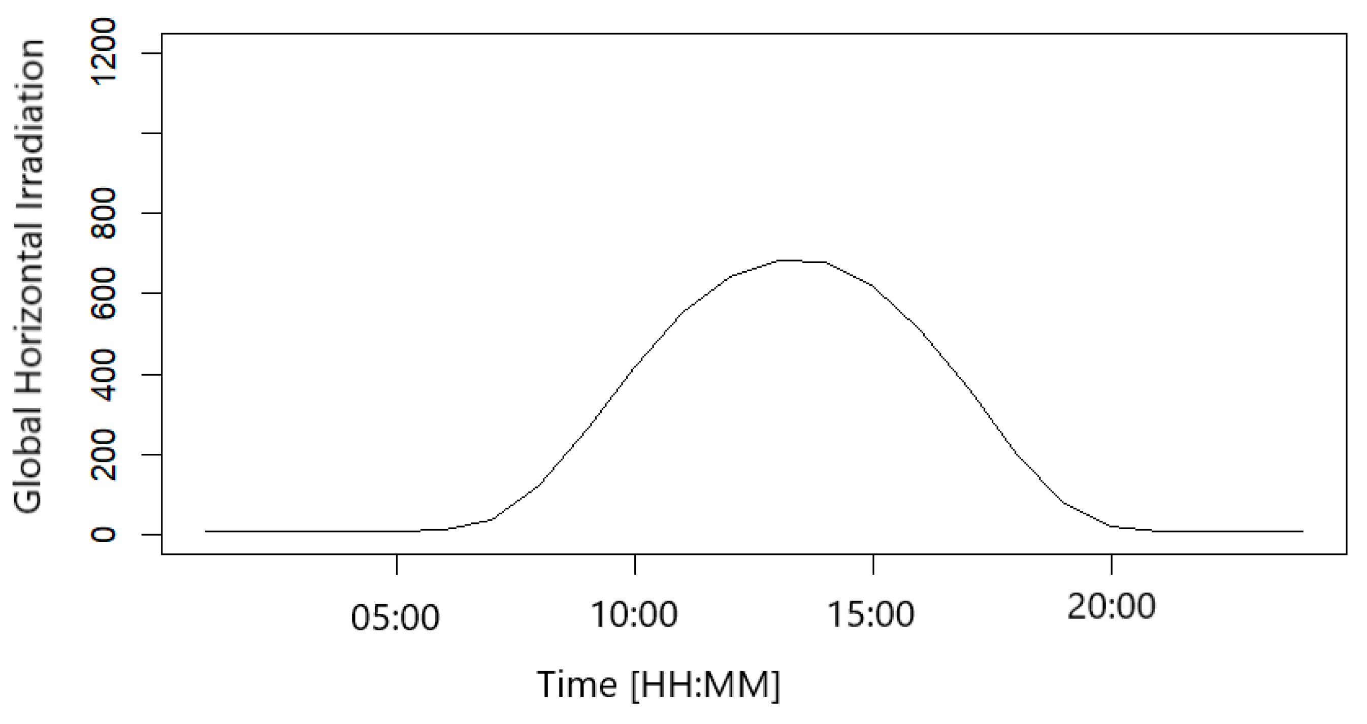
Solar irradiance (SI) for a particular day is significantly affected by the time horizon. This is supported by the time plots from all of the locations which have a general pattern shown in Figure 2. When measured in hours starting from midnight to midnight, [23] demonstrated that ignoring sidebands in the data causes overshoots just before sunrise and after sunset. As a result, we use up to 3 cycles per day which consider the sidebands.
Ref. [23] modelled this hourly profile for a particular day through a Fourier series. Thus, the mean function of SI in an hour for the three cycles in a day can be modelled as follows:
y t = β 0 + β 1 C o s ( π 12 t ) + β 2 S i n ( π 12 t ) + β 3 C o s ( 2 π 12 t ) + β 4 S i n ( 2 π 12 t ) + β 5 C o s ( 3 π 12 t ) + β 6 S i n ( 3 π 12 t ) + ε
The Fourier series expansion model should satisfy the following constraints:
  • ysunrise = ysunset = 0.
  • ysunrise−1hr = ysunset+1hr = 0.
As a result, this profile is considered on the QDFM of the SI hourly distribution such that we apply the following regression quantile distributional model as suggested by [2]:
Q y ( p | t ) = y t + η S ( p , α , γ , δ , τ ) t = 1 , 2 , 3 , , 24 .
where S(p, α, γ, δ, τ) is the basic quantile distribution function of the residuals (from the Fourier series expansion model in (11)) described by α, γ, δ and τ, the respective shape, scale, skewness and kurtosis parameters. We assume that E( ε ) = 0 and S(0.5) = 0. That is, the deterministic part of the distributional model in (12) becomes Galton’s median regression line. This means that
M [ S ( U r ) ]   =   S ( p * )   =   M r
which is called the median rankit for p* = IIB(0.5, r, n + 1 − r).

3.2.1. Venda and Gaborone Hourly Quantile Profiles

The ‘fitdistrplus’ R package developed by [24] automatically selects the best distribution that particular data follows. The package estimates the distribution parameters through a default maximum likelihood optimisation algorithm. As a result, the residuals on fitting the SI Fourier series for the Venda and Gaborone hourly profile followed a skew normal type 2 (SN2) distribution with the probability distribution parameters as estimated in Table 3. The ‘gamlss.dist’ R package developed by [25] was used to fit the distributions as shown in Figure A1. That is, the fitted QDFM is as shown in (14),
Q y ( p | t ) = β 0 + β 1 C o s ( π 12 t ) + β 2 S i n ( π 12 t ) + β 3 C o s ( 2 π 12 t ) + β 4 S i n ( 2 π 12 t ) + β 5 C o s ( 3 π 12 t ) + β 6 C o s ( 3 π 12 t ) + η { α + γ δ Φ 1 ( p ( 1 + δ 2 ) 2 ) , p ( 1 + δ 2 ) 1 α + γ δ Φ 1 ( p ( 1 + δ 2 ) 1 + δ 2 2 δ 2 ) , p > ( 1 + δ 2 ) 1 .
so that the model parameters are as shown in Table 4.

3.2.2. Durban, Pretoria, Cape Town and Windhoek Hourly Quantile Profiles

The residuals on Durban followed a skew exponential power type 3 distribution and the Cape Town and Windhoek profiles followed a sinh-arcsinh distribution. However, the skew exponential power type 3 and sinh-arcsinh probability distributions do not have corresponding quantile functions as yet. As a result, the closest alternative probability distribution is a normal or Cauchy distribution. The results in Table 5 show that the normal distribution better fits the residuals for the three locations than the Cauchy distribution. Thus, the fitted normal distributions (as second best fits) using the ‘fitdistrplus’ R package are shown in Figure A1.
The Durban and Cape Town residuals from the Fourier series model had means of −2.3122 × 10⁻¹⁶ and 1.1102 × 10⁻¹⁶ and standard deviations of 11.0653 and 13.4113 respectively. The residuals had also respective skewness of 0.051 and −0.055. As a result, the fitted QDFM is
Q y ( p | t ) = β 0 + β 1 C o s ( π 12 t ) + β 2 S i n ( π 12 t ) + β 3 C o s ( 2 π 12 t ) + β 4 S i n ( 2 π 12 t ) + β 5 C o s ( 3 π 12 t ) + β 6 C o s ( 3 π 12 t ) + η [ μ + σ Φ 1 ( p ) ] .
The residuals from the Windhoek and Pretoria deterministic models had a mean (µNUST = 0.2567696, µUP = −1.15597) and standard deviation of (σNUST = 21.3035529, σUP = 2.77733). However, the residuals from the Windhoek and Pretoria deterministic models have respective skewness of 0.162308 and −0.1442648, which cannot be ignored (that is, the skewness cannot be approximated to zero). That is, the residuals are suggesting some skewness, so considering a skewed lambda quantile distribution (in Equation (16)) for the residuals will give better results [21]. Therefore, we fit the following QDFM for the Pretoria and Windhoek hourly profiles. Thus, the estimated parameters are shown in Table 6.
Q y ( p | t ) = β 0 + β 1 C o s ( π 12 t ) + β 2 S i n ( π 12 t ) + β 3 C o s ( 2 π 12 t ) + β 4 S i n ( 2 π 12 t ) + β 5 C o s ( 3 π 12 t ) + β 6 C o s ( 3 π 12 t ) + η 2 σ [ ( 1 δ ) p σ ( 1 + δ ) ( 1 p ) σ ] .

3.2.3. Hourly Population Means

On average, the daily maximum irradiance was observed at 13:00 on all the stations considered, with either the second or third maximum taking place at 12:00 or 14:00. Using the hourly profile QDFMs fitted for each location, we can then estimate the population means at 12:00 up to 14:00 as follows:
μ t = 0 1 Q ( p | t ) d p , t = 12 , 13 , 14 .
Now, some QDFMs discussed in previous sections include the inverse cumulative distribution function (CDF) of the standard normal distribution, Φ−1(p). We adopt the method suggested by [26] of probabilistic polynomial approximations to evaluate the inverse. Researchers like [27,28] and the latest [29] concentrated on approximating the CDF. Ref. [29] are claiming to have the most accurate approximation using both the MATLAB Global Optimization Toolbox and BARON, but they did not document evaluating the inverse of the CDF. The approximation developed by [26] is explicit and has an acceptable maximum absolute percentage relative error (APRE) of 1.4 × 10⁻². We find their approximation function simple and very accurate for the purposes of estimating the population mean SI in any time interval of interest. Therefore, Table 7 shows the estimated population mean of the average SI for 12:00, 13:00 and 14:00 time hours at each location.
That is, for a period of 13:00 ± 2 h we can have an accumulative radiation of at least 3000 Wh/m2 which is the amount of energy required to fully charge a 12 Volt and 250 Amp solar battery. This means that given the correct solar panel capacity such a solar battery can be fully charged in at least five hours i.e., a period from 11:00 up to 15:00 at any of the locations in the Southern Africa region.

3.3. Daily Total SI Distributional Modelling

The daily total SI distribution is not that significantly influenced so much by other variables in such a way that it is not necessary to consider other meteorological features when modelling its quantile distribution. That is, a day’s total SI distribution for a particular month is presumed identical. The basic quantile functions S(p,α), considered on each month’s daily total fitted QDFMs at the locations under study are shown in Table 8. If we look at the population mean daily totals in Table 9, location by location then the maximums in a year were all received in summer (i.e., either November, December or January), except for Windhoek which has its maximum in autumn. The maximum population mean daily totals are shown in bold for each location. All locations receive their population mean daily total minimums in winter. Our results contrast with the conclusion drawn by [6] who had a maximum taking place in October and a minimum in January, though they analysed daily averages for Malawi.
We see it as not a proper descriptive analysis to consider the daily average because the minimum SI on every single day is always zero. In addition, SI is always approximately equal to zero from sunset progressing through the night up to sunrise. However, on some clear nights, we may have significant but very low SI readings. As a result, meaningful daily average analysis has to exclude readings from sunset up to sunrise when targeting the solar power generation industry. On the other hand, comparing the mean daily totals across the locations on each month Windhoek receives the maximum (daily population mean totals with an asterisk) in 75% of the year except for January, February and October. It is Cape Town, instead, which receives maximums in those other three months.

3.4. Monthly Total SI Distribution Modelling

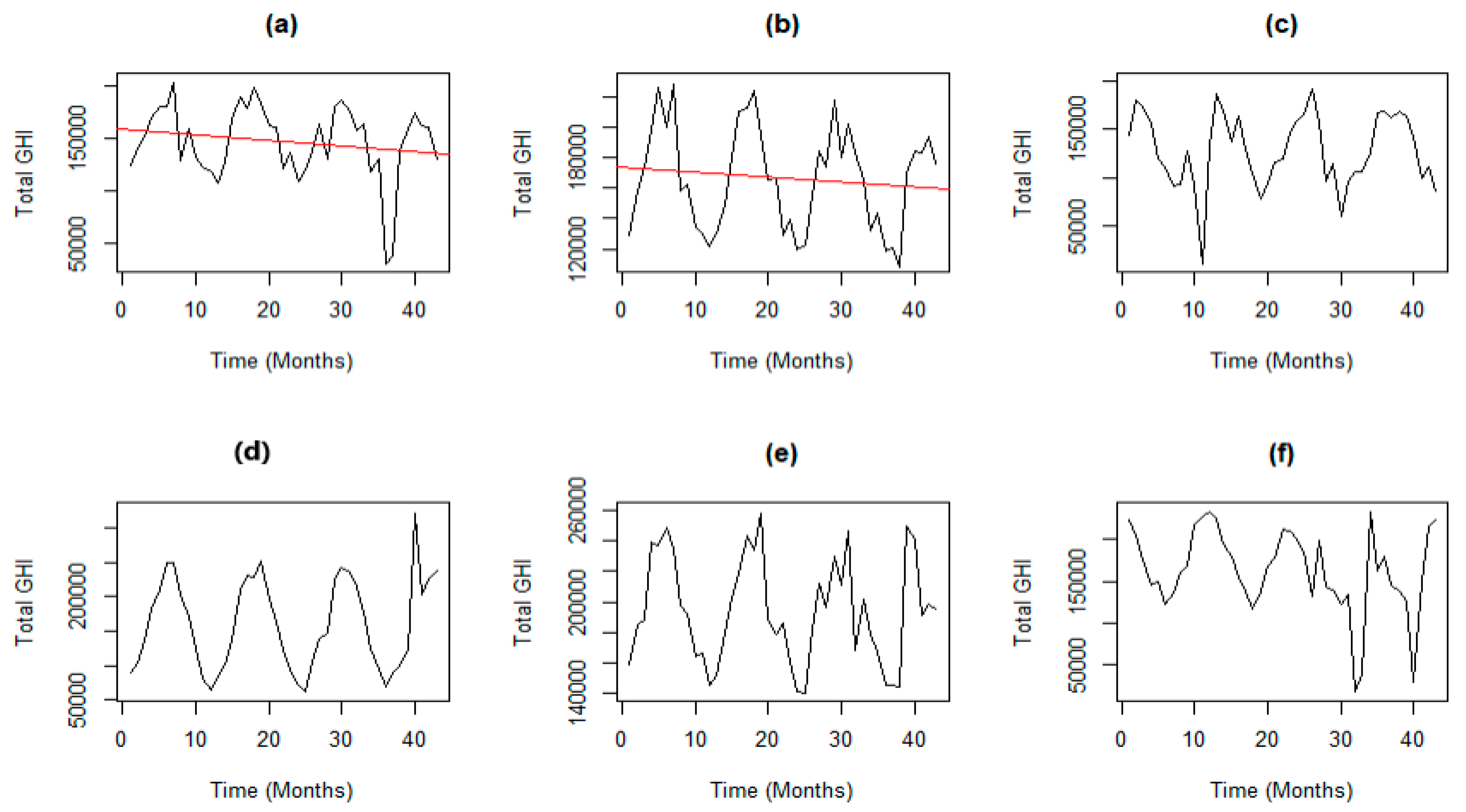
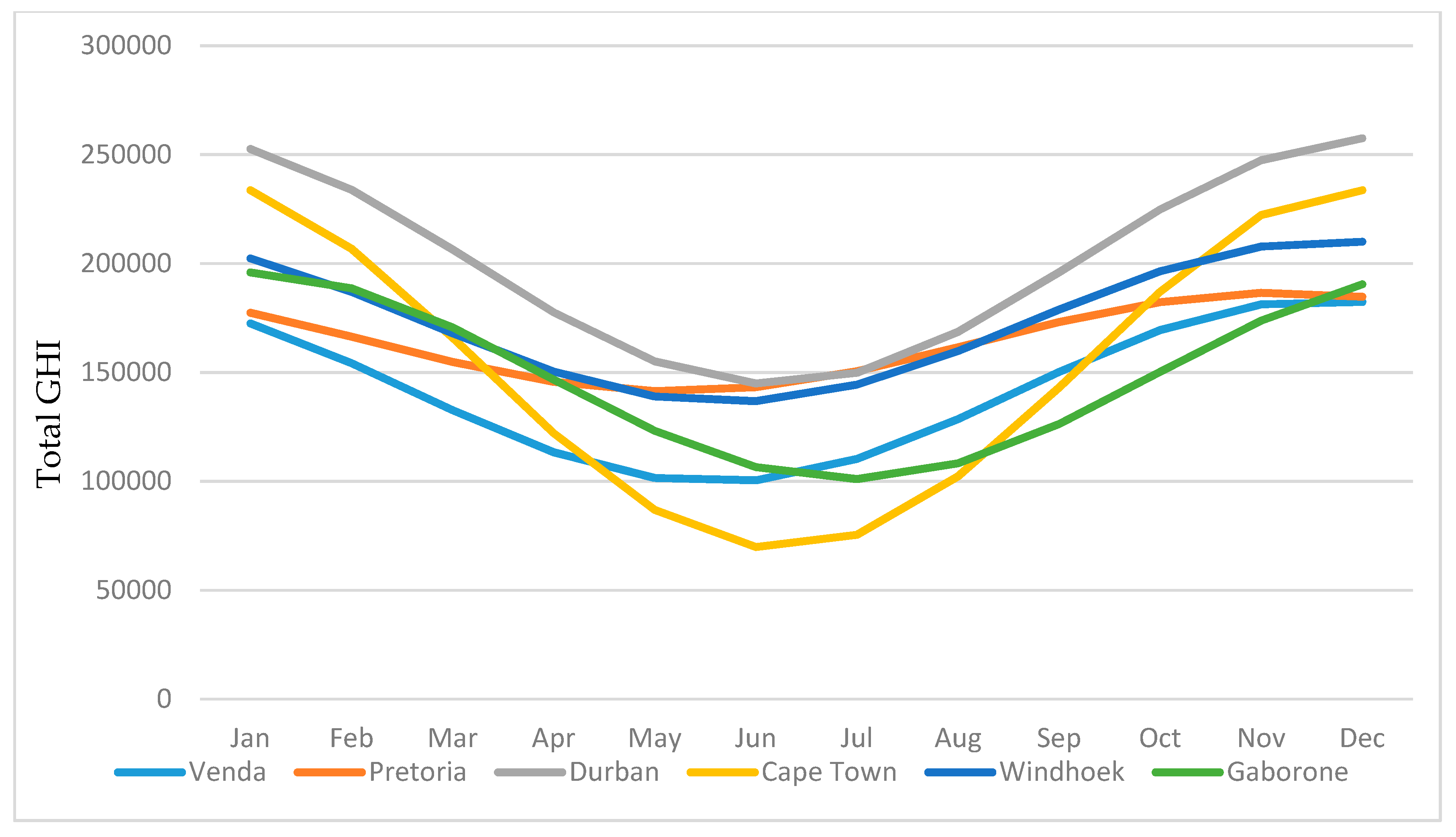
The monthly total SI for a particular year is significantly affected by the month. The deterministic component of monthly totals is suspected to be affected by the seasons of summer and winter because from Table 9 we can conclude that the daily population mean totals are affected by seasonal variation. This agrees with the results of [30], which showed that SI greatly changed its pattern according to seasonal variation. Figure 3 exhibits some cyclical variations in the monthly totals at all locations. As a result, we can attribute these cyclical variations to seasonal effects that were also discovered by [5,6,7] from different countries in Southern Africa. Thus, our cycle must have a period of 12 months. Therefore, we can fit the deterministic component of the monthly totals as the following trigonometric regression model:
y t = β 0 + β 1 C o s ( π 12 t ) + β 2 S i n ( π 12 t ) + ε
If a trend is observed on the time series plot of the monthly totals, then a trend component can be added to the deterministic model as follows:
y t = β 0 + β 1 t + β 2 C o s ( π 12 t ) + β 3 S i n ( π 12 t ) + ε .
Thus, the quantile distribution of the monthly totals can now be modelled as
Q y ( p | t ) = y t + η S ( p , α , γ ) ,
where S(p, α, γ) is the quantile distribution function of the residuals, ε , from the trigonometric regression model. However, the time series plots exhibited in Figure 3 show that we can suspect a trend in the Pretoria and Venda monthly totals’ time series, but fitting both the trigonometric regression models with and without a trend gave the results in Table 10. We can conclude that monthly total solar irradiance in the Southern African region is neither increasing nor decreasing. There is no significant trend in SI monthly totals from year to year. However, it is evident that due to global warming, atmospheric temperatures are increasing [31,32,33]. In contrast, our time series plots and model comparisons do not show that. Thus, the effects of global warming may not be influencing SI in the Southern African region. Rather, in variable selection concepts, the temperature is a significant explanatory variable for SI as demonstrated by researchers like [8,16,34,35] who had the meteorological feature as one of the important predictors of SI in their forecasting models. As a result, all of the QDFMs for the monthly totals are fitted without considering trend regression being part of the deterministic component.
The residuals for Cape Town and Durban followed sinh-arcsinh and skew exponential power type 2 distributions, respectively. Like the sinh-arcsinh distribution, the skew exponential power type 2 distribution does not have an existing quantile function. Likewise, we compare the closest two distributions to them as shown in Table 11. As a result, the better distribution was the normal distribution. Figure A4 shows the fitted normal distributions.
The residuals in the other locations were best fitted by the distributions shown in Table 12 and are also shown graphically as in Figure A4. Our results are in tandem with the results from [36]. The original residual distributions are different over the year and the day. However, because some distributions do not have existing quantile functions, Durban and Cape Town had the same second-best-fitted distribution over the day and the year. The fitted QDFMs for the monthly totals have the estimated parameters as shown in Table 12. All stations received maximum total population mean solar irradiation during summer and minimum in winter. These results agree with the seasonality in SI observed by researchers who studied the meteorological feature in Southern Africa. Durban is receiving the maximum total population mean all year round of all the locations considered, while the minimum is received in Cape Town (Figure 4). Therefore, Durban is the best location to set up a solar farm in the region when considering the monthly accumulated solar irradiation.

3.5. Model Validations

The Hosmer and Lemeshow (HL) goodness of fit test done on all of the fitted QDFMs had a p-value greater than 0.05 to indicate that all of the QDFMs were good fits to the respective data. In addition, a runs test on all the fitted models showed that the QDFMs were generating random fitted values except for the Venda and Gaborone monthly QDFMs. The Hosmer and Lemeshow p-values as well as those for the runs test are shown in Table 13.
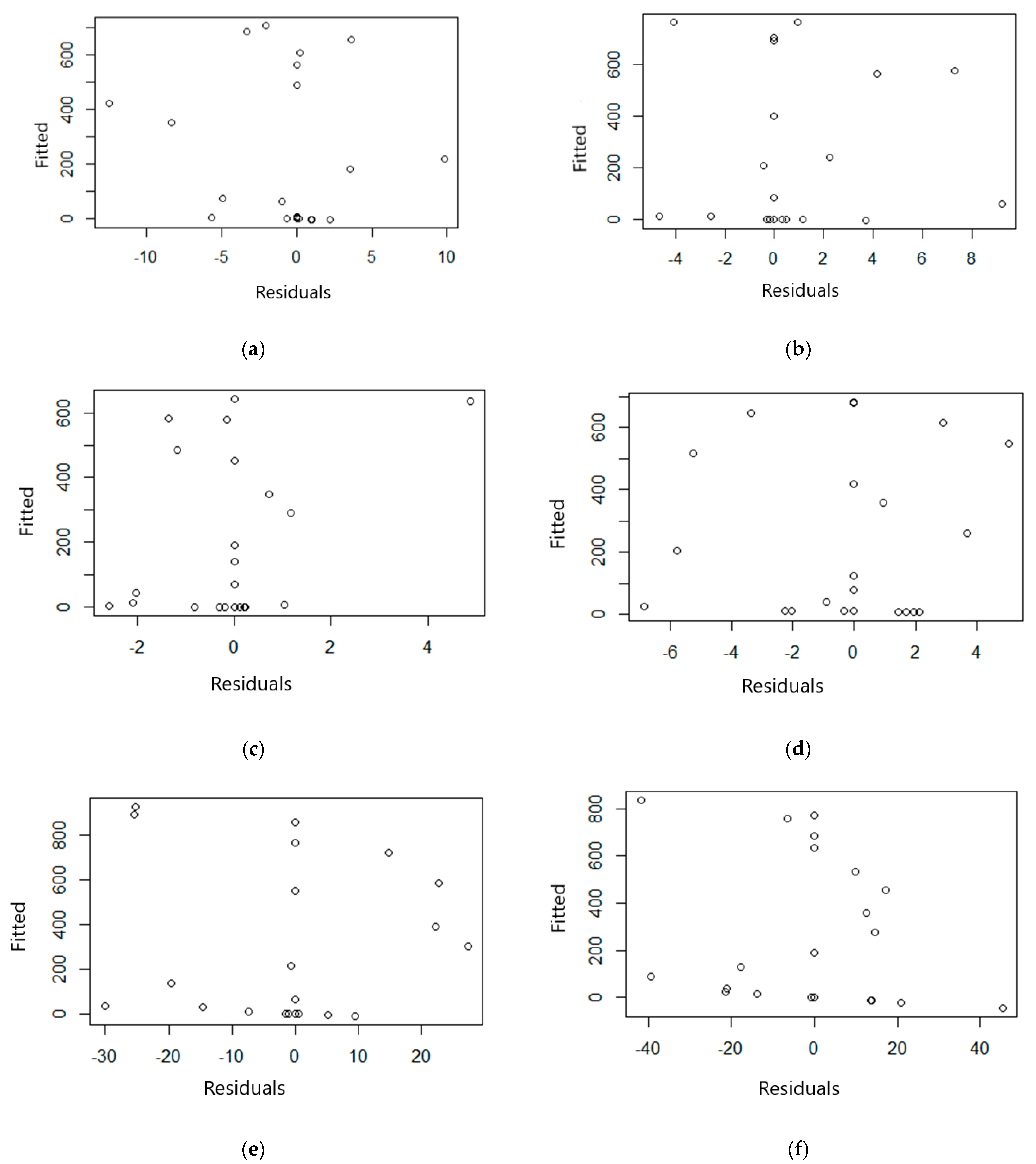
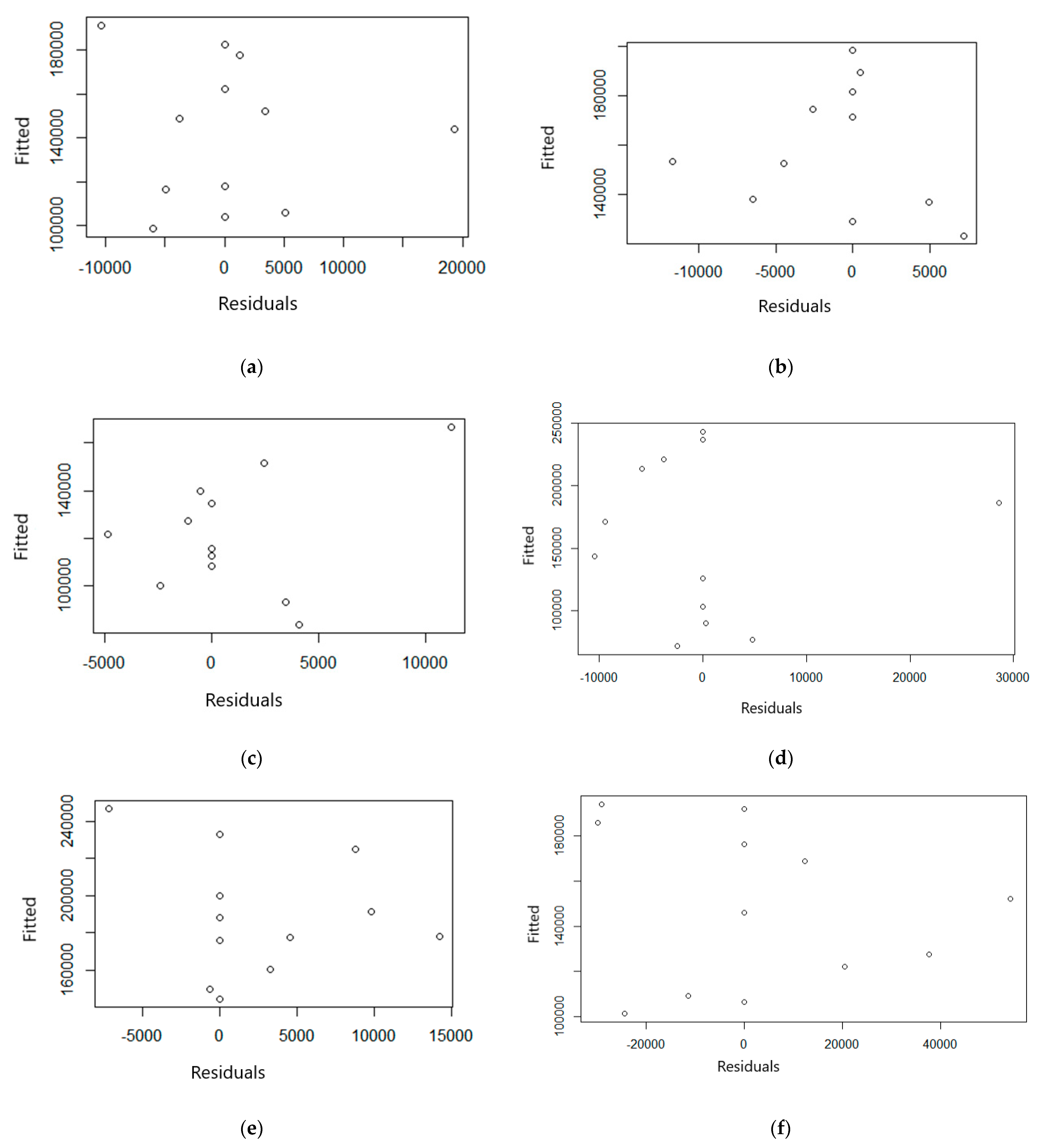
All of the fit-observation plots were approximately linear as shown in Figure A2 and Figure A5. All of the distributional residual plots did not exhibit any pattern. The points on the plots were haphazardly distributed on the scatter plots as shown in Figure A3 and Figure A6. Therefore, all of the fitted models are valid to use in describing the characteristics of solar irradiation in the locations studied.

4. Conclusions

The main objective of this study was not to predict but to explore the behaviour of SI using the unpopular quantile distributional functions modelling approach. The application of QFs has been shown to be a practical tool and gives more information than the use of only empirical distributions when exploring data. Both the deterministic and stochastic elements inherent in SI could be modelled on par to give a complete description of data characteristics. Application of the Fourier series in our residual analysis gave a direct physical interpretation of the deterministic component while QFs modelled the stochastic element. It enabled the representation of seasonality in the data when we considered different seasons. However, the seasonal modelling could be done over the year at once like the study from [37]. Therefore, the QDFM structure was developed by combining the two modelling components.
Although QDFMs are comprehensive and powerful data exploration tools, some probability distributions do not have existing QFs. This emerges as a drawback in accurately estimating the stochastic properties inherent in the data that follow such probability distributions. Therefore, further studies can be done on developing QFs of such probability distributions. Another challenge is approximating the inverse of the cumulative standardised normal distribution function. The approximations developed so far are complex. More studies can be done on simplifying the approximation process as well as increasing its accuracy.
Daily SI recorded on an hourly time horizon is cyclical, and that pattern can be modelled using a Fourier series. In the Southern African region, the meteorological feature is received on the earth’s surface at a maximum between 12:00 and 14:00 depending on seasonal variations, but on average the maximum is experienced during the 13th hour of the day throughout the whole year. Therefore, maximum solar power generation can be done within two hours of midday at any location in Southern Africa regardless of any weather conditions. Maximum daily totals are generally being received during summer (November, December and January) across the region except at Windhoek where the maximum true mean daily total is being received in autumn. We also conclude that Windhoek can be the best solar power generation location in the region when considering daily accumulated solar irradiation because it had the maximum daily population mean total in 9 months of the year, then followed by Cape Town. However, if we consider the monthly accumulated solar irradiance, then Durban is the best location to set up a solar farm in the region. All maximum monthly population mean totals are received at that location in the region. The monthly total SI across the region is a maximum in summer and a minimum in winter. This shows that SI is highly seasonal in the region. Therefore, we suggest that when forecasting SI in the region the modelling process should be split into summer models and winter models. Though seasonal in nature, we can also conclude that Southern Africa’s solar irradiance is not being influenced by global warming yet. With such solar irradiance climatic information, then, planners, designers and investors in the solar power generation industry can use this research when identifying where, when and how effective and efficient electricity generation can be operationalised in this region.
Finally, we acknowledge the availability of some meteorology approaches that can be used to further describe the climate of solar irradiation. Therefore, this research creates a starting platform for understanding solar irradiance climate in Southern Africa.

Author Contributions

Conceptualisation, A.M., D.M. and P.M.; methodology, A.M., D.M. and P.M.; software, A.M.; validation, A.M., D.M. and P.M.; formal analysis, A.M., D.M. and P.M.; investigation, A.M., D.M. and P.M.; resources, A.M.; data curation, A.M.; writing—original draft preparation, A.M.; writing—review and editing, A.M., D.M. and P.M.; visualisation, A.M., D.M. and P.M.; supervision, D.M. and P.M.; project administration, A.M. All authors have read and agreed to the published version of the manuscript.

Funding

This research received no external funding.

Data Availability Statement

The data used in this study are from Southern African Universities Radiometric Network (SAURAN), website (https://sauran.ac.za, accessed on 12 June 2022).

Conflicts of Interest

The authors declare no conflict of interest.

Appendix A

Appendix A.1. Fitted Probability Distributions on Modelling Residuals from Trigonometric Regression of the Hourly Profiles

Figure A1. Fitted residual distribution plot for (a) Venda; (b) Pretoria; (c) Durban; (d) Cape Town; (e) Windhoek; (f) Gaborone.
Mca 28 00086 g0a1

Appendix A.2. Hourly Profile QDFM Validation Plots

Figure A2. Fit-observation plot for (a) Venda; (b) Pretoria; (c) Durban; (d) Cape Town; (e) Windhoek; (f) Gaborone.
Mca 28 00086 g0a2
Figure A3. Distributional residual plots (a) Venda; (b) Pretoria; (c) Durban; (d) Cape Town; (e) Windhoek; (f) Gaborone.
Mca 28 00086 g0a3

Appendix B

Appendix B.1. Fitted Probability Distributions on Modelling Residuals from Trigonometric Regression of Monthly Totals
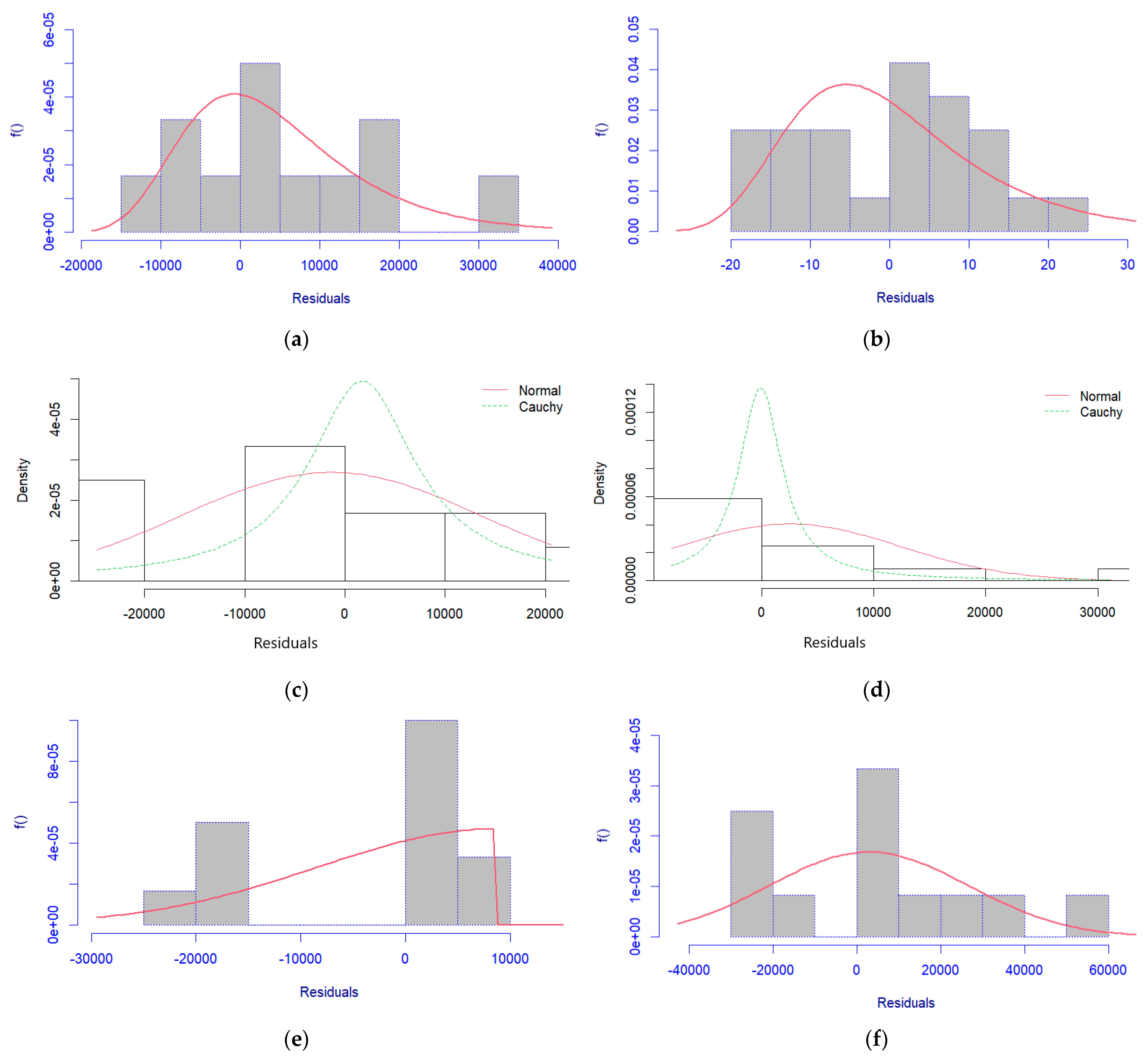
Figure A4. Fitted residual distribution plot for (a) Venda; (b) Pretoria; (c) Durban; (d) Cape Town; (e) Windhoek; (f) Gaborone.
Mca 28 00086 g0a4

Appendix B.2. Monthly Total Profile QDFMS Validation Plots

Figure A5. Fit-observation plots (a) Venda; (b) Pretoria; (c) Durban; (d) Cape Town; (e) Windhoek; (f) Gaborone.
Mca 28 00086 g0a5
Figure A6. Distributional residual plots (a) Venda; (b) Pretoria; (c) Durban; (d) Cape Town; (e) Windhoek; (f) Gaborone.
Mca 28 00086 g0a6

References

  1. Parzen, E. Quantile probability and statistical modelling. Stat. Sci. 2004, 19, 652–662. [Google Scholar] [CrossRef]
  2. Gilchrist, W.G. Regression Revisited. Int. Stat. Rev. 2008, 76, 401–439. [Google Scholar] [CrossRef]
  3. Yang, D. A universal benchmarking method for probabilistic solar irradiance forecasting. Sol. Energy 2019, 184, 410–416. [Google Scholar] [CrossRef]
  4. Jain, P.K.; Lungu, E.M.; Prakash, J. Stochastic characteristics of solar irradiation—Extremum temperatures processes. In Proceedings of the World Renewable Energy Congress VII (WREC 2002), Cologne, Germany, 29 June–5 July 2002. [Google Scholar]
  5. Jain, P.K.; Prakash, J.; Lungu, E.M. Correlation between temperature and solar irradiation in Botswana: Bivariate model. In Proceedings of the 2nd IASTED Africa Conference Modelling and Simulation (Africa MS 2008), Gaborone, Botswana, 8–10 September 2008. [Google Scholar]
  6. Salima, G.; Chavuka, G.M.S. Determining Angstrom constants for estimating solar radiation in Malawi. Int. J. Geosci. 2012, 3, 391–397. [Google Scholar] [CrossRef] [Green Version]
  7. Sivhugwana, K.S.; Ranganai, E. Intelligent techniques, harmonically coupled and SARIMA models in forecasting solar radiation data: A hybridisation approach. J. Energy South. Afr. 2020, 31, 14–37. [Google Scholar] [CrossRef]
  8. Mutavhatsindi, T.; Sigauke, C.; Mbuvha, R. Forecasting Hourly Global Horizontal Solar Irradiance in South Africa. IEEE Access 2020, 8, 19887. [Google Scholar] [CrossRef]
  9. Jain, P.K.; Lungu, E.M. Stochastic models for sunshine duration and solar irradiation. Renew. Energy 2002, 27, 197–209. [Google Scholar] [CrossRef]
  10. Jain, P.K.; Prakash, J.; Lungu, E.M. Climate characteristics of Botswana. In Proceedings of the Sixth IASTED International Conference, Gaborone, Botswana, 11–13 September 2006. [Google Scholar]
  11. Madhlopa, A. Study of diurnal production of distilled water by using solar irradiation distribution about solar noon. In Proceedings of the EuroSun 2006 Conference, Glasgow, Scotland, 27–30 June 2006. [Google Scholar]
  12. Madhlopa, A. Solar radiation climate in Malawi. Sol. Energy 2006, 80, 1055–1057. [Google Scholar] [CrossRef]
  13. Jain, P.K.; Lungu, E.M.; Prakash, J. Bivariate models: Relationships between solar irradiation and either sunshine or extremum temperatures. Renew. Energy 2003, 28, 1211–1223. [Google Scholar] [CrossRef]
  14. Govender, P.; Brooks, M.J.; Mathews, A.P. Cluster analysis for classification and forecasting of solar irradiance in Durban, South Africa. J. Energy South. Afr. 2018, 29, 1–6. [Google Scholar] [CrossRef]
  15. Bessafi, M.; Delage, O.; Jeanty, P.; Heintz, A.; Cazal, J.-D.; Delsaut, M.; Gangat, Y.; Partal, L.; Lan-Sun-Luk, J.-D.; Chabriat, J.-P.; et al. Research collaboration in solar radiometry between the University of Reunion Island and the University of Kwazulu-Natal. In Proceedings of the Third Southern African Solar Energy Conference, Mpumalanga, South Africa, 11–13 May 2015. [Google Scholar]
  16. Mpfumali, P.; Sigauke, C.; Bere, A.; Mlaudzi, S. Day Ahead Hourly Global Horizontal Irradiance Forecasting-Application to South African Data. Energies 2019, 12, 3569. [Google Scholar] [CrossRef] [Green Version]
  17. Ranganai, E.; Sigauke, C. Capturing Long-Range Dependence and Harmonic Phenomena in 24-Hour Solar Irradiance Forecasting. IEEE Access 2020, 8, 172204–172218. [Google Scholar] [CrossRef]
  18. Ratshilengo, M.; Sigauke, C.; Bere, A. Short-Term Solar Power Forecasting Using Genetic Algorithms: An Application Using South African Data. Appl. Sci. 2021, 11, 4214. [Google Scholar] [CrossRef]
  19. Chandiwana, E.; Sigauke, C.; Bere, A. Twenty-four-hour ahead probabilistic global horizontal irradiation forecasting using Gaussian process regression. Algorithms 2021, 14, 177. [Google Scholar] [CrossRef]
  20. Conde-Amboage, M.; Gonzalez-Manteiga, W.; Sanchez-Sellero, C. Quantile regression: Estimation and lack-of-fit tests. Bol. De Estad. E Investig. Oper. 2018, 34, 97–116. [Google Scholar]
  21. Gilchrist, W.G. Statistical Modelling with Quantile Functions; Chapman and Hall/CRC: Boca Raton, FL, USA, 2007. [Google Scholar]
  22. Karian, Z.A.; Dudewicz, E.J. Handbook of Fitting Statistical Distributions with R.; Chapman and Hall/CRC: Boca Raton, FL, USA, 2010. [Google Scholar]
  23. Boland, J. Time series modelling of solar radiation. In Modelling Solar Radiation at the Earth’s Surface: Recent Advances; Badescu, V., Ed.; Springer-Verlag: Berlin/Heidelberg, Germany, 2008; Chapter 11; pp. 283–312. [Google Scholar]
  24. Delignette-Muller, M.-L.; Dutang, C.; Pouillot, R.; Denis, J.-B.; Siberchicot, A. Package ‘fitdistrplus’. J. Stat. Softw. 2015, 24, 1–14. [Google Scholar]
  25. Stasinopoulos, D.M.; Rigby, A. Generalized additive models for location scale and shape (GAMLSS) in R. J. Stat. Softw. 2007, 23, 507–554. [Google Scholar] [CrossRef] [Green Version]
  26. Richards, W.A.; Antoine, R.; Sahai, A.; Acharya, M.R. An Efficient Polynomial Approximation to the Normal Distribution Function and Its Inverse Function. J. Math. Res. 2010, 2, 47–51. [Google Scholar] [CrossRef] [Green Version]
  27. Aludaat, K.M.; Alodat, M.T. A note on approximating the normal distribution function. Appl. Math. Sci. 2008, 2, 425–429. [Google Scholar]
  28. Soranzo, A.; Epure, E. Very Simply Explicitly Invertible Approximations of Normal Cumulative and Normal Quantile Function. Appl. Math. Sci. 2014, 8, 4323–4341. [Google Scholar] [CrossRef]
  29. Lipoth, J.; Tereda, Y.; Papalexiou, S.N.; Spiteri, R.J. A new very simply explicitly invertible approximation for the standard normal cumulative distribution function. AIMS Math. 2022, 7, 11635–11646. [Google Scholar] [CrossRef]
  30. Yan, K.; Shen, H.; Wang, L.; Zhou, H.; Xu, M.; Mo, Y. Short-Term Solar Irradiance Forecasting Based on a Hybrid Deep Learning Methodology. Information 2020, 11, 32. [Google Scholar] [CrossRef] [Green Version]
  31. Crowley, T.J. Causes of Climate Change Over the Past 1000 Years. Science 2000, 289, 270–277. [Google Scholar] [CrossRef] [Green Version]
  32. Argueso, D.; Evans, J.P.; Fita, L.; Kathryn, J. Temperature response to future urbanization and climate change. Clim. Dyn. 2014, 42, 2183–2199. [Google Scholar] [CrossRef]
  33. Chapman, S.; Watson, J.E.M.; Salazar, A.; Thatcher, M.; McAlpine, C.A. The impact of urbanization and climate change on urban temperatures: A systematic review. Landsc. Ecol. 2017, 32, 1921–1935. [Google Scholar] [CrossRef]
  34. Paulescu, M.; Tulcan-Paulescu, E.; Sudhansu, S.S. A temperature-based model for global solar irradiance and its application to estimate daily irradiation values. Int. J. Energy Res. 2011, 35, 520–529. [Google Scholar] [CrossRef]
  35. Mohanty, S.; Patra, P.K.; Sahoo, S.S. Prediction of global solar radiation using nonlinear autoregressive network with exogenous inputs (narx). In Proceedings of the 2015 39th National Systems Conference (NSC), IEEE, Greater Noida, India, 14–16 December 2015. [Google Scholar]
  36. Grantham, A.; Gel, Y.R.; Boland, J. Nonparametric short-term probabilistic forecasting for solar radiation. Sol. Energy 2016, 133, 465–475. [Google Scholar] [CrossRef]
  37. Boland, J. Characterising seasonality of solar radiation and solar farm output. Energies 2020, 13, 471. [Google Scholar] [CrossRef] [Green Version]
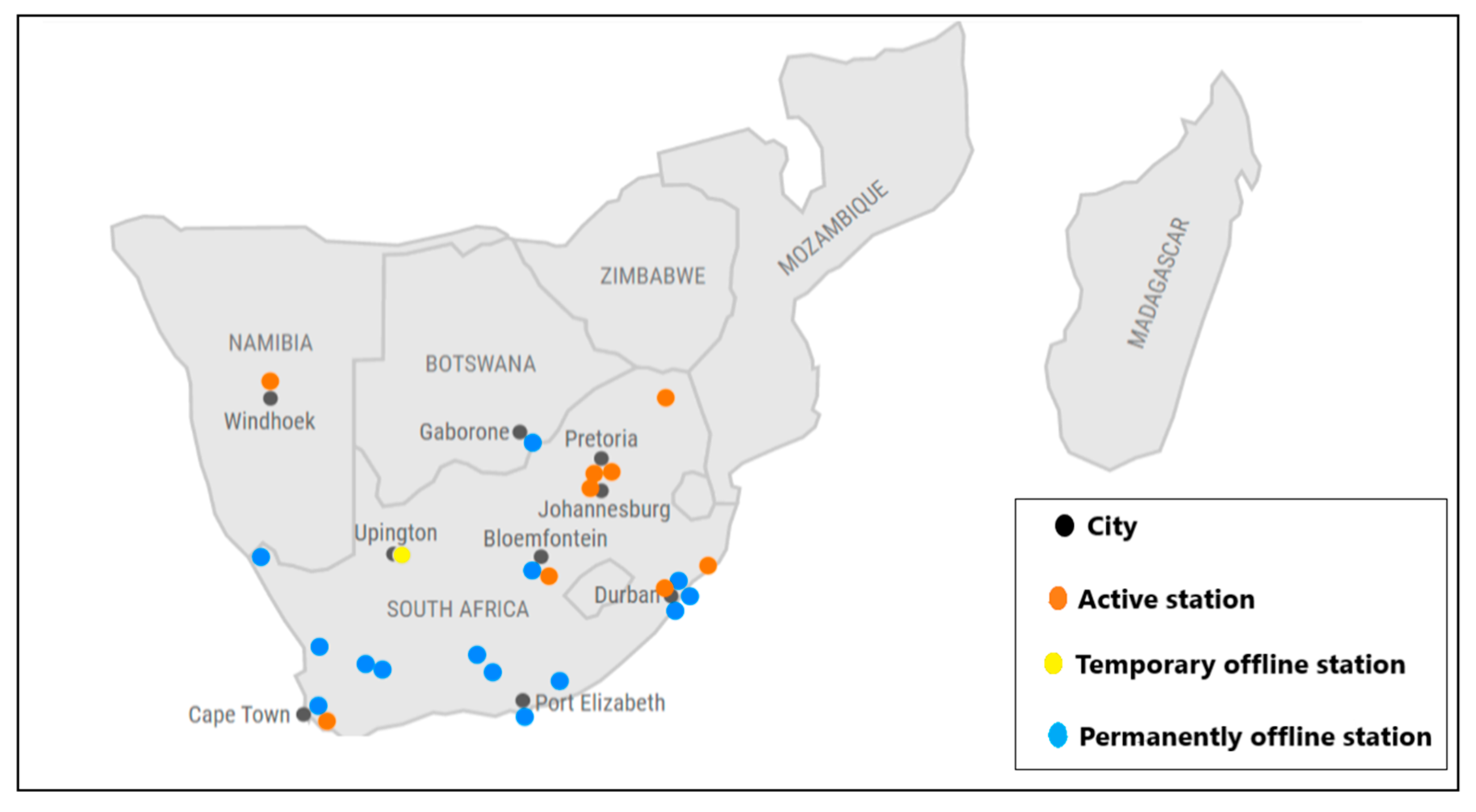
Figure 1. Radiometric Stations in Southern Africa (Source: www.sauran.ac.zw, accessed on 12 June 2022).
Mca 28 00086 g001
Figure 2. Day’s hourly profile.
Mca 28 00086 g002
Figure 3. Monthly total solar irradiation for (a) Venda; (b) Pretoria; (c) Durban; (d) Cape Town; (e) Windhoek; (f) Gaborone.
Mca 28 00086 g003
Figure 4. Monthly population mean totals (Wh/m2).
Mca 28 00086 g004
Table 1. QDFM validation plots.
Name of PlotyAgainstComment
Fit observationx(r)Q’(pr)Points to exhibit an approximately linear pattern
Distributional plotsfr = x(r) − Q’(pr)Q’(pr)Points to be randomly distributed
Table 2. SAURAN stations.
StationLatitudeLongitudeLocationPeriod
University of Venda (UV)−23.1310005230.42399979VendaApril 2015–April 2022
University of Pretoria (UP)−25.7530803728.22859001PretoriaJuly 2017–June 2021
University of KwaZulu-Natal Howard College (UKZNH)−29.8709793130.97694969DurbanDecember 2015–September 2022
Stellenbosch University (SUN)−33.9281005918.86540031Cape TownJuly 2017–June 2021
Namibian University of Science and Technology (NUST)−22.5650005317.07500076WindhoekJuly 2017–June 2021
University of Gaborone (UG)−24.660999325.93400002GaboroneJanuary 2015–November 2020
Table 3. Venda and Gaborone distributional parameters.
LocationShapeScaleSkewness
Venda22.676906−2.308079−5.612271
Gaborone23.2334042.127659−1.204687
Table 4. Venda and Gaborone model parameters.
Location β ^ 0 β ^ 1 β ^ 2 β ^ 3 β ^ 4 β ^ 5 β ^ 6 η ^
Venda143.24−327.52−55.60148.9057.37−17.3318.812.02
Gaborone422.36−372.09−92.34163.7371.42−16.13−6.71−8.17
Table 5. Residual fitted distribution comparisons.
LocationMetricNormalCauchy
DurbanAIC187.4920199.3287
BIC189.8481201.6848
Cape TownAIC196.7216211.7815
BIC199.077214.1376
WindhoekAIC218.9350222.8473
BIC221.2911225.2034
Table 6. Pretoria, Cape Town and Windhoek model parameters.
Location β ^ 0 β ^ 1 β ^ 2 β ^ 3 β ^ 4 β ^ 5 β ^ 6 η ^
Durban186.88−300.05−27.46145.5328.01−26.56−11.131.089
Cape Town220.88−309.44−111.00110.0391.52−6.93−11.831.034
Windhoek267.82−400.60−137.34159.85114.20−27.07−29.393676.63
Pretoria247.62−362.25−54.47163.3351.28−23.25−10.66−312.92
Table 7. 12:00–14:00 population means (Wh/m2).
Location12:0013:0014:00
Venda704.5501724.3324664.2824
Pretoria792.3848798.1858720.3530
Durban653.7334646.0031566.3265
Cape Town647.2710702.8115690.4624
Windhoek856.5969927.0284892.8881
Gaborone789.5647814.5785756.4473
Table 8. Probability distributions’ quantile functions.
Probability DistributionQuantile Function
Normal μ + σ Φ 1 ( p )
LognormalExp ( μ + σ Φ 1 ( p ) )
Skewed Lambda 1 2 σ ( ( 1 δ ) p σ ( 1 + δ ) ( 1 p ) σ )
Weibull α ( log ( 1 p ) ) 1 / γ
Gumbel α + γ log ( log ( 1 p ) )
Reverse Gumbel α γ log ( log ( 1 p ) )
Logistic α + γ log ( p 1 p )
Cauchy α + γ T a n ( π ( p 0.5 ) )
Weibull Type 3 β ( log ( 1 p ) ) 1 / γ
Table 9. Daily total population means (Wh/m2).
MonthVendaPretoriaDurbanCape TownWindhoekGaborone
January5808.486570.467419.848350.78 *7966.677045.33
February5118.635796.385569.627339.92 *6655.056741.43
March5328.465549.785727.715478.896969.69 *5847.43
April4218.164563.873869.334241.185855.68 *5143.91
May4189.184626.592832.393321.195183.17 *4593.42
June4207.394002.053543.302380.004946.30 *4292.30
July4463.094554.783146.753077.005109.11 *4522.42
August4338.575237.014393.843331.3310,342.86 *3966.38
September5820.816381.694684.334937.0010,678.41 *6310.75
October5441.116508.655773.347396.06 *7342.816881.60
November5992.287045.965197.027909.298022.61 *7370.91
December5786.877165.137118.958392.258799.95 *6856.38
Maximum5992.287165.137419.848350.7810,678.417370.91
Minimum4189.794002.052832.392379.964946.304292.30
* means a monthly maximum and bold means a locational maximum.
Table 10. Trend model AIC comparison.
LocationWithWithout
Venda266.7684265.613
Pretoria256.3586255.4424
Table 11. Comparisons of residual distributions on Cape Town.
LocationMetricNormalCauchy
Cape TownAIC187.4920199.3287
BIC189.8481201.6848
DurbanAIC268.5895271.3327
BIC269.5593272.3025
Table 12. Monthly total SI model parameters.
LocationProbability Distribution β ^ 0 β ^ 1 β ^ 2 η ^ α ^ γ ^
VendaR. Gumbel1,678,882.00−8767.1940,937.262013.06−768.989.11
PretoriaR. Gumbel3,692,969.00−9175.6820,756.984163.51−852.628.72
WindhoekSN2−24,798,121−5434.3536,610.502870.268700.05−0.69
LocationProbability Distribution β ^ 0 β ^ 1 β ^ 2 η ^ μ ^ σ ^
Cape TownNormal155,245.1112,380.0882,328.01−39.04−2.31 × 10−1611.06526
DurbanNormal197,409.843445.9537,525.342536.122488.449834.54
GaboroneNormal148,521.3322,150.6141,991.972372.42286323,670.46
Table 13. Goodness of fit test p-values.
LocationHourly QDFMMonthly QDFM
HLRuns testHLRuns test
Venda10.0949810.0154
Pretoria1110.2259
Durban10.403810.5431
Cape Town10.403810.2154
Windhoek10.403810.2259
Gaborone10.210510.0154
Disclaimer/Publisher’s Note: The statements, opinions and data contained in all publications are solely those of the individual author(s) and contributor(s) and not of MDPI and/or the editor(s). MDPI and/or the editor(s) disclaim responsibility for any injury to people or property resulting from any ideas, methods, instructions or products referred to in the content.