Abstract
Corrugated paperboard is a sandwich structure composed of wavy paper (fluting) bonded between two flat paper sheets (liners). The analysis of an entire package using three-dimensional numerical finite element models is computationally expensive due to the waved geometry of the board that requires the use of a relatively large number of elements in a simulation. Because of this, homogenisation approaches are used to evaluate equivalent homogenous models with similar material properties. These techniques have been successfully implemented by various researchers to evaluate the strength of corrugated paperboard. However, studies analysing the various homogenisation techniques and their ranges of applicability are limited. This study analyses the application of three homogenisation techniques: classical laminate plate theory, first-order shear deformation theory and deformation energy equivalence method in the evaluation of effective elastic material properties. In addition, inverse analysis has been applied to determine the effective properties of the board. Finite element models have been used to evaluate the accuracy of the three homogenisation techniques in comparison to the inverse method in modelling four-point bending tests and the results reported.
1. Introduction
Paperboard is an anisotropic structure consisting of two in-plane directions, namely, the machine direction (MD) and the cross direction (CD) which is perpendicular to the MD and the out-of-plane direction (ZD) [1]. Paperboard exhibits different properties in the MD, CD and ZD directions due to the fact that the fibers are aligned more in the flow direction (MD) during the manufacturing process [2,3,4].
Due to its light weight, affordability and high stiffness per unit weight, corrugated paperboard is the preferred material being widely used in the packaging industry for manufacturing packages [5,6,7]. FE (Finite Element) modelling is increasingly being used in the analysis of corrugated board packaging because it enables engineers to evaluate the performance of new package designs while eliminating the need for physical prototyping and experimental testing [6,7,8,9,10,11,12,13].
FE modelling has been employed by several researchers to evaluate the mechanical properties of corrugated paperboard, which include failure and collapse, creasing, stability and buckling [6,8,9,10,11,12,13,14,15,16]. The analysis of a complete package using three-dimensional(3D) models is computationally expensive and time-consuming due to the complex waved geometry of corrugated paperboard that necessitates the use of a high number of elements in the analysis. Due to these constraints, corrugated paperboard must be homogenised to a simple equivalent orthotropic laminate by replacing the waved geometry of the corrugated board with a two-dimensional (2D) laminate structure that represents the behaviour of the board [17].
Current homogenisation techniques applied for corrugated paperboard include classical laminate plate theory (CLPT), first-order shear deformation theory (FSDT) and the deformation energy equivalence method (DEEM). In these methods the properties of the individual kraft paper are used to analytically calculate the “homogenised” equivalent material properties for a laminate or single-layered board, which are then directly applied in the FE model [6,9,12,18,19].
Inverse analysis can also be applied in the homogenisation of corrugated paperboard. It has been applied by various researchers for model calibration [20,21,22], and involves evaluation of the optimal material model properties by using an FE model that duplicates the conditions of the physical test. It then calibrates the results by decreasing the difference between the numerical and experimental results. Studies highlighting the application of inverse analysis in the homogenisation of corrugated paperboard are limited. This study proposes the application of inverse analysis as a homogenisation technique for corrugated paperboard and seeks to evaluate the effectiveness of the homogenisation approaches highlighted above in finite element modelling of corrugated paperboard while comparing them to inverse analysis.
In this study, three homogenisation techniques, CLPT, FSDT and DEEM have been used to calculate the equivalent material properties of corrugated paperboard using material properties obtained from [7]. For CLPT and FSDT only the corrugated core was homogenised, and the board was modelled as a three-layered composite with two liners and a homogenised core. Using DEEM, the entire corrugated board was homogenised and modelled as a single-layered board. Inverse analysis has also been applied as a homogenisation method using structural and homogenised FE models of three-point bending (3PB) tests, and the objective function to be optimised was constructed from the difference between structural and homogenised tests force–displacement results. FE models and experimental tests have been used to analyse the accuracy of the above-mentioned homogenisation techniques in modelling the four-point bending (4PB) test.
2. Materials and Methods
2.1. Homogenisation of Corrugated Paperboard
This section discusses in detail the homogenisation approaches that were followed to determine the equivalent elastic properties of corrugated paperboard as a laminate structure and a single-layered board. The material properties were determined from tensile tests conducted on individual paper sheet samples of the C-flute board combination of 250KL/150SC/250KL and are presented in Table 1 [7]. The designations 250KL and 150SC refer to the paper grammages and types: 250 gsm (grams per square metre) virgin kraft liner and 150 gsm semi-chemical fluting paper. The out-of-plane elastic modulus, , was determined using Equation (1) [23]:
The shear moduli were determined using Equation (2) by [24]:

Table 1.
Measured elastic properties of individual paper sheets.
2.1.1. Classical Laminate Plate Theory
A method similar to those described by [6,7,25] was used to determine the equivalent material properties of the corrugated core. Strains and stresses of the corrugated core (fluting) were transformed using Equations (3) and (4) [6,7].
where and are strain and stress transformation matrices defined as Equations (5) and (6), respectively:
where c = cos() and s = sin() [6].
Because of the fluting’s waved geometry, the material properties for each section, , differ in the global coordinate system since the local system is constantly rotating. Therefore, the material properties, which were measured in the local coordinate system (123) have to be transformed to the global coordinate system . The fluting’s position can therefore be described as follows:
where is the distance from the centre line to the fluting, is the height of the fluting and P is the fluting’s wavelength (Figure 1). The rotation angle is calculated as follows:
The material compliance matrix, C, is built as a 3D matrix (Equation (9)) and rotated and reduced to a 2D matrix.
where is the material compliance matrix, E is Young’s modulus, is Poisson’s ratio and G is the shear modulus of the material, and 123 are the global and local coordinate systems of the material. The fluting is transformed from the local coordinate system to the global coordinate system using the transformation matrices in Equation (10).
The transformed matrices are given by Equation (11):
where Q is the plane stress material stiffness matrix. Using Kirchhoff–Love plate theory, in-plane strains can be disassembled into mid-plane strains and curvature (Equations (12) and (13)) since they vary linearly over the thickness of the element. Therefore, the strains at any distance z from the mid-plane is calculated as follows [25]:
while the laminar stresses are expressed using Hooke’s Law as
Integrating Equations (12) and (13) provides the in-plane normal, N, and bending moments, M, as shown in Equations (14) and (15):
where H is the board thickness. Equations (14) and (15) can be written alternatively:
where A is the extensional stiffness matrix, B is the bending-coupling stiffness matrix and D is the bending stiffness matrix obtained through integrating the thickness as shown in Equations (17)–(19) [7,25]:
where is the vertical thickness of the corrugated core calculated as follows:
and represents the thickness of the fluting (Figure 1). The stiffness of the board was then determined by integrating the section’s stiffness over an interval of the fluting’s period, P:
The above algorithm was applied in MATLAB and the resultant material properties obtained from homogenisation of the corrugated core are presented in Table 2.
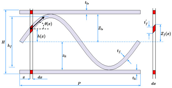
Figure 1.
Paperboard cross-section showing the front view of the top and bottom liners and the fluting. Here the subscripts , and f denote the top and bottom liner and fluting, respectively, while t is the thickness of each layer (Figure 1), Z represents the thickness direction coordinate of the liners and fluting with its origin on the centre line (mid-plane) [25].
Table 2.
Equivalent material properties of corrugated paperboard obtained from homogenisation.
2.1.2. First-Order Shear Deformation Theory
An approach similar to the method presented by [26] was used to determine the equivalent elastic properties of the corrugated core (fluting). The equation for a layer, k, in the laminate is expressed as Equations (22)–(25) [27]:
where are the mid-plane strains, and the bending curvatures, the twisting curvature and z the thickness-direction coordinate [26]. By differentiating in-plane stresses from transverse shear stresses and the strains described as mid-plane, flexural and transverse shear strains, the stress–strain relations can be written as shown in Equation (26) [6,19,27,28].
The resultant forces N, T and bending moments, M, are calculated by integrating the stresses through the thickness of each layer, and summing up the n, layers thus reducing the laminate from 3D to 2D [26,27]:
Consider the bending and twisting curvature and mid-plane and transverse shear strains are independent of z:
The stiffness matrices (Table A2) of the laminate are defined by Equations (34)–(37) [26]:
Here, represents the thickness of each layer and is the thickness direction coordinate of each layer. Considering Equations (34) to (37) the resultant forces and bending moments, they can be written in matrix form as follows:
The above algorithm was used to determine the equivalent elastic properties of the corrugated fluting using the measured material properties in Table 1. The material properties obtained from homogenisation of the corrugated core are presented in Table 2.
2.1.3. Deformation Energy-Equivalence Method
This is a numerical homogenisation method that is used to calculate the equivalent material properties of corrugated paperboard as a single layer as opposed to a laminate as described in CLPT and FSDT. It involves using an FE model of a representative volume element (RVE) to obtain the effective elastic properties of corrugated paperboard as proposed by [12,25,29]. For corrugated paperboard, RVE is an element whose total length is equal to the fluting’s wavelength and is modelled using shell elements to obtain the board’s stiffness [25]. The proposed method utilises the energy equivalence of the shell and the full RVE model to obtain the matrix of the board.
For this study the geometry of the RVE was created in Inventor Professional (Autodesk US, San Francisco, CA, USA, 2023), and the 0.5 mm square mesh of shell elements consisting of 1944 nodes (Figure 2) was generated using MSC Apex (MSC Software Corporation, Newport Beach, CA, USA, 2021). The geometry of a single wall corrugated paperboard with C flutes was developed by connecting three layers consisting of two liners and a fluting medium together. The connection between the liner and corrugated fluting was modelled by connecting the extreme positions of the fluting directly to the liners by sharing the same nodes. If none of the internal nodes are loaded, then Equation (39) is fulfilled:
where K is the stiffness matrix of external (boundary) degrees of freedom (DOFs) obtained using static condensation.
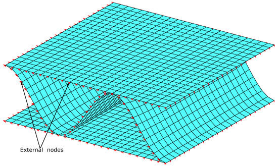
Figure 2.
RVE used in the energy-equivalence homogenisation technique showing the 248 external nodes used for evaluation of the global stiffness matrix.
The stiffness matrix was condensed to the outer edges of the RVE which consisted of 248 nodes with 5 degrees of freedom per node; x, y and z translation and rotation about the x and y axes. The overall stiffness matrix is expressed as follows [25]:
where subscripts e and i correspond to the external and internal degrees of freedom, respectively. Substituting into Equation (39) gives
The system’s total energy is given by Equation (42) [25]:
According to Kirchhoff–Love plate theory, if there is a constant strain distribution over an element, the relationship between the displacement of the node and strain of that node can be represented as shown in Equation (43) [25]:
where and the bending curvatures, the twisting curvature. Equation (43) can also be represented as:
where represents the displacement distribution over an element given the strains represented as Equation (45) for shell elements:
where ,, are the coordinates of the node of the FE model. Substituting Equations (42) and (44) gives Equation (46).
The internal energy of the shell subjected to bending is given by
Equating Equations (46) and (47) gives the matrix used to calculate the equivalent elastic parameters of the board:
MSC Marc was used to extract the global stiffness matrix and the coordinates of the external nodes from the RVE mesh applied in MATLAB to assemble the global stiffness matrix to a 1240 by 1240 matrix, which was used to calculate the general stiffness matrix (Table A3) of the corrugated board.
Structural and homogenised boards have different cross-sections, therefore the stress distribution along the thickness is altered in the process of homogenisation [17]. This implies that for a homogenised symmetric panel of thickness, t, only one of either the extensional, A, or bending matrices, D, will be represented correctly. To ensure that both matrices are recovered correctly, the effective thickness, , of the homogenised board is calculated as follows [17]:
2.2. Inverse Analysis
Inverse analysis makes use of a finite element model to duplicate the conditions of the experimental test first, and then optimises the material properties of the FE model by reducing the error between the experiments and the FE analysis [20].
In this study, structural and homogenised FE models of 3PB tests were set up to represent the physical and numerical tests, respectively. The objective function to be optimised was constructed from the differences between the 3PB structural and 3PB homogenised tests’ force–displacement results as shown in Equations (50) and (51).
MSC Marc was used for the FE analysis. Design Optimization Tools (DOT) [30], a gradient-based optimisation library for engineering applications was used for the optimisation. A python script that communicates with both DOT and MSC Marc was developed, and DOT was provided with the material properties of the FE model as variables to optimise. A Sequential Quadratic Programming (SQP) optimisation algorithm in DOT was employed to perform the optimisation. Figure 3 shows the numerical architecture that was used for the optimisation.
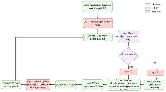
Figure 3.
Flow chart highlighting the optimisation process.
The 3D geometry of the corrugated board used to model the 3PB structural tests was created using Inventor Professional and the mesh generated using MSC Apex by joining the three layers, consisting of two liner-boards and a fluting medium. The adhesive between the liner and corrugated fluting was modelled by connecting the extreme positions of the fluting directly to the liners by sharing the same nodes. Figure 4 illustrates the developed mesh for the three-point bending models incorporating symmetry.
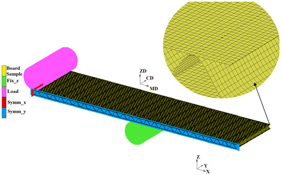
Figure 4.
Three-point MD bending test FE model with quarter symmetry.
Structural and homogenised finite element models were developed to simulate the 3PB tests (Figure 4), using MSC Marc. A linear elastic orthotropic material model was specified for the paperboard material and the material properties specified for the structural model obtained from Table 1. For the homogenised model, the equivalent material properties obtained from Table 2 were used. A four-node, shell element with six degrees of freedom per node x, y and z translation and rotation around the x, y and z axes was utilised for both models. The mesh convergence analysis converged to a 0.5 mm square mesh for the structural and a 2 mm square mesh for the homogenised models.
Symmetry conditions were applied using symmetry surfaces to model one-quarter of the experimental samples. The symmetry surfaces accounted for all the six rigid body motions, therefore no other boundary conditions were required. Two rigid bodies (cylinders) were used to represent the top-loading anvil and the bottom-fixed anvil similar to the experimental set-up (Figure 4). Load was applied using a downward position control on the top cylinder ramped up using a linear timetable and a static position control on the bottom cylinder. Load was applied incrementally using a multi-criteria adaptive stepping procedure to a total of 50 increments for each model. A full Newton–Raphson iterative procedure in which the model’s stiffness matrix is updated in each iteration was used to perform static analysis.
The root mean square error (RMSE) was used to estimate the error between the structural and homogenised FE model’s force–displacement results. The load extracted from the MD and CD structural FE models at each increment was denoted as and , respectively, while and represent the load extracted from the homogenised MD and CD FE models at each increment. Three RMSE values were calculated for each material direction, MD, CD and combined MD and CD, which can be seen in Equations (50), (51) and (53)
where i represents the current increment number and n is the total number of increments. The RMSE was not normalised for each material orientation (MD and CD) since the simulation terminated at a displacement of the same magnitude as shown in Figure 7 for each individual direction. The defined objective function, Equation (52) was subjected to two constraints, which were that the elastic moduli (, , ) in the FE models remain positive, and the FE analysis is valid by confirming an exit code of 3004 from MSC Marc. An exit code of 3004 implies that the simulation has been completed successfully.
Three different optimisation algorithms were used on three samples: individual MD and CD samples and combined MD and CD samples. This was performed so as to establish which numerical test was best for identification of certain parameters, for instance if is accurately determined in the CD test and in the MD test.
Homogenised material properties obtained from DEEM were used as the reference parameters from which 10 random starting points were generated using the latin hypercube function with the upper and lower limits chosen to be 20% above and below the reference points. Each of the starting points was first run through the FE analysis to ensure the constraints were satisfied before being submitted to DOT. The purpose of this was to determine if randomly generated starting points will converge to similar material properties (Table A4 and Table A5). All 10 optimisations were run simultaneously with the SQP algorithm in DOT. The optimal material properties were determined from the material model with the lowest objective function.
For the combined MD and CD optimisation, one RMSE value which represents the overall fit in both the MD and CD and the optimal solution was created by summing up the root mean square errors in both directions as shown in Equation (53):
2.3. Four Point Bending Experiment and FE Modelling
Structural and homogenised finite element models were developed to simulate four-point bending tests using MSC Marc (Figure 5 and Figure 6). An orthotropic material model was specified for the corrugated board and the properties in Table 1, Table 2 and Table 3 specified for structural and homogenised models, respectively. A four-node, shell element with six degrees of freedom per node (x, y and z translation and rotation around the x, y and z axes) was utilised. Bi-linear interpolation was used for coordinates, displacements and rotations during analysis, and strains and curvatures were calculated from the displacement and rotation fields, respectively. Transverse shear strains were computed near the edges and interpolated to the integration points. The mesh convergence analysis converged to a 0.5 mm square mesh for the structural model and 2 mm for the homogenised models (Figure 5 and Figure 6).
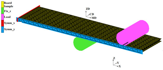
Figure 5.
Four-point MD bending test of structural FE model with quarter symmetry.
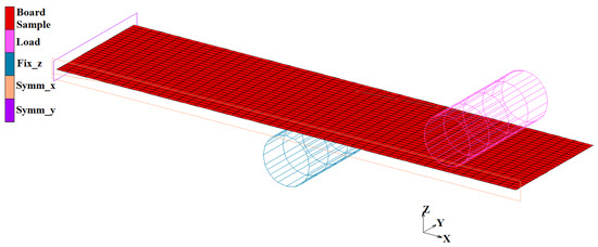
Figure 6.
Four-point MD bending test of homogenised FE model with quarter symmetry.
Table 3.
Equivalent material properties of corrugated paperboard obtained from inverse analysis.
Symmetry conditions were applied using symmetry surfaces to model one-quarter of the experimental samples. Two rigid bodies (cylinders) were used to represent the top-loading anvil and the bottom-fixed anvil similar to the experimental set-up (Figure 5). Load was applied using a downward velocity control on the top cylinder and a static position control on the bottom cylinder. Static analysis was performed using the full Newton–Raphson iterative procedure. The results from the analysis are summarised in Table 4.
Table 4.
Bending stiffness (N/m) comparison for four-point experimental and homogenised FE models.
For validation of the FE models, four-point bending stiffness experimental tests were conducted to determine the bending stiffness of board samples in the MD and CD according to ISO 5628 (1990) standard. Fourteen samples were tested on an Instron 5982 testing machine together with a HBM S2M (200 N) loadcell, HBM WA100 (100 mm) linear variable differential transducer (LVDT). The bending stiffness was calculated using Equation (54) [31] and the results are summarised in Table 4.
where P is the applied load, Y is the deflection at the centre of the specimen, L is the distance between supports, a is the distance between a support and loading point and b is the sample width.
3. Results and Discussion
This section provides a summary of the results obtained from homogenisation of corrugated paperboard, FE simulations of bending tests using the material properties obtained from standard homogenisation techniques and inverse analysis. A comparative analysis is done to determine the accuracy of standard homogenisation techniques and inverse analysis in predicting the strength of corrugated paperboard.
3.1. Homogenised Material Properties
Table 2 shows the equivalent material properties obtained using the three homogenisation techniques. The results show a good correlation to the values reported by [25,32] who applied both CLPT and DEEM homogenisation techniques on a similar C flute combination corrugated board.
From Table 2, the material properties obtained by DEEM indicate a much higher stiffness when compared to CLPT and FSDT because the entire sandwich structure of the corrugated board is homogenised to an equivalent single-layered board, while using CLPT and FSDT only the fluting is homogenised creating a three-layered laminate structure. The three homogenisation techniques applied cannot be used to obtain the equivalent plastic parameters of the board; however, they provide great starting points for application of optimisation algorithms. Table 3 shows the equivalent material properties obtained using inverse analysis.
From Table 3 it can be seen that the results obtained from using either the CD or MD models individually are not consistent. In the case of the MD model, the optimiser is not sensitive to , which is Young’s modulus in the cross direction, since the material is oriented in the direction of , this is the reason for the high standard deviation. Similarly, for the CD model, the value of has a high standard deviation showing that the optimiser is only sensitive to the values of . This implies that when running separate optimisations to obtain all three material properties, the optimiser is biased towards the principle material orientation of the specific model. In the case of the combined test, the obtained material properties have a much better consistency with acceptable standard deviations for the values of and , respectively. For all three cases, the optimiser is not sensitive to the value of due to the fact that the bending test does not initiate in-plane shear on the corrugated board.
3.2. Bending Tests
The material properties obtained using inverse analysis were verified by using them to model the 3PB test and comparing the homogenised models with experimental results as shown in Figure 7. From the results it can be seen that the inverse method accurately captured the linear deformation of the board when compared to the experimental results.
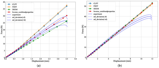
Figure 7.
Three-point bending force-displacement curves. (a) Comparison of MD force–displacement curves between FE models and experimental data. (b) Comparison of CD force–displacement curves between FE models and experimental data.
The results obtained from the inverse method were validated using four-point bending tests on the FE homogenised models and compared with the experimental results as presented in Figure 8. From Figure 8 it is quite clear that the material properties obtained from combined MD and CD algorithm provide an accurate prediction of the bending stiffness of the board when compared to the individual MD and CD algorithms.
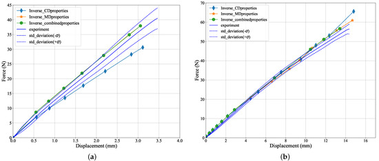
Figure 8.
Four-point bending force–displacement curves. (a) Comparison of MD force–displacement curves between FE models using parameters obtained from inverse analysis and experimental data. (b) Comparison of CD force–displacement curves between FE models using parameters obtained from inverse analysis and experimental data.
The results obtained from the four homogenised models were compared to 4PB experimental results to evaluate the accuracy of each technique in modelling the 4PB test when compared to experimental results. The R-Squared, (), (Equation (55)) was used to determine the percentage variation between the experimental results and the results predicted by the homogenised models. An value of 1 means that the predicted results perfectly fit the experimental results.
where is the experimental force, is the force predicted by the homogenised models and is the overall average force value obtained from the experimental results. Figure 9 and Table 4 show the correlation between the force–displacement curves of the homogenised FE models and experimental results.
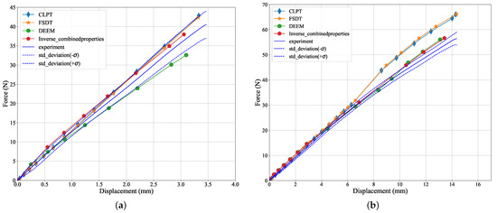
Figure 9.
Four-point bending force–displacement curves. (a) Comparison of MD force–displacement curves between FE models and experimental data. (b) Comparison of CD force–displacement curves between FE models and experimental data.
For all the homogenised models, the predicted bending stiffness was higher in the MD as compared to the CD for the four-point bending tests. From the results highlighted in Table 4 there was a good correlation between the bending stiffness values predicted by the homogenised models and experimental results for the four-point bending test with a difference of between 6% and 10% in the MD and 4% and 12% in the CD when compared with the experimental data. From the results in Figure 9, the four-point bending homogenised models can be used to predict the bending stiffness of the board with reasonable accuracy. Comparing the accuracy of the homogenisation methods in predicting the bending stiffness of the board from Table 4 and Figure 9, the inverse method was the most accurate in predicting the bending stiffness of the board.
4. Conclusions
In this study, four standard homogenisation techniques were presented, namely, CLPT, FSDT, DEEM and inverse analysis. The four techniques were applied in the elastic regime to determine the equivalent material properties of single-walled corrugated paperboard. CLPT and FSDT were implemented using a numerical integration script in MATLAB, while inverse analysis was applied using an optimisation algorithm. DEEM utilised an FE model of an RVE to evaluate the stiffness matrix of the board which allowed for inclusion of geometrical non-linearity in the computation of the matrix to a limited extent.
The four techniques were validated using experimental results of simple four-point bending tests. The bending stiffness values obtained from all the four methods were in agreement with the experimental results for the four-point bending tests with errors ranging between 4% and 12% for both the MD and CD directions.
The application of these homogenisation techniques is, however, limited to the elastic regime. In order to capture the plastic behaviour of the board other homogenisation techniques such as asymptotic homogenisation and multi-scale homogenisation need to be considered; however, they are computationally expensive. For this reason standard homogenisation techniques such as CLPT, FSDT, DEEM and inverse analysis are recommended since they are simple and do not require high computational power and the accuracy of the models is still within ±10%. From the four techniques that were analysed, inverse analysis provided the most accurate result when compared to CLPT, FSDT and DEEM and is therefore recommended as a homogenisation technique for corrugated paperboard.
Author Contributions
Conceptualisation, R.N.A., M.P.V. and C.J.C.; methodology, R.N.A.; software, R.N.A.; validation, R.N.A.; formal analysis, R.N.A.; data curation, R.N.A.; writing—original draft preparation, R.N.A., M.P.V. and C.J.C.; writing—review and editing, R.N.A., M.P.V. and C.J.C.; visualisation, R.N.A., M.P.V. and C.J.C.; supervision, M.P.V. and C.J.C.; project administration, M.P.V. and C.J.C. All authors have read and agreed to the published version of the manuscript.
Funding
This research was funded by the Stellenbosch University Postgraduate Scholarship Program.
Data Availability Statement
The data presented in this study are available on request from the corresponding author.
Conflicts of Interest
The authors declare no conflict of interest.
Appendix A. Stiffness Matrices Obtained from Homogenisation
Table A1.
Stiffness matrix for single-wall corrugated paperboard obtained from using CLPT [7].
Table A1.
Stiffness matrix for single-wall corrugated paperboard obtained from using CLPT [7].
| A & B | B & D | ||||||
|---|---|---|---|---|---|---|---|
| 1 | 2 | 3 | 1 | 2 | 3 | ||
| 1 | 1.18 | 0 | 0 | 0 | 0 | ||
| A & B | 2 | 2.43 | 0 | 0 | 0 | 0 | |
| 3 | 0 | 0 | 9.12 | 0 | 0 | 0 | |
| 1 | 0 | 0 | 0 | 0.34 | 0.07 | 0 | |
| B & D | 2 | 0 | 0 | 0 | 0.07 | 1.49 | 0 |
| 3 | 0 | 0 | 0 | 0 | 0 | 0.20 | |
Table A2.
Stiffness matrix for single-wall corrugated paperboard obtained from using FSDT.
Table A2.
Stiffness matrix for single-wall corrugated paperboard obtained from using FSDT.
| A & B | B & D | H | |||||||
|---|---|---|---|---|---|---|---|---|---|
| 1 | 2 | 3 | 1 | 2 | 3 | 4 | 5 | ||
| 1 | 0 | 0 | 0 | 0 | 0 | 0 | |||
| A & B | 2 | 0 | 0 | 0 | 0 | 0 | 0 | ||
| 3 | 0 | 0 | 0 | 0 | 0 | 0 | 0 | ||
| 1 | 0 | 0 | 0 | 1.01 | 0.23 | 0 | 0 | 0 | |
| B & D | 2 | 0 | 0 | 0 | 0.07 | 1.48 | 0 | 0 | 0 |
| 3 | 0 | 0 | 0 | 0 | 0 | 0.07 | 0 | 0 | |
| H | 4 | 0 | 0 | 0 | 0 | 0 | 0 | 0 | |
| H | 5 | 0 | 0 | 0 | 0 | 0 | 0 | 0 | |
Table A3.
Stiffness matrix for single-wall corrugated paperboard obtained from using DEEM.
Table A3.
Stiffness matrix for single-wall corrugated paperboard obtained from using DEEM.
| A & B | B & D | ||||||
|---|---|---|---|---|---|---|---|
| 1 | 2 | 3 | 1 | 2 | 3 | ||
| 1 | |||||||
| A & B | 2 | ||||||
| 3 | |||||||
| 1 | |||||||
| B & D | 2 | ||||||
| 3 | |||||||
Appendix B. Material Properties Obtained from Inverse Analysis
Table A4.
Equivalent material properties of corrugated paperboard obtained from inverse analysis conducted separately on MD and CD models.
Table A4.
Equivalent material properties of corrugated paperboard obtained from inverse analysis conducted separately on MD and CD models.
| MD | CD | ||||||||
|---|---|---|---|---|---|---|---|---|---|
| (MPa) | (MPa) | (MPa) | Optimal RMSE | (MPa) | (MPa) | (MPa) | Optimal RMSE | ||
| Reference properties (DEEM) | 797 | 442 | 182 | - | 797 | 442 | 182 | - | |
| 1 | 939.72 | 494.76 | 210.48 | 0.03 | 747.33 | 438.77 | 163.18 | 0.03 | |
| 2 | 939.58 | 499.11 | 215.53 | 0.03 | 885.18 | 441.56 | 172.86 | 0.03 | |
| 3 | 938.62 | 527.98 | 217.79 | 0.03 | 735.99 | 438.10 | 212.10 | 0.03 | |
| 4 | 941.20 | 477.57 | 157.01 | 0.03 | 800.63 | 440.25 | 178.58 | 0.03 | |
| Starting Points | 5 | 939.50 | 520.24 | 197.78 | 0.03 | 827.54 | 440.67 | 185.60 | 0.02 |
| 6 | 940.36 | 497.52 | 176.98 | 0.03 | 869.99 | 441.09 | 203.21 | 0.03 | |
| 7 | 941.95 | 429.07 | 182.52 | 0.03 | 850.88 | 441.27 | 157.75 | 0.03 | |
| 8 | 941.75 | 433.85 | 207.28 | 0.03 | 754.78 | 438.75 | 198.07 | 0.03 | |
| 9 | 940.73 | 499.01 | 160.38 | 0.03 | 750.76 | 438.28 | 206.69 | 0.03 | |
| 10 | 938.97 | 523.90 | 205.21 | 0.03 | 745.12 | 438.81 | 154.29 | 0.03 | |
| Average | 940.24 | 490.30 | 193.10 | 796.83 | 439.76 | 183.23 | |||
| Standard Deviation | 1.15 | 34.59 | 22.43 | 57.49 | 1.34 | 21.15 | |||
Table A5.
Equivalent material properties of corrugated paperboard obtained from inverse analysis of combined MD and CD models.
Table A5.
Equivalent material properties of corrugated paperboard obtained from inverse analysis of combined MD and CD models.
| Combined MD and CD | |||||
|---|---|---|---|---|---|
| (MPa) | (MPa) | (MPa) | Optimal RMSE | ||
| Reference Properties (DEEM) | 797 | 442 | 182 | - | |
| 1 | 940.54 | 441.88 | 193.06 | 0.05 | |
| 2 | 913.60 | 441.55 | 201.67 | 0.13 | |
| 3 | 940.88 | 442.15 | 173.63 | 0.05 | |
| 4 | 941.44 | 442.06 | 179.17 | 0.05 | |
| Starting Points | 5 | 940.44 | 442.07 | 210.35 | 0.05 |
| 6 | 941.47 | 442.24 | 158.87 | 0.05 | |
| 7 | 940.66 | 441.89 | 213.76 | 0.05 | |
| 8 | 941.46 | 442.15 | 166.30 | 0.05 | |
| 9 | 941.53 | 442.24 | 153.32 | 0.05 | |
| 10 | 940.88 | 441.90 | 184.79 | 0.05 | |
| Average | 938.29 | 442.01 | 183.49 | ||
| Standard Deviation | 8.68 | 0.21 | 21.05 | ||
References
- Hagman, A. Investigations of In-Plane Properties of Paperboard. Ph.D. Thesis, KTH Royal Institute of Technology, Stockholm, Sweden, 2013. [Google Scholar]
- Fadiji, T.S. Numerical and Experimental Performance Evaluation of Ventilated Packages. Ph.D. Thesis, Stellenbosch University, Stellenbosch, South Africa, 2019. [Google Scholar]
- Latka, J.F. Paper in architecture: Research by design, engineering and prototyping. A+ BE—Archit. Built Environ. 2017, 19, 1–532. [Google Scholar]
- Luong, V.D.; Abbès, F.; Abbès, B.; Duong, P.; Nolot, J.-B.; Erre, D.; Guo, Y.-Q. Finite element simulation of the strength of corrugated board boxes under impact dynamics. In Proceedings of the International Conference on Advances in Computational Mechanics, Phu Quoc Island, Vietnam, 2–7 August 2017; pp. 369–380. [Google Scholar]
- Harrysson, A.; Ristinmaa, M. Large strain elasto-plastic model of paper and corrugated board. Int. J. Solids Struct. 2008, 45, 3334–3352. [Google Scholar] [CrossRef]
- Talbi, N.; Batti, A.; Ayad, R.; Guo, Y. An analytical homogenization model for finite element modelling of corrugated cardboard. Compos. Struct. 2009, 88, 280–289. [Google Scholar] [CrossRef]
- Starke, M.M. Material and Structural Modelling of Corrugated Paperboard Packaging for Horticultural Produce. Ph.D. Thesis, Stellenbosch University, Stellenbosch, South Africa, 2020. [Google Scholar]
- Pathare, P.B.; Berry, T.M.; Opara, U.L. Changes in moisture content and compression strength during storage of ventilated corrugated packaging used for handling apples. Packag. Res. 2016, 1, 1–6. [Google Scholar] [CrossRef]
- Fadiji, T.; Ambaw, A.; Coetzee, C.J.; Berry, T.M.; Opara, U.L. Application of finite element analysis to predict the mechanical strength of ventilated corrugated paperboard packaging for handling fresh produce. Biosyst. Eng. 2018, 174, 260–281. [Google Scholar] [CrossRef]
- Beldie, L.; Sandberg, G.; Sandberg, L. Paperboard packages exposed to static loads– finite element modelling and experiments. Packag. Technol. Sci. Int. 2001, 14, 171–178. [Google Scholar] [CrossRef]
- Biancolini, M.; Brutti, C. Numerical and experimental investigation of the strength of corrugated board packages. Packag. Technol. Sci. Int. J. 2003, 16, 47–60. [Google Scholar] [CrossRef]
- Biancolini, M. Evaluation of equivalent stiffness properties of corrugated board. Compos. Struct. 2005, 69, 322–328. [Google Scholar] [CrossRef]
- Aboura, Z.; Talbi, N.; Allaoui, S.; Benzeggagh, M. Elastic behavior of corrugated cardboard: Experiments and modeling. Compos. Struct. 2004, 63, 53–62. [Google Scholar] [CrossRef]
- Gilchrist, A.; Suhling, J.; Urbanik, T. Nonlinear finite element modeling of corrugated board. In Proceedings of the the ASME Joint Applied Mechanicals and Materials Division Meeting, Blacksburg, VA, USA, 27–30 June 1999. [Google Scholar]
- Nordstrand, T. Parametric study of the post-buckling strength of structural core sandwich panels. Compos. Struct. 1995, 30, 441–451. [Google Scholar] [CrossRef]
- Allansson, A.; Svard, B. Stability and Collapse of Corrugated Board: Numerical and Experimental Analysis. Available online: https://lup.lub.lu.se/luur/download?func=downloadFile&recordOId=3566619&fileOId=3957829 (accessed on 12 February 2023).
- Garbowski, T.; Jarmuszczak, M. Homogenization of corrugated paperboard. Part 1. Anal. Homog. 2014, 70, 345–349. (In Polish) [Google Scholar]
- Buannic, N.; Cartraud, P.; Quesnel, T. Homogenization of corrugated core sandwich panels. Compos. Struct. 2003, 59, 299–312. [Google Scholar] [CrossRef]
- Duong, P.T.M. Analysis and simulation for the double corrugated cardboard plates under bending and in-plane shear force by homogenization method. Int. J. Mech. 2017, 11, 176–181. [Google Scholar]
- Jekel, C.F.; Venter, G.; Venter, M.P. Obtaining a hyperelastic non-linear orthotropic material model via inverse bubble inflation analysis. Struct. Multidiscip. Optim. 2016, 4, 927–935. [Google Scholar] [CrossRef]
- Gajewski, T.; Garbowski, T. Calibration of concrete parameters based on digital image correlation and inverse analysis. Arch. Civ. Mech. Eng. 2014, 14, 170–180. [Google Scholar] [CrossRef]
- Gajewski, T.; Garbowski, T. Mixed experimental/numerical methods applied for concrete parameters estimation. In Proceedings of the 20th International Conference on Computer Methods in Mechanics, Poznan, Poland, 27–31 August 2013; pp. 293–302. [Google Scholar]
- Mann, R.W.; Baum, G.A.; Habeger, C.C., Jr. Determination of All Nine Orthotropic Elastic Constants for Machine-Made Paper. Available online: https://smartech.gatech.edu/bitstream/handle/1853/3101/tps-084.pdf (accessed on 12 February 2023).
- Baum, G. Orthotropic elastic constants of paper. Tappi J. 1981, 64, 97–101. [Google Scholar]
- Marek, A.; Garbowski, T. Homogenization of sandwich panels. Comput. Assist. Eng. Sci. 2017, 22, 39–50. [Google Scholar]
- Suarez, B.; Muneta, M.L.M.; Sanz-Bobi, J.D.; Romero, G. Application of homogenization approaches to the numerical analysis of seating made of multi-wall corrugated cardboard. Compos. Struct. 2021, 262, 113642. [Google Scholar] [CrossRef]
- Berthelot, J.-M.; Ling, F.F. Composite Materials: Mechanical Behavior and Structural Analysis; Springer: Berlin/Heidelberg, Germany, 1999. [Google Scholar]
- Barbero, E.J. Introduction to Composite Materials Design; CRC Press: Boca Raton, FL, USA, 2010. [Google Scholar]
- Miehe, C.; Koch, A. Computational micro-to-macro transitions of discretized microstructures undergoing small strains. Arch. Appl. Mech. 2002, 72, 142–149. [Google Scholar] [CrossRef]
- Vanderplaats Research & Development Inc. DOT Users Manual, 5th ed.; Vanderplaats Research & Development Inc.: Colorado Springs, CO, USA, 2001. [Google Scholar]
- McKee, R.; Gander, J.; Wachuta, J. Compression strength formula for corrugated boxes. Paperboard Packag. 1963, 48, 149–159. [Google Scholar]
- Garbowski, T.; Jarmuszczak, M. Homogenization of corrugated paperboard. Part 2. Pol. Pap. Rev. 2014, 70, 345–349. (In Polish) [Google Scholar]


Disclaimer/Publisher’s Note: The statements, opinions and data contained in all publications are solely those of the individual author(s) and contributor(s) and not of MDPI and/or the editor(s). MDPI and/or the editor(s) disclaim responsibility for any injury to people or property resulting from any ideas, methods, instructions or products referred to in the content. |
© 2023 by the authors. Licensee MDPI, Basel, Switzerland. This article is an open access article distributed under the terms and conditions of the Creative Commons Attribution (CC BY) license (https://creativecommons.org/licenses/by/4.0/).