Article

A Bivariate Beta from Gamma Ratios for Determining a Potential Variance Change Point: Inspired from a Process Control Scenario

by
Schalk W. Human
1,
Andriette Bekker
1,2,*,
Johannes T. Ferreira
1,2 and
Philip Albert Mijburgh
1
1
Department of Statistics, University of Pretoria, Pretoria 0002, South Africa
2
Centre of Excellence in Mathematical and Statistical Sciences, Johannesburg 2000, South Africa
*
Author to whom correspondence should be addressed.
Math. Comput. Appl. 2022, 27(4), 61; https://doi.org/10.3390/mca27040061
Submission received: 2 June 2022 / Revised: 10 July 2022 / Accepted: 14 July 2022 / Published: 16 July 2022
(This article belongs to the Special Issue Computational Mathematics and Applied Statistics)

Abstract

:
Within statistical process control (SPC), normality is often assumed as the underlying probabilistic generator where the process variance is assumed equal for all rational subgroups. The parameters of the underlying process are usually assumed to be known—if this is not the case, some challenges arise in the estimation of unknown parameters in the SPC environment especially in the case of few observations. This paper proposes a bivariate beta type distribution to guide the user in the detection of a permanent upward or downward step shift in the process’ variance that does not directly rely on parameter estimates, and as such presents itself as an attractive and intuitive approach for not only potentially identifying the magnitude of the shift, but also the position in time where this shift is most likely to occur. Certain statistical properties of this distribution are derived and simulation illustrates the theoretical results. In particular, some insights are gained by comparing the newly proposed model’s performance with an existing approach. A multivariate extension is described, and useful relationships between the derived model and other bivariate beta distributions are also included.

1. Introduction

1.1. Problem Contextualisation

The monitoring of the variance of independent and identically distributed (i.i.d) normal random variables over time by taking successive, independent samples of measurements over time remains an interesting and valuable research consideration within quality control environment. In this case, when the variance σ 2 changes to σ 1 2 = λ σ 2 for some λ 1 , the practitioner needs to investigate the scope of such a change (a value of λ ), and ideally, the position within the successive measurements where such a change could’ve taken place. Suppose that X i j are i.i.d. N ( μ , σ 2 ) , i = 0 , 1 , 2 , , κ 1 and X i j i.i.d. N μ , σ 1 2 = λ σ 2 , i = κ , κ + 1 , , m where j = 1 , 2 , , n i 2 and λ > 0 , as outlined in Figure 1. The values of κ and λ are assumed to be unknown, but deterministic in nature. The order of these samples is important and cannot be re-ordered; in other words, the samples have a set sequence corresponding to the order in which they were obtained.
Thus, inspired by a practical objective, this paper aims to present a theoretically motivated framework to
  • present and contextualise this problem within the quality control environment;
  • follow a systematic approach to build up the distributional foundations from this practical perspective;
  • exploratively focus on the development of the (new) resulting bivariate beta distribution;
  • compare this model with an existing approach; and
  • determine whether λ 1 , and if this is indeed the case, to determine κ , the location of where the shift in the variance occurred.
Therefore, from sample κ onwards, the process would be considered out-of-control. Note that it is assumed that the shift occurs between two samples.
Assume that both the process mean ( μ ) and variance σ 2 are unknown, and that they are estimated by their respective minimum variance unbiased estimators (MVUE), given by:
X ¯ i = j = 1 n i X i j n i , i = 0 , 1 , 2 , , m ,
S i 2 = 1 n i 1 j = 1 n i X i j X ¯ i 2 , i = 0 , 1 , 2 , , m ,
where X ¯ i and S i 2 denote the mean and variance of sample i respectively. Some particular notes on Equation (1) and (2) include:
  • The index variable i ranges from 0 to m: a total of m + 1 independent rational subgroups or samples.
  • At least two samples are needed for a potential shift between them to be possible, therefore we assume m 1 .
  • The sample size n i can vary between different samples.
  • n i 2 is necessary since the process mean and variance are both assumed to be unknown and have to be estimated.
  • The pooling approach here is to use m r + 1 and r sample means and variances in the construction of the test statistic in Section 1.2. Alternatively one can consider a single mean/variance in this construction, which would result in additional information i = r m n i 1 and i = 0 r 1 n i 1 such that n i 1 and probability density functions are valid. In this case, the approach would reduce to a two sample comparison testing for a change in the variance.
The problem of determining if a shift in the process variance has occurred can be divided into two stages, namely before the potential shift and after, as indicated below ( G a m m a ( · , · ) denotes the usual gamma distribution with suitable shape and scale parameters [1]).
Mca 27 00061 i001

1.2. A Solution: Sequential Statistic Framework

The proposed distribution compares all the sample variances before a certain point (where the potential shift occurs), with all sample variances after the time of the shift. In essence, the multi-sample hypothesis testing problem is approached by using m sequential two sample tests; described as:
S 0 2 is compared with S 1 2 , S 2 2 , , S m 2 S 0 2 , S 1 2 is compared with S 2 2 , S 3 2 , , S m 2 and so forth until S 0 2 , S 1 2 , , S m 1 2 is compared with S m 2 .
Note that, due to the assumption that we have m + 1 samples, the procedure to identify the possible change in the variance requires m comparisons. Of these m comparisons the one that leads to the largest disparity between the sample variables on the left and the right of (5) will indicate the most likely position where the process experienced a change in variance. In essence, what is then needed is to quantify the difference between the sample variances of the left and right of (5), and then determine which of the m different comparisons has the largest difference between the sample variances, and finally to use some measure to determine if this maximum difference is within some set tolerance range. Our proposed mathematical construct on how to achieve this is discussed for the remained of this introduction. Assuming that no shift in the process variance has occurred, it is possible to construct a series of two sample statistics that correspond to the general procedure described in (5). Each statistic corresponds to whether at sample r = κ the two independent samples (the sample variances before time r and the sample variances after and including time r) are from normal distributions with the same unknown variance σ 2 . This can alternatively be viewed as testing whether σ 2 = σ 1 2 , which is similar to testing λ = 1 . As such, it follows that detecting a shift in the process variance can be reduced to the following hypothesis test:
H 0 : σ 2 = σ 1 2 vs . H A : σ 2 σ 1 2 or alternatively H 0 : λ = 1 vs . H A : λ 1 .
Suppose that a shift of size λ occurs in the process variance, then the corresponding random variables after the shift would be W i G a m m a ( n i 1 2 , 2 λ ) , i = κ , κ + 1 , , m distributed (see (4)). If there is no shift in the variance, λ = 1 , and it follows that W i G a m m a ( n i 1 2 , 2 ) , i = 0 , 1 , , m . Thus the hypothesis being investigated can be changed depending on the choice of the scale parameter of the specific gamma random variables. From (5) it follows that the series of statistics that forms the building blocks of the process are given by
U r * = i = r m n i 1 S i 2 λ σ 2 i = r m n i 1 i = 0 r 1 n i 1 S i 2 σ 2 i = 0 r 1 n i 1 i = r m W i i = r m n i 1 i = 0 r 1 W i i = 0 r 1 n i 1 , r = 1 , 2 , , m 1 , m ,
where W i G a m m a ( n i 1 2 , 2 ) for i = 1 , 2 , , r 1 and W i G a m m a ( n i 1 2 , 2 λ ) for i = r , r + 1 , , m .
In essence, (6) implies that the sample variances before the potential shift are pooled together, and the sample variances after the potential shift are pooled together. The numerator of the statistic at time r is the average, weighted by each statistic’s degrees of freedom, of all the sample variances between and including samples r and m, while the denominator is the corresponding weighted average of all the sample variances between and including samples 0 and r 1 ; this is graphically presented in Figure 2. Thus U r * is the test statistic that is typically used to test the equality of two population variances from a normal distribution.
From (3), (3) and (6), it follows that if no shift has occurred in the process variance, i.e., λ = 1 , each statistic U r * is univariate F distributed with i = r m n i 1 and i = 0 r 1 n i 1 degrees of freedom, respectively.
The reasoning behind the critical values that would indicate whether λ 1 is justified by inspecting the sequence of statistics in (6). Suppose that an increase λ > 1 in the process variance has occurred from sample r = κ onward, then:
  • The statistic U r * ’s numerator will contain only sample variances that come from a N μ , λ σ 2 , λ > 1 distribution, whereas the denominator will contain only sample variances that come from a N μ , σ 2 distribution.
  • If k 1 is some integer value such that 1 r k 1 < r , then the statistic U r k 1 * will contain k 1 sample variances in its numerator that are from a N μ , σ 2 distribution. This will reduce the weighted average of the sample variances of U r k 1 * ’s numerator in comparison to the numerator of U r * .
  • Similarly, if k 2 is some integer value such that r < r + k 2 m , then the statistic U r + k 2 * will contain k 2 sample variances in its denominator that are from a N μ , λ σ 2 distribution. This will increase the weighted average of sample variances of U r + k 2 * ’s denominator in comparison to the denominator of U r * .
  • Thus, any statistic other than the one immediately following the shift in the process variance, will contain either smaller sample variances in its numerator, or larger sample variances in its denominator (on average). Either of these scenarios result in a high probability that all other statistics are smaller relative to U r * .
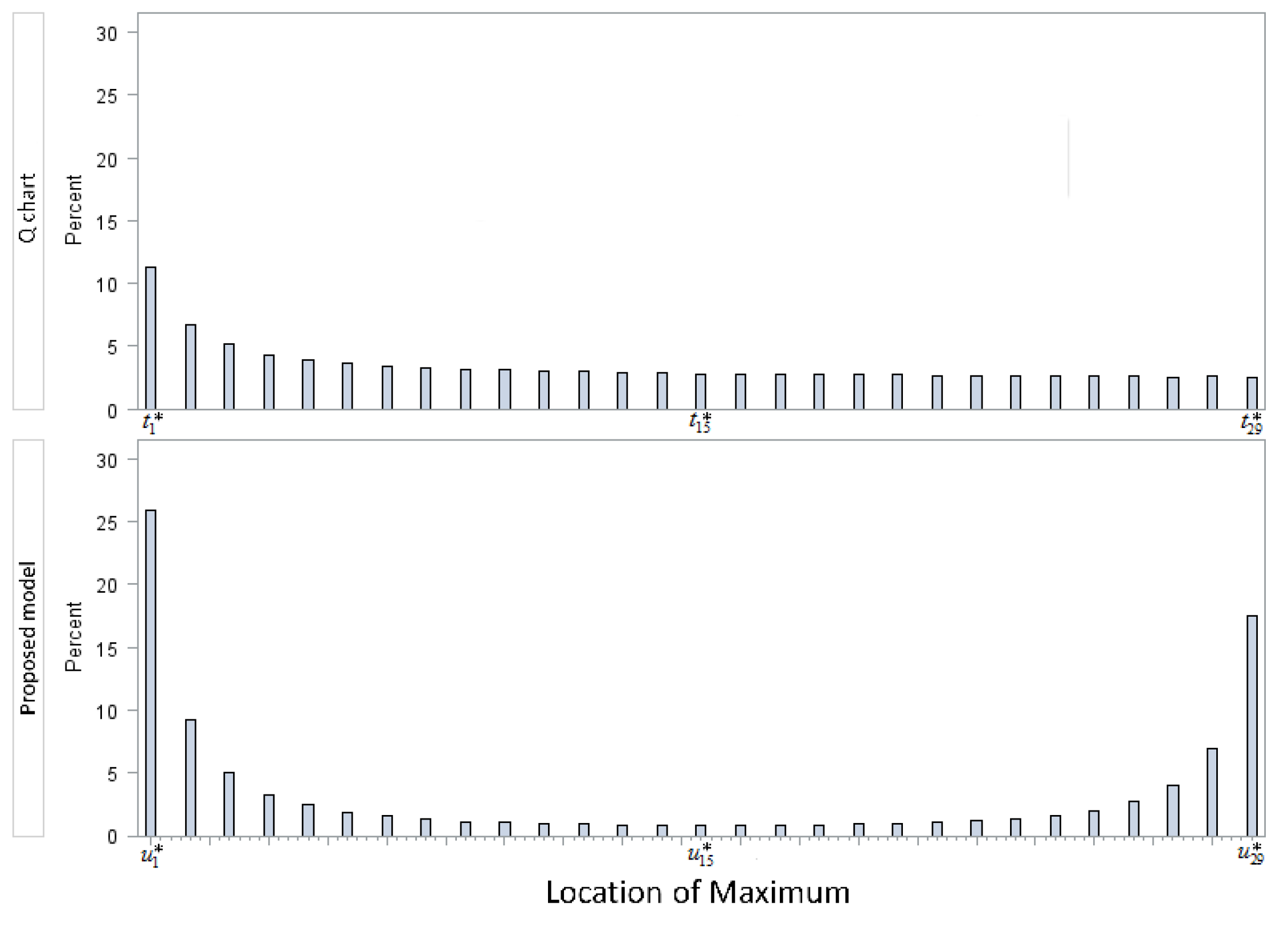
  • This leads to the conclusion that the most probable place where an upwards shift in the process variance will be detected is at the statistic immediately following the shift. The value that this statistic assumes also has a high likelihood of being the maximum value of all the U r * , r = 1 , 2 , , m 1 , m statistics.
  • As such, the most reasonable method of calculating the critical value to detect an upwards shift in the process variance is to calculate the maximum order statistic of the charting statistics U r * , r = 1 , 2 , , m 1 , m , (under the null hypothesis) and to set the critical value equal to some percentile of the distribution of the maximum order statistic.
Using a similar but inverted argument, it can be justified that the critical value of the control chart should be set equal to some percentile of the minimum order statistic of the charting statistics, under the null hypothesis of no shift having occurred, if the detection of a downward shift in the process variance is of concern. Due to space limitations, the minimum order statistics are not presented in this article.
To simplify matters going forward and for notational purposes we omit the factors i = r m n i 1 and i = 0 r 1 n i 1 in (6), and drop the superscript *, and therefore the statistics of interest become
U r = i = r m W i i = 0 r 1 W i , r = 1 , 2 , , m 1 , m ,
where W i G a m m a α i > 0 , β i > 0 , i = 0 , 1 , , m and independent. Since α i = n i 1 2 and β i = 2 λ , the shape parameter is related to the sample size of the i t h sample, and the scale parameter is related to the underlying distribution’s variance. The theoretical focus here is based on the statistics in (7), whereas the statistics in (6) are those that are practically applicable and is the basis in the simulation study in Section 3.
Constructing statistics using ratios of random variables as in (7) is of practical interest in many areas of science. Ref. [2] studied and derived the joint density functions of ratios of Rayleigh, Rician, Nakagami-m, and Weibull random variables; [3] approached the ratios of generalised gamma variables via exact- and near exact solutions, and [4] derived closed-form expressions for the ratio of independent non-identically distributed variables from an α - μ distribution which have applications in the performance analysis of wireless communication systems.
The proposed model in this paper will be compared to the model of [5] in Section 3, and is described here for the convenience of the reader. If r = 2 , that the bivariate joint probability density function of the statistics in (10) is given by
g t 1 , t 2 = β 0 α 1 + α 2 β 1 α 0 + α 2 β 2 α 0 + α 1 Γ α 0 + α 1 + α 2 Γ α 0 Γ α 1 Γ α 2 t 1 α 1 1 t 2 α 2 1 1 + t 1 α 2 × β 1 β 2 + β 0 β 2 t 1 + β 0 β 1 1 + t 1 t 2 α 0 α 1 α 2
where t 1 , t 2 > 0 , α i , β i > 0 for i = 0 , 1 , 2 , , t 1 = w 1 w 0 and t 2 = w 2 ( w 0 + w 1 ) , and Γ ( · ) is the gamma function [6].
Refs. [5,7] proposed a beta distribution that is used to detect a shift in the process variance which is based on the Q chart that was developed by [8], and as such the series of comparisons of sample statistics they made were
S 1 2 is compared with S 0 2 S 2 2 is compared with S 0 2 , S 1 2 and so forth until S m 2 is compared with S 0 2 , S 1 2 , , S m 1 2 .
Using a similar approach to the method described earlier the statistics can be given as
T r = W r i = 0 r 1 W i , r = 1 , 2 , , m 1 , m ,
which is graphically presented in Figure 3—with W i defined in (3) and (4).
Based on the work of [5,9] provided insight for detecting the change in the parameter structure if the underlying process is multivariate normal.

1.3. Outline of Paper

In Section 2, the bivariate joint probability density function which emanates from (7) is derived, accompanied by an exploratory shape analysis. This is followed by the derivation of the marginal probability density functions, the product moment as well as the maximum order statistic of the distribution. In Section 3 the performance of the model that this article proposes is compared to the Q chart studied by [5], this will be conducted through a simulation study. Tables of simulated values for the 95th percentiles of the maximum order statistics of the sets of random variables in (6) and (7) are provided in Section 3, for varying parameter choices, to enable practical application of the proposed model. The values in these tables are corroborated through numerical integration of the derived expressions for the maximum order statistics. The Appendix A and Appendix B contains proofs of the obtained results as well as the positioning of this distribution among other often considered bivariate beta models.

2. Proposed Model

In this section, the joint probability density function of the random variables U 1 and U 2 (see (7) when r = 2 ) is derived, followed by a shape analysis, the derivation of the marginal probability density functions, the product moment as well as the maximum order statistic. A brief review of this new candidate with respect to its partners is provided in the Appendix A and Appendix B—which provides additional insight for modelling as well as expressions with closed form.

2.1. Bivariate Probability Density Function
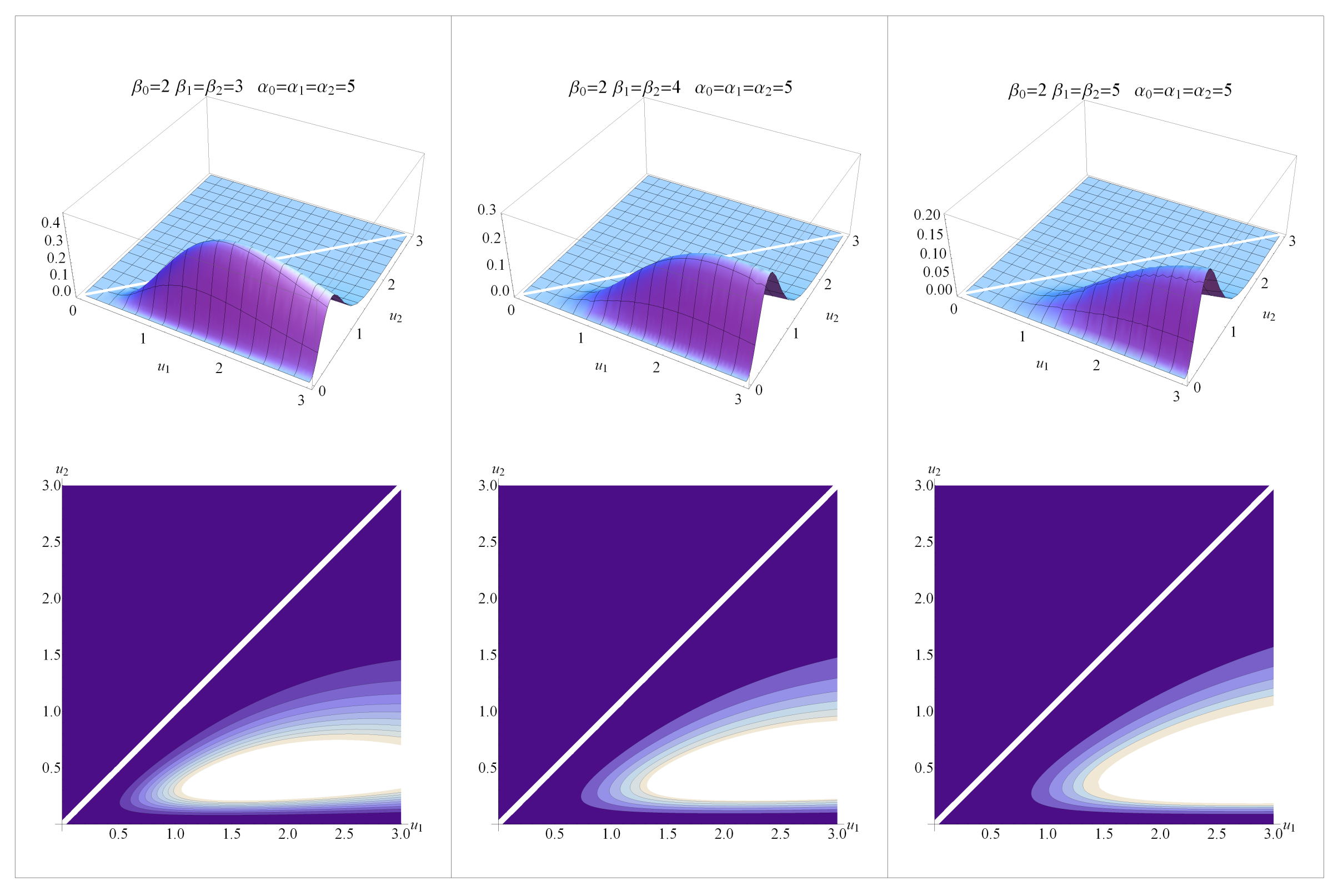
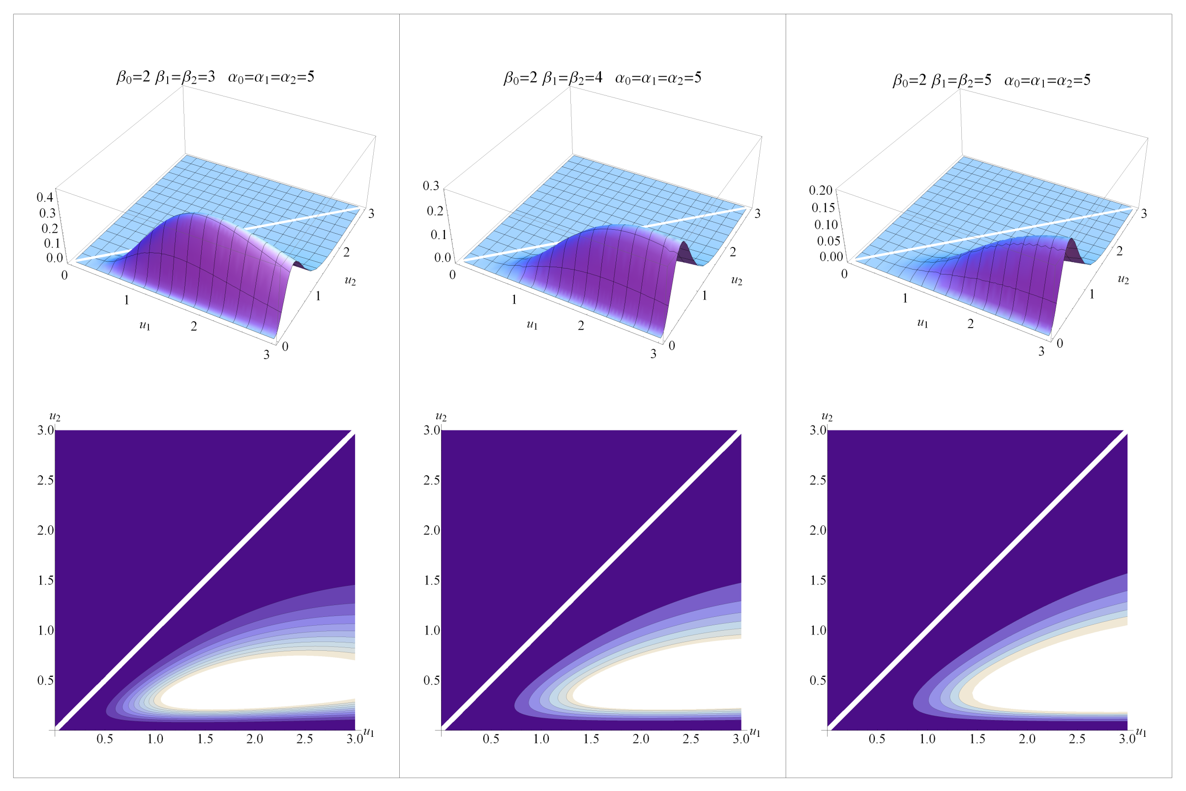
Theorem 1.
Let W i be independent gamma random variables with parameters α i = n i 1 2 > 0 , β i = 2 λ > 0 for i = 0 , 1 , 2 . Let U 1 = W 1 + W 2 W 0 and U 2 = W 2 W 0 + W 1 then the joint probability density function of U 1 and U 2 is given by
f u 1 , u 2 = β 0 α 1 + α 2 β 1 α 0 + α 2 β 2 α 0 + α 1 Γ α 0 + α 1 + α 2 Γ α 0 Γ α 1 Γ α 2 u 1 u 2 α 1 1 u 2 α 2 1 1 + u 1 α 2 1 + u 2 α 0 × β 1 β 2 1 + u 2 + β 0 β 2 u 1 u 2 + β 0 β 1 u 2 1 + u 1 α 0 α 1 α 2
where u 1 > u 2 > 0 .

2.2. Shape Analysis

In this section a shape analysis is conducted for the joint probability density function (11). A standard set of parameters has been chosen as a baseline. The parameters are chosen to be α 0 = α 1 = α 2 = 5 and β 0 = β 1 = β 2 = 2 , in other words, a process where all three samples consist of 5 × 2 + 1 = 11 observations, and where no shift has occurred in the process variance. Some of the parameters will then be varied from this baseline in order to investigate the effect that a change in the specific parameters will have on the general shape of the joint probability density function. Note that the change in some parameters will be large - so large that they lose practical realism; this is conducted to emphasise and investigate the general change in the shape, and is not meant to be an indication of the practical applications of the joint probability density function. The functions will only be plotted for u 1 [ 0 , 3 ] , u 2 [ 0 , 3 ] .
In Figure 4 it can be seen what effect increasing the sample sizes (while keeping them equal) has on the joint probability density function. It is seen that increasing the sample sizes also increases the height of the peak of the probability density function. Larger sample sizes also shrink the length and width of the “tails” of the joint probability density function. In essence, the larger the sample sizes ( n i = 11 , n i = 51 , n i = 101 ), the smaller the domain on which the function has non-trivial values.
Figure 5 below demonstrates that a sustained increase in the process variance, irrespective of size, minimally affects the general shape and location of the joint probability density function, but does affect the height of the probability density function’s peak. In the below example, the shift in the process variance occurs at time 1, and as one would hope and expect, the joint probability density function relies heavily on the value of the statistic at time 1, U 1 . A similar effect, where the joint probability density function relies heavily on the value of U 2 is seen when the shift occurs at time 2.

2.3. Marginal Probability Density Functions

Theorem 2.
Assume that U 1 , U 2 has the joint probability density function in (11), then the marginal probability density function of U 1 is given by
f u 1 = β 0 α 1 + α 2 β 1 α 0 + α 2 β 2 α 0 + α 1 Γ α 0 + α 1 + α 2 Γ α 0 Γ α 1 Γ α 2 β 1 β 2 + β 0 β 2 u 1 α 0 α 1 α 2 × ( 1 + u 1 ) α 2 k = 0 α 0 ! k ! α 0 k ! u 1 k + α 1 + α 2 1 Γ α 1 Γ k + α 2 Γ k + α 1 + α 2 × 2 F 1 α 0 + α 1 + α 2 , k + α 2 ; k + α 1 + α 2 ; u 1 β 1 β 2 β 0 β 2 + β 0 β 1 + β 0 β 1 u 1 β 1 β 2 + β 0 β 2 u 1
where u 1 > 0 , α 0 , α 1 , α 2 Z , β 1 β 2 + β 0 1 + u 1 > β 0 β 2 , u 1 β 1 β 2 β 0 β 2 + β 0 β 1 + β 0 β 1 u 1 β 1 β 2 + β 0 β 2 u 1 < 1 , and the marginal probability density function of U 2 is given by
f u 2 = β 0 α 1 + α 2 β 1 α 0 + α 2 β 2 α 0 + α 1 Γ α 0 + α 1 + α 2 Γ α 0 Γ α 2 1 + u 2 α 0 k = 0 α 2 ! k ! α 2 k ! × l = 0 1 l α 0 + α 1 + α 2 + l 1 l β 0 β 2 + β 0 β 1 u 2 α 0 α 1 α 2 l × β 1 β 2 + β 1 β 2 u 2 β 0 β 2 u 2 + β 0 β 1 u 2 l u 2 k α 0 l 1 Γ α 0 + α 2 + l k Γ α 0 + α 1 + α 2 + l k
where u 2 > 0 , α 0 , α 1 , α 2 Z , α i , β i > 0 for i = 0 , 1 , 2 and 2 F 1 , is the Gauss hypergeometric function ([6] p. 1005). Note that in (12) if α 0 1 , 2 , the sum changes from k = 0 to k = 0 α 0 (See [6] p. 25, Equations 1.110 and 1.111). Similarly if α 2 1 , 2 , the sum changes from k = 0 to k = 0 α 2 in (13).
If β 0 = β 1 = β 2 it follows that:
f u 1 = Γ α 0 + α 1 + α 2 Γ α 0 Γ α 1 Γ α 2 1 + u 1 α 0 α 1 k = 0 α 0 ! k ! α 0 k ! u 1 k + α 1 + α 2 1 × Γ α 1 Γ k + α 2 Γ k + α 1 + α 2 2 F 1 α 0 + α 1 + α 2 , k + α 2 ; k + α 1 + α 2 ; u 1
where 0 < u 1 < 1 , and
f u 2 = Γ α 0 + α 1 + α 2 Γ α 0 Γ α 2 1 + u 2 α 0 k = 0 α 2 ! k ! α 2 k ! j = 0 1 j α 0 + α 1 + α 2 + j 1 j × 1 + u 2 α 0 α 1 α 2 u 2 k α 0 j 1 Γ α 0 + α 2 + j k Γ α 0 + α 1 + α 2 + j k
where u 2 > 0 .

2.4. Product Moment and Order Statistics

Theorem 3.
Assume that U 1 , U 2 has the joint probability density function (11), then the product moment of U 1 and U 2 is given by
E U 1 r U 2 s = p = 0 r r p β 0 α 1 p s β 1 α 1 β 2 p + s Γ α 2 + p + s Γ α 0 + α 1 p s Γ α 1 + r p Γ α 0 r Γ α 0 Γ α 1 Γ α 2 Γ α 0 + α 1 p × 2 F 1 α 0 + α 1 p s , α 1 + r p ; α 0 + α 1 p ; 1 β 0 β 2 β 1 β 2
where r , s 0 , 1 , 2 , , α 0 + α 1 > r + s , α 0 > α 1 , α 0 + α 1 > p , and 1 β 0 β 2 β 1 β 2 < 1 .
The maximum order statistics are of importance in detecting whether a shift in the process variance does indeed occur, as was discussed in Section 1 and will be demonstrated in Section 3. Although a closed form expression for the maximum order statistic is not tractable in a closed form, an expression is provided that can be implemented to calculate numerical values.
Assume that U 1 , U 2 has the joint probability density function (11), then the maximum order statistic of U 1 and U 2 can be determined either by
P m a x U 1 , U 2 < z = P U 1 < z = 0 z f u 1 d u 1
when α 0 , α 1 , α 2 (since u 1 > u 2 ).

3. Comparison Study and Discussion

Deriving the order statistics of the series of statistics in (6) and (7) is a complex task since they are neither independent nor identically distributed, (see [10]). Hence values for the 95th percentiles of the maximum order statistics are simulated for varying numbers of samples (m equal to 1, 4, 9, 14, 19, 24, 29, 49, 99 and 499) and sample sizes (n equal to 2, 5, 10, 15, 20, 25, 30, 50, 100 and 500) in Section 3.1.
In Section 3.1, properties of (7) are also studied when no shift in the variance occurs, this is imperative since the control limits of a control chart are constructed under the null hypothesis that no shift has occurred, or alternatively given that the process is in control. The in control properties that are investigated for both the Q chart and the new proposed model (6) are where the maximum order statistic is most likely to occur when no shift has occurred in the process variance. Practically, this is a very important question since, if the maximum order statistic consistently occurs at roughly the same place in the sequence of samples, it implies that the distribution should be treated with added suspicion if it indicates that a shift in the process occurs at this location.
In Section 3.2, the out of control performance of the newly proposed distribution is compared with the Q chart model investigated by [5]. The probability that the respective control charts will detect a shift in the process variance is investigated for differing sizes of shifts in the process variance. The comparison is made for varying numbers of samples as well as sample sizes.

3.1. Comparison When the Process Is in Control

The location of the maximum order statistic when the process is in control is investigated using graphs. For brevity’s sake only one possible combination ( m = 29 , n = 15 ) of the number of samples and sample sizes mentioned above is included in this paper. All of them, however, lead to the same general conclusion.
As can be seen from Figure 6 the [5] distribution’s maximum order statistic occurs most often at the first statistic, with the probability of the maximum occurring at subsequent statistics steadily decreasing. This implies that the Q chart becomes more stable as the process progresses, which makes practical sense since each subsequent statistic includes more of the sample data. The newly proposed distribution’s maximum order statistic occurs most often at the first statistic, and second-most often at the last statistic. This due to the way in which the statistics of the distribution are constructed (see (6)). This implies that while our proposed model may detect shifts at the ends of the samples, signals received at these locations should be treated with a bit of skepticism.
In Table 1 the 95th percentiles of the maximum order statistics of the newly proposed distributions are simulated (to the third decimal) using Monte Carlo simulation. In other words z in the equation P m a x U 1 * , U 2 * , , U m * < z = 0.95 . Similarly the 95th percentiles of the maximum order statistics of (6) are simulated in Table 2.
Note that:
  • Since the critical values of the distribution are derived under the assumption of the null hypothesis, the equations for the maximum order statistic can be simplified to be constructed out of chi-square random variables instead of the more complex gamma case.
  • When the sample sizes of all the samples are equal n i = n for i = 1 , , m the removal of the constant terms in (7) is superfluous since the series of statistics in (6) and (7) are merely scalar multiples of each other. This can be seen in Table 1 and Table 2 where P m a x U 1 * , U 2 * , , U m * < z P m a x U 1 , U 2 , , U m < m z .
  • Instead of using simulation, the maximum order statistics in Table 2 could have been calculated using (15). Table 3 demonstrates their equivalence for the bivariate case by numerically integrating (15).

3.2. Comparisons When the Process Is out of Control

In this section, the proposed model’s potential to detect shifts in compared with that of the Q chart form investigated by [5]. The probability of signaling that a shift in the process variance has occurred depends on a few variables. In this paper, these variables are: the number of samples, the sample size of the samples, where in the process the shift in the process variance occurs, and the size of the shift. The figures in this section take all of these parameters into account.
In each of the following figures, the probability of signaling a shift in the variance is displayed as a function of the size of the shift, where the shift size λ , ranges from λ = 1 (no shift) to λ = 5 (a 500% increase in the process variance). Many different combinations of the number of samples, the sample sizes, as well as the locations of the shift were tested; however, only the graphs that illustrate key findings are included in this paper. The chosen parameters that were simulated are: number of samples m equal to 10, 20 and 30, the sample sizes n equal to 2, 5, 10 and 20, and the location of the shift in the process variance κ occurring at (roughly, due to integer sample numbers) 25%, 50% and 75% of the way through the samples.
By simulating graphs such as those in Figure 7, Figure 8 and Figure 9, certain conclusions can be reached about the properties and efficacy of the two competing models ((5) and (9)):
  • When n = 2 , irrespective of the number of samples, the newly proposed model outperforms the Q chart. There are some caveats however that should be noted:
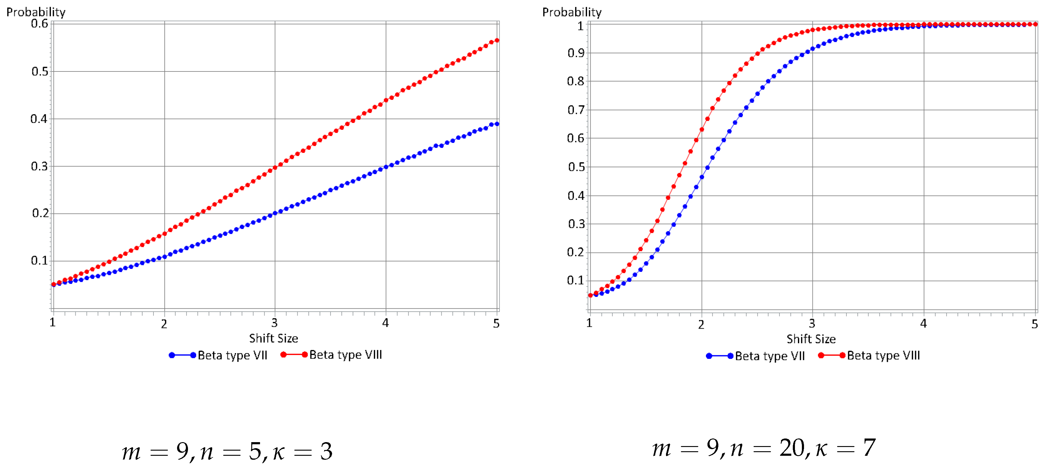
    • In the above graphs, each plotted point was simulated 500,000 times during the Monte Carlo process. For all the n = 2 graphs, the points vary erratically between each 0.05 increases in the shift size, and thus even for a large number of simulations the process cannot be described as “stable”.
    • The Q chart seems to be completely incapable of detecting an increase in the process variance when n = 2 , with the probability of detecting a shift remaining at roughly 5%, irrespective of the size of the shift.
    • While the new model’s probability of detecting a shift does increase as the size of the shift increases, it remains relatively low, at roughly 7% to 10%, just marginally higher than the 5% chance when the process is actually IC. This implies that while it might be theoretically possible to implement the new model for samples sizes of 2, it would likely not be a practically useful technique.
    • The new model’s probability of detecting a shift does not increase as the number of samples increases, as would be expected (and as is the case for the other choices of n).
  • From these points above, it can be concluded that using a sample size of 2 does not lead to an effective control chart.
  • For a small numbers of samples m = 9 , the newly proposed model outperforms the Q chart for all simulated sample sizes as well as locations of shifts (for all shift sizes).
  • When there are 20 samples m = 19 , the newly proposed model outperforms the Q chart in nearly all situations. The Q chart does have a higher probability of detecting a shift in the process variance only when the sample sizes are small n = 5 , and the shift occurs relatively late in the process κ = 15 , for shifts in the process variance between λ = 3 and λ = 4.75 . Since a 300% to 475% increase in the process variance is unlikely to occur in practice, the newly proposed model would likely be more effective for m = 19 .
  • For m = 29 , sweeping statements about the performances of the two methods are more difficult to make since the plotted percentage lines cross often. However it can be said that:
    • For small sample sizes n = 5 , the proposed model outperforms the Q chart for small shifts in the process variance, whereas the Q chart performs better for larger shifts.
    • The Q chart performs at its best when the shift in the process variance occurs late in the series of samples.
    • For larger sample sizes n = 20 the proposed model outperforms the Q chart when the shift in the process variance occurs early, but when the shift occurs roughly half way through the series of samples, or further, the performance of the two methods are very similar.

4. Concluding Remarks

In this paper a new bivariate beta type distribution is proposed that can be utilised to detect a shift in a process’s variance when the underlying process follows a normal distribution. The proposed model compares favourably with the Q chart model studied by [5] in most situations; especially when the number of samples is small, and when the process variance experiences a change early on in the series of samples. Future work can include focus on (i) when a shift occurs within a sample, (ii) expanding underlying distributional assumptions to that of the class of scale mixtures to consider departures from normality (see [11]), and (iii) the multivariate setup, of which we propose the probability density function in the following theorem and a proof outlined in the Appendix A and Appendix B.
Theorem 4.
Let W i be independent gamma random variables with parameters α i > 0 , β i > 0 for i = 0 , 1 , 2 , , m . Let U r = i = r m W i i = 0 r 1 W i , r = 1 , 2 , , m 1 , m , then the joint probability density function of U 1 , U 2 , , U m is given by
f u 1 , u 2 , , u m = i = 1 m 1 u i u i + 1 α i 1 u m α m 1 Γ i = 0 m α i i = 0 m β i α i Γ α i × 1 + u 1 i = 2 m α i i = 2 m 1 + u i α i 1 α i × 1 β 0 + u 1 u 2 β 1 1 + u 2 + i = 2 m 1 1 + u 1 u i u i + 1 β j 1 + u i 1 + u i + 1 + 1 + u 1 u m β m 1 + u m i = 0 m α i
where u 1 > u 2 > > u m > 0 .

Author Contributions

Conceptualization, S.W.H. and A.B.; methodology, S.W.H., A.B. and P.A.M.; software, P.A.M.; validation, S.W.H., A.B., J.T.F. and P.A.M.; formal analysis, P.A.M.; investigation, A.B., J.T.F. and P.A.M.; writing—original draft preparation, P.A.M.; writing—review and editing, A.B., J.T.F. and P.A.M.; supervision, S.W.H. and A.B.; funding acquisition, A.B. and J.T.F. All authors have read and agreed to the published version of the manuscript.

Funding

This work was based upon research supported in part by the National Research Foundation (NRF) of South Africa, grant RA201125576565, nr 145681; NRF ref. SRUG190308422768 nr. 120839; the RDP296/2022 grant from the University of Pretoria, South Africa, as well as the Centre of Excellence in Mathematical and Statistical Sciences, based at the University of the Witwatersrand, South Africa. The opinions expressed and conclusions arrived at are those of the authors and are not necessarily to be attributed to the NRF.

Acknowledgments

The authors acknowledge the StatDisT group based at the University of Pretoria, Pretoria, South Africa. Furthermore, the authors thank the editor as well as three anonymous reviewers for their insightful contributions which led to an improved manuscript.

Conflicts of Interest

The authors declare no conflict of interest.

Appendix A. Positioning

The aim of this section is to show the relationships between some of the most commonly used bivariate beta distributions, and to relate these distributions to the bivariate distribution derived by [5] and the one proposed by this article. In this section the statistics in the relationships are constructed out of chi-square random variables, not gamma, as is conducted throughout the rest of this article. This is conducted for the sake of simplicity; however, the relationships hold regardless.
Let Y 1 χ 2 α , Y 2 χ 2 β and Y 3 χ 2 γ . Then:
  • If Q 1 = Y 1 Y 1 + Y 2 + Y 3 and Q 2 = Y 2 Y 1 + Y 2 + Y 3 . Then the joint distribution of Q 1 and Q 2 is called a bivariate beta type I distribution. In Figure A1 this will be denoted alternatively as Q 1 , Q 2 B I α , β , γ . The multivariate generalisation of this distribution is called the Dirichlet type I distribution (see [12,13]).
  • If V 1 = X 1 X 3 and V 2 = X 2 X 3 then V 1 , V 2 has a bivariate beta type II distribution [14].
  • If W 1 = Y 1 Y 1 + Y 2 + 2 Y 3 and W 2 = Y 2 Y 1 + Y 2 + 2 Y 3 then W 1 , W 2 has a bivariate beta type III distribution. The multivariate generalisation was derived and studied by [15,16] considered the case when W 1 = Y 1 Y 1 + Y 2 + c Y 3 and W 2 = Y 2 Y 1 + Y 2 + c Y 3 , which is a generalisation of the above type III distribution.
  • If X 1 = Y 1 Y 1 + Y 3 and X 2 = Y 2 Y 2 + Y 3 then X 1 , X 2 has a bivariate beta type IV distribution, ([17,18]).
  • If C 1 = a Y 1 a Y 1 + b Y 2 + c Y 3 and C 2 = b Y 2 a Y 1 + b Y 2 + c Y 3 , a , b , c > 0 . Then C 1 , C 2 has a bivariate beta type V distribution. If a = 1 , b = 1 and c = 1 , the bivariate beta type V reduces to the bivariate beta type I [19].
  • If Z 1 = Y 1 Y 2 + Y 3 and Z 2 = Y 2 Y 1 + Y 3 then Z 1 , Z 2 has a bivariate beta type VI distribution. This joint probability density function has not yet been derived in the literature and could potentially be applied to detecting shifts in a process variance.
  • If T 1 = Y 2 Y 1 and T 2 = Y 3 Y 1 + Y 2 then T 1 , T 2 be referred to as the bivariate beta type VII distribution, ([5]).
  • If U 1 = Y 2 + Y 3 Y 1 and U 2 = Y 3 Y 1 + Y 2 then U 1 , U 2 has a bivariate beta type VIII distribution. This is the model that this article proposes in terms of gamma variables in Section 2, but in its special case it can be reduced to be constructed from chi-square variables.
Relationships between these models are graphically represented in Figure A1.
Figure A1. Relationships between several bivariate beta distributions.
Mca 27 00061 g0a1

Appendix B. Proofs

Proof of Theorem 1.
The joint probability density function of W 0 , W 1 , W 2 is given by
f w 0 , w 1 , w 2 = 1 β 0 α 0 β 1 α 1 β 2 α 2 Γ α 0 Γ α 1 Γ α 2 w 0 α 0 1 e w 0 β 0 w 1 α 1 1 e w 1 β 1 w 2 α 2 1 e w 2 β 2
where w 0 , w 1 , w 2 > 0 . Let U 0 = W 0 , then W 1 = U 0 U 1 U 2 1 + U 2 and W 2 = U 0 U 2 ( 1 + U 1 ) 1 + U 2 , and
f u 0 , u 1 , u 2 = 1 β 0 α 0 β 1 α 1 β 2 α 2 Γ α 0 Γ α 1 Γ α 2 u 1 u 2 α 1 1 u 2 α 2 1 ( 1 + u 1 ) α 2 1 + u 2 α 1 α 2 × u 0 α 0 + α 1 + α 2 1 exp u 0 β 1 β 2 1 + u 2 + β 0 β 2 u 1 u 2 + β 0 β 1 u 2 ( 1 + u 1 ) β 0 β 1 β 2 1 + u 2 .
By integrating (A2) with respect to u 0 , and rearranging the terms it follows that
f u 1 , u 2 = 1 β 0 α 0 β 1 α 1 β 2 α 2 Γ α 0 Γ α 1 Γ α 2 u 1 u 2 α 1 1 u 2 α 2 1 1 + u 1 α 2 1 + u 2 α 1 α 2 × 0 u 0 α 0 + α 1 + α 2 1 exp u 0 β 1 β 2 1 + u 2 + β 0 β 2 u 1 u 2 + β 0 β 1 u 2 ( 1 + u 1 ) β 0 β 1 β 2 1 + u 2 d u .
By applying [6] p. 346, Equation 3.381.4, to (A3), the result in (11) follows. □
Proof of Theorem 2.
From (11), by rearranging the terms, and applying [6] p. 25, Equations 1.110 and 1.111, it follows that
f u 1 = β 0 α 1 + α 2 β 1 α 0 + α 2 β 2 α 0 + α 1 Γ α 0 + α 1 + α 2 Γ α 0 Γ α 1 Γ α 2 ( 1 + u 1 ) α 2 × β 1 β 2 β 0 β 2 + β 0 β 1 + β 0 β 1 u 1 α 0 α 1 α 2 k = 0 α 0 ! k ! α 0 k ! × 0 u 1 u 1 u 2 α 1 1 u 2 k + α 2 1 β 1 β 2 + β 0 β 2 u 1 β 1 β 2 β 0 β 2 + β 0 β 1 + β 0 β 1 u 1 + u 2 α 0 α 1 α 2 d u 2 .
By applying [6] p. 317, Equation 3.197.8, to (A4), the result in (12) follows. From (11), by rearranging the terms, and applying [6] p. 25, Equations 1.110 and 1.111 twice, it follows that
f u 2 = A u 1 , u 2 u 2 u 1 u 2 α 1 1 ( 1 + u 1 ) α 2 1 + u 1 β 0 β 2 + β 0 β 1 u 2 β 1 β 2 + β 1 β 2 u 2 β 0 β 2 u 2 + β 0 β 1 u 2 α 0 α 1 α 2 d u 1 = A u 1 , u 2 k = 0 α 2 ! k ! α 2 k ! l = 0 1 l α 0 + α 1 + α 2 + l 1 l × β 0 β 2 + β 0 β 1 u 2 β 1 β 2 + β 1 β 2 u 2 β 0 β 2 u 2 + β 0 β 1 u 2 α 0 α 1 α 2 l u 2 u 1 u 2 α 1 1 u 1 k α 0 α 1 α 2 l d u 1
where
A u 1 , u 2 = β 0 α 1 + α 2 β 1 α 0 + α 2 β 2 α 0 + α 1 Γ α 0 + α 1 + α 2 Γ α 0 Γ α 1 Γ α 2 u 2 α 2 1 1 + u 2 α 0 × β 1 β 2 + β 1 β 2 u 2 β 0 β 2 u 2 + β 0 β 1 u 2 α 0 α 1 α 2 .
By applying [6] p. 315, Equation 3.191.2 to (A5), the result in (13) follows. □
Proof of Theorem 3.
By using the relationships in Figure A1, and reordering the terms it follows that
E U 1 r U 2 s = E T 1 + T 2 + T 1 T 2 r T 2 s = 0 0 t 1 + t 2 + t 1 t 2 r t 2 s g t 1 , t 2 d t 2 d t 1 = β 0 α 0 β 1 α 1 β 2 α 0 + α 1 Γ α 0 + α 1 + α 2 Γ α 0 Γ α 1 Γ α 2 0 1 + t 1 r α 0 α 1 t 1 α 1 1 × 0 t 1 1 + t 1 + t 2 r t 2 α 2 + s 1 β 1 β 2 + β 0 β 2 t 1 β 0 β 1 1 + t 1 + t 2 α 0 α 1 α 2 d t 2 d t 1 .
By applying [6] p. 25, Equations 1.110 and 1.111 to (A8), and reordering the terms, it follows that
E U 1 r U 2 s = p = 0 r r p β 0 α 0 β 1 α 1 β 2 α 0 + α 1 Γ α 0 + α 1 + α 2 Γ α 0 Γ α 1 Γ α 2 0 1 + t 1 α 0 α 1 + p t 1 α 1 + r p 1 × β 1 β 2 + β 0 β 2 t 1 β 0 β 1 1 + t 1 α 0 α 1 α 2 0 t 2 α 2 + p + s 1 1 + β 0 β 1 1 + t 1 β 1 β 2 + β 0 β 2 t 1 t 2 α 0 α 1 α 2 d t 2 d t 1 .
From [6] p. 315, Equation 3.194.3, it follows that (A8) may be expressed as
E U 1 r U 2 s = p = 0 r r p β 0 α 0 β 1 α 1 β 2 α 0 + α 1 Γ α 0 + α 1 + α 2 Γ α 0 Γ α 1 Γ α 2 0 1 + t 1 α 0 α 1 + p t 1 α 1 + r p 1 × β 1 β 2 + β 0 β 2 t 1 β 0 β 1 1 + t 1 α 0 α 1 α 2 β 0 β 1 1 + t 1 β 1 β 2 + β 0 β 2 t 1 α 2 p s × B α 2 + p + s , α 0 + α 1 + α 2 α 2 p s d t 1 = p = 0 r r p β 0 α 1 p s β 1 α 0 p s β 2 α 0 + α 1 Γ α 2 + p + s Γ α 0 + α 1 p s Γ α 0 Γ α 1 Γ α 2 × β 1 β 2 α 0 α 1 + p + s 0 1 + t 1 s t 1 α 1 + r p 1 1 + β 0 β 2 β 1 β 2 t 1 α 0 α 1 + p + s d t 1 .
By applying [6] p. 317, Equation 3.197.5 to (A9), the result in (14) follows. □
Proof of Theorem 4.
The joint probability density function of W i , i = 0 , 1 , 2 , , m is given by
f w 0 , w 1 , , w m = i = 0 m w i α i 1 e w i β i β i α i Γ α i , w 0 , w 1 , , w m > 0 .
Let U 0 = W 0 , U r = i = r m W i i = 0 r 1 W i , r = 1 , 2 , , m 1 , m . It follows that
W 0 = U 0 W 1 = U 0 U 1 U 2 1 + U 2 W r = U 0 1 + U 1 U r U r + 1 1 + U r 1 + U r + 1 , r = 2 , 3 , , m 1 W m = U 0 1 + U 1 U m 1 + U m ,
with J w 0 , , w m u 0 , u 1 , , u m = u m 1 + u 1 m 1 j = 2 m 1 + u j 2 . Subsequently the joint probability density function of U 0 , U 1 , U 2 , , U m is
f u 0 , u 1 , u 2 , , u m = i = 1 m 1 u i u i + 1 α i 1 u m α m 1 i = 0 m β i α i Γ α i u i = 0 m α i 1 1 + u 1 i = 2 m α i i = 2 m 1 + u i α i 1 α i × e u 0 1 β 0 + u 1 u 2 β 1 1 + u 2 + i = 2 m 1 1 + u 1 u i u i + 1 β i 1 + u i 1 + u i + 1 + 1 + u 1 u m β m 1 + u m .
By applying [6] p. 346, Equation 3.381.4 to (A11), the result in (16) is proved. □

References

  1. Bain, L.J.; Engelhardt, M. Introduction to Probability and Mathematical Statistics; Duxbury Press: Belmont, CA, USA, 1992; Volume 4. [Google Scholar]
  2. Pavlović, D.Č.; Sekulović, N.M.; Milovanović, G.V.; Panajotović, A.S.; Stefanović, M.Č.; Popović, Z.J. Statistics for ratios of Rayleigh, Rician, Nakagami-, and Weibull distributed random variables. Math. Probl. Eng. 2013, 2013, 252804. [Google Scholar] [CrossRef] [PubMed] [Green Version]
  3. Bilankulu, V.; Bekker, A.; Marques, F. The ratio of independent generalized gamma random variables with applications. Comput. Math. Methods 2021, 3, e1061. [Google Scholar] [CrossRef] [Green Version]
  4. Leonardo, E.J.; da Costa, D.B.; Dias, U.S.; Yacoub, M.D. The ratio of independent arbitrary α-μ random variables and its application in the capacity analysis of spectrum sharing systems. IEEE Commun. Lett. 2012, 16, 1776–1779. [Google Scholar] [CrossRef]
  5. Adamski, K. Generalised Beta Type II Distributions-Emanating from a Sequential Process. Ph.D. Thesis, University of Pretoria, Pretoria, South Africa, 2013. [Google Scholar]
  6. Gradshteyn, I.S.; Ryzhik, I.M. Table of Integrals, Series, and Products; Academic Press: Cambridge, MA, USA, 2014. [Google Scholar]
  7. Adamski, K.; Human, S.W.; Bekker, A. A generalized multivariate beta distribution: Control charting when the measurements are from an exponential distribution. Stat. Pap. 2012, 53, 1045–1064. [Google Scholar] [CrossRef]
  8. Quesenberry, C.P. SPC Q charts for start-up processes and short or long runs. J. Qual. Technol. 1991, 23, 213–224. [Google Scholar] [CrossRef]
  9. Bekker, A.; Ferreira, J.T.; Human, S.W.; Adamski, K. Capturing a Change in the Covariance Structure of a Multivariate Process. Symmetry 2022, 14, 156. [Google Scholar] [CrossRef]
  10. David, H.A.; Nagaraja, H.N. Order Statistics; John Wiley & Sons: Hoboken, NJ, USA, 2004. [Google Scholar]
  11. Ferreira, J.T.; Bekker, A.; Marques, F.; Laidlaw, M. An enriched α-μ model as fading candidate. Math. Probl. Eng. 2020, 2020, 5879413. [Google Scholar] [CrossRef] [Green Version]
  12. Gupta, R.D.; Richards, D.S.P. The history of the Dirichlet and Liouville distributions. Int. Stat. Rev. 2001, 69, 433–446. [Google Scholar] [CrossRef]
  13. Balakrishnan, N.; Lai, C.D. Continuous Bivariate Distributions; Springer Science & Business Media: Berlin/Heidelberg, Germany, 2009. [Google Scholar]
  14. Tiao, G.G.; Cuttman, I. The inverted Dirichlet distribution with applications. J. Am. Stat. Assoc. 1965, 60, 793–805. [Google Scholar] [CrossRef]
  15. Cardeno, L.; Nagar, D.K.; Sánchez, L.E. Beta type 3 distribution and its multivariate generalization. Tamsui Oxf. J. Math. Sci. 2005, 21, 225–242. [Google Scholar]
  16. Ehlers, R. Bimatrix Variate Distributions of Wishart Ratios with Application. Ph.D. Thesis, University of Pretoria, Pretoria, South Africa, 2011. [Google Scholar]
  17. Jones, M. Multivariate t and beta distributions associated with the multivariate F distribution. Metrika 2002, 54, 215–231. [Google Scholar] [CrossRef]
  18. Olkin, I.; Liu, R. A bivariate beta distribution. Stat. Probab. Lett. 2003, 62, 407–412. [Google Scholar] [CrossRef]
  19. Ehlers, R.; Bekker, A.; Roux, J.J. Triply noncentral bivariate beta type V distribution. S. Afr. Stat. J. 2012, 46, 221–246. [Google Scholar]
Figure 1. Process shift.
Mca 27 00061 g001
Figure 2. Building blocks of new distribution.
Mca 27 00061 g002
Figure 3. Building blocks of [7].
Mca 27 00061 g003
Figure 4. Equal sample sizes, no shift in the variance.
Mca 27 00061 g004
Figure 5. Equal sample sizes, increase in variance at time 1.
Mca 27 00061 g005
Figure 6. Location of maximum order statistics: m = 29 and n = 15 .
Mca 27 00061 g006
Figure 7. Probability of detecting a shift when n = 2 .
Mca 27 00061 g007
Figure 8. Probability of detecting a shift when m = 9 .
Mca 27 00061 g008
Figure 9. Probability of detecting a shift when κ 0.75 m.
Mca 27 00061 g009
Table 1. 95th percentiles of the maximum order statistics of U 1 * , U 2 * , , U m * .
mn25101520253050100500
1214.2866.6523.2302.5122.1891.9981.8721.6151.3991.160
4242.0466.2293.0472.3852.0931.9191.8051.5691.3711.150
9254.5925.9922.9082.3012.0231.8631.7551.5341.3491.142
14251.7475.8742.8712.2661.9971.8421.7391.5221.3411.139
19255.4135.8362.8512.2541.9871.8311.7301.5171.3371.137
24257.8805.8132.8372.2431.9801.8271.7231.5141.3351.137
29259.1055.8152.8242.2381.9771.8221.7201.5121.3341.136
49259.9635.7992.8182.2281.9681.8151.7151.5081.3311.135
99258.8105.7972.8032.2221.9591.8111.7101.5041.3291.134
499263.0175.7722.8012.2151.9571.8081.7071.5011.3281.133
Table 2. 95th percentiles of the maximum order statistics of U 1 , U 2 , , U m .
mn25101520253050100500
1399.76212.0915.9334.6384.0723.7353.5133.0622.6882.275
41151.10329.01514.06111.0459.7088.9588.4347.4116.5535.618
92413.47057.22227.64921.69919.10117.62316.61514.61512.98411.184
143691.86185.49641.14432.37628.46926.29224.83721.86419.41916.754
194944.966112.74454.65643.07137.87034.91333.02029.08125.81622.318
246187.147141.31568.32553.65347.31343.54941.18236.29332.24827.887
297528.303170.17481.75364.40856.62152.31349.39743.53138.67833.457
4912,560.904281.708135.824107.16394.20086.90082.16872.39564.34955.728
9925,774.144565.834270.688213.065187.991173.740164.160144.638128.625111.365
499126,434.2462815.1861353.4581064.841939.259868.035819.248722.038642.752556.808
Table 3. Simulated and theoretical 95th percentiles of the maximum order statistics of U 1 , U 2 .
Methodn25101520253050100500
Simulated values399.76212.0915.9334.6384.0723.7353.5133.0622.6882.275
Theoretical values399.00012.0835.9204.6404.0683.7353.5153.0642.6882.276
Publisher’s Note: MDPI stays neutral with regard to jurisdictional claims in published maps and institutional affiliations.

