Learning Motion Primitives Automata for Autonomous Driving Applications

Abstract

Motion planning methods often rely on libraries of primitives. The selection of primitives is then crucial for assuring feasible solutions and good performance within the motion planner. In the literature, the library is usually designed by either learning from demonstration, relying entirely on data, or by model-based approaches, with the advantage of exploiting the dynamical system’s property, e.g., symmetries. In this work, we propose a method combining data with a dynamical model to optimally select primitives. The library is designed based on primitives with highest occurrences within the data set, while Lie group symmetries from a model are analysed in the available data to allow for structure-exploiting primitives. We illustrate our technique in an autonomous driving application. Primitives are identified based on data from human driving, with the freedom to build libraries of different sizes as a parameter of choice. We also compare the extracted library with a custom selection of primitives regarding the performance of obtained solutions for a street layout based on a real-world scenario.

1. Introduction

In engineering, modern computational tools for simulation, optimization, and control have become inevitable, starting from early in the design phase up to the operation of the systems. These numerical methods strongly rely on dynamical system models, and thus, their performance is directly restricted by the model accuracy. Two approaches can be followed for defining dynamical system models: using physics-based model equations with a suitable tuned (small) set of parameters or data-based models of generic structure with a (large) set of parameters to be learned from data in an automated way. While these approaches have formerly been considered diametrically opposed, in recent years, more and more fruitful combinations from both worlds have been proposed. In particular, the term physics-inspired learning has been coined for methods that integrate physical knowledge in data-based modeling techniques [1,2,3].

In this contribution, we propose a physics-based learning approach based on motion primitives (MP). It results in a maneuver automaton (MA), which can be used for efficient trajectory planning, e.g., in autonomous driving applications. The primitives are characterized as short snippets of solutions: given a dynamical system with symmetries, MP are equivalence classes of controlled maneuvers. In particular, constantly controlled relative equilibria are called trim primitives.

For motion planning with MP, the selection of a primitives’ library is of fundamental importance for the feasibility and the performance quality of the planning. Procedures presented in the literature include a custom selection based on possible operating points [4,5], which can include maneuvers by optimal control methods [6,7,8], numerical approximation from a simplified state machine of actions [9], and extraction from experts’ driving trajectories [10,11]. As an expansion of the library, Ref. [12] propose an exploration phase via reinforcement learning and, then, extracting and adding new trims and maneuvers to the initial library.

Yet, MP bridge the model perspective and the data viewpoint: considering a human controlling a technological system and partial solutions to control problems, i.e., primitives, which have been learned (probably subconsciously) are repetitively used and which can be concatenated by the operator according to the current situation [6]. Based on data from human driving, we identify MP and construct a MA, which is then fed to a trajectory planner for autonomous vehicles.

1.1. Related Work

As detailed in the following, so far, a library has alternatively been comprised of data-based or of model-based primitives, exclusively. For data-based primitives, one aims to solve the learning from demonstration problem, in which, based on an expert’s solution, a policy mapping the states to inputs is adjusted. In the model-based approach, the dynamical system is represented by an ordinary differential equation, and the MP can be extracted by mathematical analysis.

According to [13], there are two methods for learning from demonstration: (1) the mimic of the MP using some dynamical system, for example, dynamic motion primitives (DMP) [14,15] and applications of inverse optimal control [16]; and (2) statistical machine learning methods, such as hidden Markov models [17], Gaussian mixture models [18], probabilistic motion primitives [19], and kernelized movement primitives [20] with its extensions [21]. These methods are suitable for repetitive tasks of typical scenes. However, they do not take into consideration a dynamical system model, making it difficult to develop mathematical analysis of, for example, robustness or stability assurance. The generalization of the motions is totally reliant on the machine learning algorithm and the sample data characteristics. In particular, DMP are shown to have the advantage of better generalization, being able to adapt for the motion planning specifications and to be robust to perturbations [22]. This method extracts the motion features by adjusting the parameters of basis functions, being able to learn the positions, velocities and acceleration time-wise. It is used in a wide range of applications from robotics to biological control [23].

In this regard, the work from [11] stands out. It proposes a segmented representation, extraction, and library establishment of MP. They achieved it by a modified DMP method for representation, implementing a probabilistic extraction algorithm for the segmentation of the unlabeled trajectory data and connecting the MP by correlating the representation parameters. However, as disadvantages, it showed a lower accuracy in the representation at the end of each MP, affecting the connection transition over them and the inability to design emergency driving behaviour. Also, studying an extension of DMP, [24] concluded that it is hard for the DMP to ensure kinodynamic feasibility.

On the other hand, there are the model-based approaches to select MP. As one of the simplest cases, there are Dubins curves [25]. Here, three possible MP apply a constant action over an interval of time: turn left or turn right and go straight. Dubins considers a simple kinematic car model, consisting only in the pose, i.e., the position and orientation. Reeds–Shepp curves are a natural extension of Dubins’ work by also allowing traveling in the reverse direction [26].

It is also possible to exploit some properties of the system to design the MP. In [6], the invariance property was exploited to generate two types of MP: trim primitives and maneuvers. The first ones are relative equilibria under constant control, while the second are controlled trajectories starting and ending on trims. Then, a MA is generated in the form of a directed graph. Here, trims are represented by vertices and maneuvers by edges of the graph, such that a graph-based planning method can determine admissible or optimal sequences of MP which form a trajectory plan.

Since the approach is based on a continuous-time dynamical model, in principle, it would be possible to generate a large amount of primitives. Although more MP could improve the planner’s performance in practice, it can also increase the difficulty of ensuring resolution completeness [27]. The number of MP is thus an important design parameter of the planning method. It should be noted that the importance of MP, especially in the field of autonomous driving, was showed in different applications, e.g., in motion planning [6], in driving style recognition [28], and to predict drivers’ behaviours [29].

With a MA ruling the concatenation of primitives, the motion planning problem becomes the search for the best sequence of MP that lead to a goal state. This can be accomplished through graph-search algorithms, for instance A*, which is today presumably the most well-known best-first search algorithm [30,31,32]. The characteristic of A* is the expansion of nodes based on an evaluation function, which is a sum of two costs: 1) from the start point to the considered node and 2) from the node to the goal [32]. While A* deals with fully discrete states, e.g., centers of grid-cells when applied to a continuous state space, the Hybrid A* is more suitable for MP of dynamical systems as it associates the cost of continuous state trajectories to grid-cells [33,34]. As an alternative, the authors presented the Optimized Primitives (∏*) algorithm in a previous work [4]. It admits any continuous point in the state space, without associations to grid-cells. In addition, it solves an optimization problem of reduced complexity to adjust the duration of trim primitives to let the vehicle reach any desired point in the state space, e.g., an exact goal pose. An alternative method suitable for multi-agent systems is to deal with the graph search as a receding horizon problem [35].

1.2. Contributions

In this paper, we propose a novel grey-box method combining data-based learning with model-based automata. We use the differential geometric description of relative equilibria to reveal Lie group symmetries and invariances in data and present the symmetry group for a generic class of vehicle models. An automaton can be designed which is tailored to include primitives which have the highest occurrences within the data. Here, we use data from human driving in real-world traffic scenarios and street layouts. In the analysis, we focus on the representation of trajectories mimicking the human-driven solutions within the automaton. The resulting data-based automaton is shown to outperform handcrafted automata of comparable size, but based on model information only, in planning tests. Thus, we propose modeling techniques which allow reliable but efficient trajectory planning as needed for autonomous driving.

2. Dynamical Control System Representation by Automata

Our starting point will be an autonomous dynamical system with control, $\dot{x}=f(x,u)$ on an n-dimensional state manifold $\mathcal{X}$ and an m-dimensional control space $\mathcal{U}\subset {\mathbb{R}}^m$. We consider trajectory planning problems in the form:

$$\begin{array}{c}\hfill \begin{array}{cc}\hfill \mathrm{Find}& (x,u):[0,T]\to \mathcal{X}\times \mathcal{U}\mathrm{and}T\in {\mathbb{R}}^{+},\hfill \\ \hfill \mathrm{such}\mathrm{that}& \dot{x}=f(x,u)\mathrm{and}\hfill \\ \hfill & g\left(x\right(t),u(t\left)\right)\le 0\forall t\in [0,T],\hfill \\ \hfill & x\left(0\right)=x_0,x\left(T\right)=x_T.\hfill \end{array}\end{array}$$

(1)

Later on, we add an optimization criterion $J(x,u)={\int }_0^T\ell (x\left(t\right),u\left(t\right))dt+\mu \left(x\left(T\right)\right)$ to obtain an optimal control problem constrained by (1). Let us assume the existence of unique solutions for suitable chosen inputs u on the time interval $[0,T]$ being ensured, such that x on $[0,T]$ is given by the flow, $x\left(t\right)={\phi }_u(x_0,t)$ with $x\left(0\right)=x_0$.

In general, nonlinear, complex dynamical models pose difficulties to numerical optimization techniques, e.g., in optimization-based real-time control schemes such as model predictive control (MPC). Thus, simplified system models ranging from equivalent system reformulations up to scalable system approximations are of interest from the application point of view. For instance, the motion primitive approach of Frazzoli et al. [6] combines an exact reformulation in terms of MP with a discrete approximation of system dynamics in terms of an automaton.

2.1. Symmetry and Motion Primitives

We focus on dynamical systems with symmetries which act as state transformations defined by Lie group representations. Excluding finite Lie groups (used for modeling permutations, reflections, or rotations by fixed angles), we consider continuous Lie groups of compact and non-compact form, as they model, e.g., rotations, translations, and combinations thereof [36]. Let the Lie group be denoted by $\mathcal{G}$, its identity element by e, and its left action on $\mathcal{X}$ by $\Psi :\mathcal{G}\times \mathcal{X}\to \mathcal{X}$ with $\Psi$ smooth, $\Psi (e,x)=x$ for $x\in \mathcal{X}$, and $\Psi (g,\Psi (h,x\left)\right)=\Psi (gh,x)$ for all $g,h\in \mathcal{G}$ and $x\in \mathcal{X}$.

Definition 1

(Symmetry). The tupel $(\mathcal{G},\Psi )$ is a symmetry for $\dot{x}=f(x,u)$ on $\mathcal{X}$, if for any fixed control $u\in {\mathcal{L}}_{\mathrm{loc}}^{\infty }([0,\infty ),{\mathbb{R}}^m)$, it holds for all $g\in \mathcal{G}$, $x\in \mathcal{X}$, and $t\ge 0$,

$${\phi }_u(\Psi (g,x_0),t)=\Psi (g,{\phi }_u(x_0,t)).$$

(2)

Remark 1.

Equivalently, we could ask for

• $(\mathcal{G},\Psi )$ to generate trajectories, i.e., for any given trajectory x on $[0,T]$, $T>0$, with corresponding control u on that time interval, also $(\Psi (g,x),u)$ satisfies the dynamical system equations, i.e., it is a solution for any group element $g\in \mathcal{G}$;
• the vector field being equivariant w.r.t. $(\mathcal{G},\Psi )$, i.e.,

  $$f(\Psi (g,x),u)={\Psi }^{T\mathcal{X}}(g,f(x,u))$$

  (3)

  for any pair $(x,u)\in \mathcal{X}\times \mathcal{U}$ and ${\Psi }^{T\mathcal{X}}$ being the lift of the symmetry action (detailed out e.g., in [8]);
• the invariance of the Lagrangian or the Hamiltonian w.r.t. $(\mathcal{G},\Psi )$, if we have a mechanical system of this kind [7,37,38,39].

In any case, symmetry allows us to reduce the set of all admissible pairs $(x,u)$ via the equivalence relation based on the symmetry action.

Definition 2

(Motion Primitive). A motion primitive is the equivalence class of a representing pair $(x,u)$ on $[t_i,t_f]$, if for any class member $(\overline{x},\overline{u})$ on $[{\overline{t}}_i,{\overline{t}}_f]$, $t_f-t_i={\overline{t}}_f-{\overline{t}}_i$ and there exists a group element $g\in \mathcal{G}$ and a shift $\Delta t\in \mathbb{R}$, such that

$$(x\left(t\right),u\left(t\right))=(\Psi (g,\overline{x}(t-\Delta t)),\overline{u}(t-\Delta t))\forall t\in [t_i,t_f].$$

By slight abuse of notation, we also call the representative $(x,u)$ a motion primitive. The set of MP is denoted by $\mathcal{P}$.

2.2. Trim Primitives

The name trim primitives has been introduced in [6], since these MP are characterized by fixed, i.e., trimmed, controls. Moreover, they are symmetry-induced motions.

Definition 3

(Trim Primitive). Based on the setting of Definition 1, let $\mathfrak{g}$ denote the Lie algebra of $\mathcal{G}$ and $exp:\mathfrak{g}\to \mathcal{G}$ the exponential map. Let $\overline{u}\in \mathcal{U}$. The tupel $(x,u)$ on $[0,T]$ with $x\left(0\right)=x_0$ is called a trim primitive if it is a solution to the system dynamics which can be expressed by

$$x\left(t\right)=\Psi (exp\left(\xi t\right),x_0),u\left(t\right)\equiv \overline{u},\forall t\in [0,T],$$

(4)

with $\xi \in \mathfrak{g}$ being a suitable chosen Lie algebra element.

We refer to, e.g., [37] for the following definitions, also summarized in [39]. The Lie algebra is defined as the vector space $T_e\mathcal{G}$, and it is isomorphic to the vector space of left-invariant vector fields on $\mathcal{G}$. That is, for $\xi \in \mathfrak{g}$, there is a vector field $X_{\xi }$, such that a solution ${\gamma }_{\xi }:\mathbb{R}\to \mathcal{G}$ of ${\gamma }_{\xi }^{\prime }\left(t\right)=X_{\xi }\left({\gamma }_{\xi }\left(t\right)\right)$ with ${\gamma }_{\xi }\left(0\right)=e$ is a one-parameter subgroup in $\mathcal{G}$. The exponential map $exp:\mathfrak{g}\to \mathcal{G}$ is defined by $exp\left(1\right)={\gamma }_{\xi }\left(1\right)$. Then, a line $t\xi$ in $\mathfrak{g}$ for $t\in \mathbb{R}$ is mapped via $exp\left(t\xi \right)={\gamma }_{\xi }\left(t\right)$ to a one-parameter subgroup in $\mathcal{G}$. Furthermore, the orbit of x is defined by $\mathrm{Orb}\left(x\right)=\{\Psi (g,x\left)\right|g\in \mathcal{G}\}\subset \mathcal{X}$.

Fixing the control to a constant value $\overline{u}\in \mathcal{U}$ allows us to study the $\overline{u}$-parametrized vector field $f_{\overline{u}}\left(x\left(t\right)\right)$: trim primitives are relative equilibria of $\dot{x}\left(t\right)=f_{\overline{u}}\left(x\left(t\right)\right)$, i.e., $x_{\mathrm{tr}}$ belongs to a relative equilibrium if the vector field $f_{\overline{u}}:\mathcal{X}\to T\mathcal{X}$ points in the direction of the group orbit $\mathrm{Orb}\left(x_{\mathrm{tr}}\right)$ through $x_{\mathrm{tr}}$, i.e.,

$$f_{\overline{u}}\left(x_{\mathrm{tr}}\right)\in T_{x_{\mathrm{tr}}}\left(\mathrm{Orb}\left(x_{\mathrm{tr}}\right)\right).$$

(5)

Equivalently, $x_{\mathrm{tr}}$ belongs to a relative equilibrium if there exists $\xi \in \mathfrak{g}$ such that, with the group orbit $g\left(t\right):=exp\left(\xi t\right)$, we have $x\left(t\right)=\Psi (exp\left(\xi t\right),x_{\mathrm{tr}})$ as a solution for the dynamics. In [38], the alternative definitions are discussed in detail for Hamiltonian mechanics.

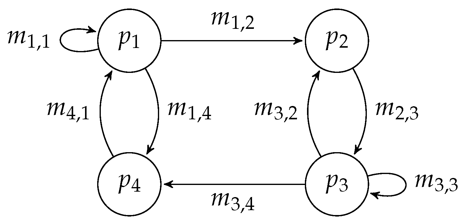
2.3. Automaton and Sequencing

Maneuvers are MP, i.e., controlled trajectories on some fixed time-interval $[0,T]$, which allow us to link trim primitives.

Definition 4

(Maneuver). A motion primitive is called a maneuver if it connects two trim primitives, i.e.,  applying suitable symmetry shifts and time shifts, the sequence trim–maneuver–trim generates a trajectory which is admissible to the system dynamics.

The trajectory planning problem on $\mathcal{X}\times \mathcal{U}$ could equivalently be posed on the set of MP thanks to the symmetry property. However, to generate a system representation by a finite automaton, a finite number of MP need to be chosen. Choose a finite set of MP $(P,M)\subset \mathcal{P}$, divided into trim primitives P and maneuvers M. Let P define the vertices of a graph to define the MP automaton. An edge $m_{i,j}$ is included in the automaton if trim $p_i\in P$ and trim $p_j\in P$ are connected by a maneuver in M, which is then denoted by $m_{i,j}$, as illustrated in Figure 1.

Then, we have the following property.

Proposition 1.

Consider the trajectory planning problem (1). If there are initial and final trims $p_0,p_T\in P$ such that $x_0\in p_0$ and $x_T\in p_T$ and if there exists a path within the automaton connecting $p_0$ to $p_T$, then a trajectory-control-pair can be generated which is admissible to problem (1).

Formal details on the concatenating of MP based on automaton sequences and on the reconstructing of corresponding trajectories are given in [6]. They form a constructive proof to the statement above.

As discussed in Section 1.1, various graph-based search methods can be applied for finding admissible or optimal sequences of trajectories. We refer to the cited literature without giving further details, since this paper is not focused on the planning, but on the modeling aspect, i.e., on the optimal generation of automata.

2.4. Shortcomings

The motion planning by MP approach has been extended by Frazzoli and his cofounders, as well as by several others, see, e.g., [5,6,7,12,40,41,42]. However, some issues remain: first, the MP are specific to a certain system, e.g., a specific vehicle, since they typically depend on parameters. Thus, the automaton has to be adapted to each individual system. Second, as previously mentioned, the size of automaton is crucial: a larger automaton provides a better representation of the original control system behaviour, but the search within planning algorithms can become computationally more costly. Thus, finding an optimal trade-off is desirable and can be based on the following criteria. The Lie algebra contains all candidate elements to generate trim primitives. It is reasonable to generate a set of trims via gridding the Lie algebra [42]. However, the choice of trims, i.e., the size of the Lie algebra grid and the total amount of trims are up the designer. Moreover, the number of maneuvers and which trims to directly link via a maneuver is up to design as well: a high number of maneuvers might improve reachability within the graph and allows for optimizing among admissible sequences. Again, this comes at the cost of higher computation times. Ideally, one would like to restrict to needed maneuvers a priori to solve or even know the posed trajectory planning problems.

While the first issue of individualized automata for each different vehicle would have to be resolved via parameter identification, which is beyond the focus of this paper, the latter issue with all its subproblems is addressed in the following sections by including data to the modeling procedure. Thus, the overall aim is to design an automaton capable of representing realistic dynamical behaviour.

3. Generating Data-Based Automata

In this section, we describe our approach for generating motion primitive automata, as introduced in Section 2, based on data of a dynamical system in general. We assume a basic dynamical model to be known, as well as its symmetries, such that we can focus on the following steps:

1.

Finding invariances in terms of trims in data,

2.

Clustering trim primitives,

3.

Evaluating a transition matrix,

4.

Computing maneuvers.

We discuss these steps in detail in the following.

3.1. Assumptions on Data and Model

We assume data in terms of sets of triples $(t^k,y^k,u^k)$ consisting of (partial) state observations, with time stamps, augmented by the applied control input sequence, i.e.,

$$\mathbb{D}=\bigcup _{k=0}^D(t^k,y^k,u^k)$$

such that, for all sets, $k=0,\cdots ,D$, we have $(t^k,y^k,u^k)=((t_0^k,y_0^k,u_0^k),\cdots ,(t_{N_k}^k,y_{N_k}^k,u_{N_k}^k))$ with time points satisfying $t_0^k<t_1^k<\cdots <t_{N_k}^k$ and a minimum length of two, $N_k\ge 1$.

Based on a priori knowledge on the observed system, a continuous-time model $\dot{x}=f(x,u)$ needs to be chosen as introduced in Section 2, together with sets of admissible states and controls. That is, the choice of control space $\mathcal{U}$ has to satisfy $u_j^k\in \mathcal{U}$ for $0\le j\le N_k$ and $0\le k\le D$. Furthermore, the state space $\mathcal{X}$ has to be chosen with $\mathcal{Y}\subseteq \mathcal{X}$ and $y_j^k\in \mathcal{Y}$ for $0\le j\le N_k$ and $0\le k\le D$. In general, it might hold that $dim\left(\mathcal{Y}\right)<dim\left(\mathcal{X}\right)$, because rarely are there sensors available measuring every internal state of a dynamical system model. However, control theory provides the method for observers to reconstruct missing states. Since observer design is not within the scope of this paper, let us assume the model is observable such that the full system state could be reconstructed. To simplify notation, we drop $\mathcal{Y}$ and rename the data as

$$\mathbb{D}=\bigcup _{k=0}^D(t^k,x^k,u^k)\mathrm{with}(t^k,x^k,u^k)={\left\{(t_j^k,x_j^k,u_j^k)\right\}}_{j=0}^{N_k}$$

and $x_j^k\in \mathcal{X}$ for all $0\le j\le N_k$ and $0\le k\le D$.

Finally, the model $\dot{x}=f(x,u)$ has to possess trims as introduced in Section 2, i.e., based on a suitable chosen symmetry $(\mathcal{G},\Psi )$, there exist solutions $(x,u)$ satisfying Definition 3. Despite assuming the symmetry group $\mathcal{G}$, its action $\Psi$, and the corresponding Lie algebra $\mathfrak{g}$ to be given, these can only be thought of as the maximal set of trim primitives which might exist within the recorded data.

3.2. Identifying Trim Primitives in Data

We now aim to identify data points which belong to trim primitives. Recall from Definition 3 that model-based trims are defined as trajectories being expressed via $x\left(t\right)=\Psi (exp\left(\xi t\right),x_0)$, $u\left(t\right)\equiv \overline{u},\forall t\in [0,T]$. Pick a one-dimensional group orbit $g\left(t\right):=exp\left(\xi t\right)$ for $t\in [0,T]$. If $x_{\mathrm{tr}}$ is the initial point ($x_0$ in Definition 3) of a trim with corresponding $\xi \in \mathfrak{g}$, then all

$$x\in {\mathrm{Orb}}_{\xi }\left(x_{\mathrm{tr}}\right):=\{\Psi (g\left(t\right),x_{\mathrm{tr}})|g\left(t\right)=exp\left(\xi t\right),t\in [0,T]\}$$

belong to the same trim. Since a trim is a motion primitive (see Definition 2), the requirement $x_{\mathrm{tr}}=x_0$ can be relaxed by introducing suitable time shifts. Moreover, all $x\in {\mathrm{Orb}}_{\xi }\left(x_{\mathrm{tr}}\right)$ share the property that, cf. Equation (5), $f_{\overline{u}}\left(x\right)\in T_x\left({\mathrm{Orb}}_{\xi }\left(x_{\mathrm{tr}}\right)\right)$, which can be used for identifying trims.

Remark 2

(Systems with Cyclic Variables). The most obvious way in which a symmetry of $\dot{x}=f(x,u)$ may occur is via independence w.r.t. some of the states. In geometric mechanics, these (configuration) states are called cyclic [38]. In fact, the configuration manifold Q is split into the shape space S and multiple copies of $S^1$ (for rotational symmetry) or $\mathbb{R}$ (for translational symmetry, respectively), i.e., $Q=S\times S^1\times \dots \times S^1$ and $\mathcal{X}=TQ$. Symmetry action Ψ is then restricted to be the identity on S, and thus, the coordinates in S are necessarily constant along a trim primitive. In this case, this provides a characteristic for automatically detecting trim primitives in data.

The vehicle models we consider in Section 4.2 do not only have cyclic variables though, but a subgroup of $SE\left(3\right)$ as their symmetry group.

For now, we have to analyze each data set $(t^k,x^k,u^k)\in \mathbb{D}$ separately. Thus, let us omit index k for the time being. Identical trims across different sets will be found subsequently by a clustering method as described in Section 3.3.

Corollary 1.

As it follows directly from Definition 3 for all ${\left\{(t_j,x_j,u_j)\right\}}_{j=t_i}^{t_e}$ with $0\le t_i,t_e\le N$ belonging to the same trim, necessarily, it holds that there is a $u_t\in \mathcal{U}$ and ${ϵ}_u>0$ small, such that $\left|\right|u_j-u_t\left|\right|<{ϵ}_u$ for $t_i\le j\le t_e$.

While there are examples of control systems in which every constant control input generates a trim primitive, e.g., the holonomic robot/kinematic car as studied in [8], this property is not sufficient, in general.

Corollary 2.

Assuming $\left|\right|u_{i+1}-u_i\left|\right|<ϵ$ as in Corollary 1. Then, the corresponding data points belong to a trim if there exists $\xi \in \mathfrak{g}$ and ${ϵ}_x>0$ small, such that

$$\left|\right|\Psi (exp\left(\xi (t_{i+1}-t_i)\right),x_i)-x_{i+1}\left|\right|<{ϵ}_x.$$

In the most general setting, the Lie algebra element $\xi$ could be found by a regression problem. A threshold on the fitting error would then be used to decide whether a sequence of points is a trim. However, $\xi$ can often be directly linked to the velocities within a system, as it is shown for the vehicle models studied in Section 4. This simplifies the classification step. The choice of ${ϵ}_x$ is crucial but problem-dependent, since it has to be balanced against the noise within the data, which itself might split up trims in a too sensitive scanning. Finally, let us remark that classification based on thresholds, i.e., rectangular decision boundaries, is not the only choice, see e.g., quadratic discriminant analysis based on probability computations, e.g., [43].

3.3. Clustering Trim Primitives

Let all identified trim primitives be collected in P. For $i=1,\cdots ,\left|P\right|$, let $p_i\in {\mathbb{R}}^p$ denote the defining values of the trim, e.g., the generating Lie algebra element, the constant control value, and $x_0:=x_{t_i}$ in the notation of Corollary 1. We now aim at finding trims, also from different trajectories, which are similar. More precisely, we look for a finite amount of clusters of trims and define a single representative trim for each cluster.

We choose to work with the k-means algorithm, an unsupervised learning technique to find clusters in a set of data points [44]. Fixing the number of clusters to $n_{\sigma }$, the k-means algorithm finds the clusters $C_1,\dots ,C_{n_{\sigma }}\subset P$, with ${\bigcup }_{j=1}^{n_{\sigma }}{C}_j=P$, and representative trims ${\sigma }_j,j=1,\dots ,n_{\sigma }$, in which ${\sigma }_j\in {\mathbb{R}}^p$ is the center of the $j^{\mathrm{th}}$ cluster in ${\mathbb{R}}^p$. This is accomplished by minimizing the following objective function (also called as distortion measure) [45]:

$$J_P=\sum _{i=1}^{\left|P\right|}\sum _{j=1}^{n_{\sigma }}{\alpha }_{ij}\left|\right|p_i-{\sigma }_j{\left|\right|}^2$$

(6)

where ${\alpha }_{ij}\in \{0,1\}$ is a binary indicator variable, defining to which cluster the trim $p_i$ is assigned. There is a two-stage optimization process: First, $J_P$ is minimized w.r.t. ${\alpha }_{ij}$, keeping initial values of ${\sigma }_j$ fixed. Then, $J_P$ is minimized w.r.t. ${\sigma }_j$, keeping ${\alpha }_{ij}$ fixed. This process is repeated until convergence, which was studied in [46].

We denote a state in the relative equilibria characterized by a trim $\sigma$ as $x{|}_{\sigma }$. In addition, for two connected trims by a maneuver, we identify the predecessor trim as ${\sigma }_{\mathrm{pred}}$ and the successor one as ${\sigma }_{\mathrm{succ}}$.

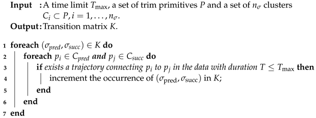
3.4. Identification of Transition Matrix Based on Densities

Let ${\sigma }_1,\dots ,{\sigma }_{n_{\sigma }}$ denote the centers of the trim clusters obtained in the previous step. Now, we draw attention to the computation of maneuvers. As introduced in Definition 4, maneuvers link trims to allow for smooth concatenations of primitives. However, a complete graph would lead to highly inefficient planning. Thus, we define the selection of transitions in the automaton based on their occurrence in the data, i.e., trim cluster ${\sigma }_{\mathrm{pred}}$ is linked to trim cluster ${\sigma }_{\mathrm{succ}}$, if the trims belonging to ${\sigma }_{\mathrm{succ}}$ have been used after (i.e., via connecting maneuvers) the trim members of ${\sigma }_{\mathrm{pred}}$ with high probability.

The probabilities are organized in a transition matrix $K\in {\mathbb{N}}^{n_{\sigma }\times n_{\sigma }}$: for each trim cluster, the transitions from all trim members of this cluster to other clusters are analyzed and summed up and, equivalently, for the transitions to all trim members. Algorithm 1 briefs the occurrences counter for each entry of K.

Algorithm 1: Pseudo-code of the transition matrix occurrences counter.

3.5. Automaton Augmentation by Optimized Maneuvers

Based on the thresholded transition matrix and the trim clusters, the selected maneuvers can be computed optimally with respect to a cost functional. Then, each maneuver with duration T going from a predecessor trim cluster representative ${\sigma }_{\mathrm{pred}}$ to a successor ${\sigma }_{\mathrm{succ}}$ is obtained by solving the following optimal control problem (OCP):

$$\underset{T,x,u}{\mathrm{minimize}}\hspace{1em}J(T,x,u)$$

(7a)

$$\mathrm{subject} \mathrm{to}\hspace{1em}\dot{x}\left(t\right)=f\left(x\right(t),u(t\left)\right), 0<t\le T,$$

(7b)

$$x\left(0\right)=x_0{|}_{{{\sigma }_{\mathrm{pred}}}^{\prime }}$$

(7c)

$$x\left(T\right)=x_T{|}_{{{\sigma }_{\mathrm{succ}}}^{\prime }}$$

(7d)

$$T>0,$$

(7e)

$$0\ge g\left(x\right(t),u(t\left)\right), 0<t\le T,$$

(7f)

with $s_0$ and $s_T$ as fixed states evaluated at the relative equilibria characterized by ${\sigma }_{\mathrm{pred}}$ and ${\sigma }_{\mathrm{succ}}$, respectively, and $g\left(·\right)$ as the constraints for the states and inputs.

4. Autonomous Driving

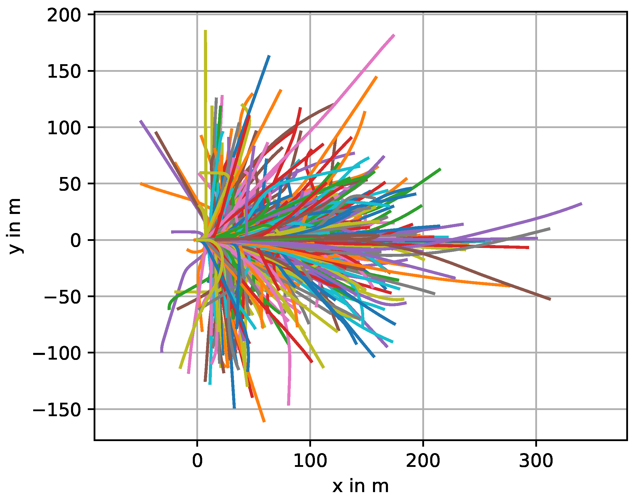
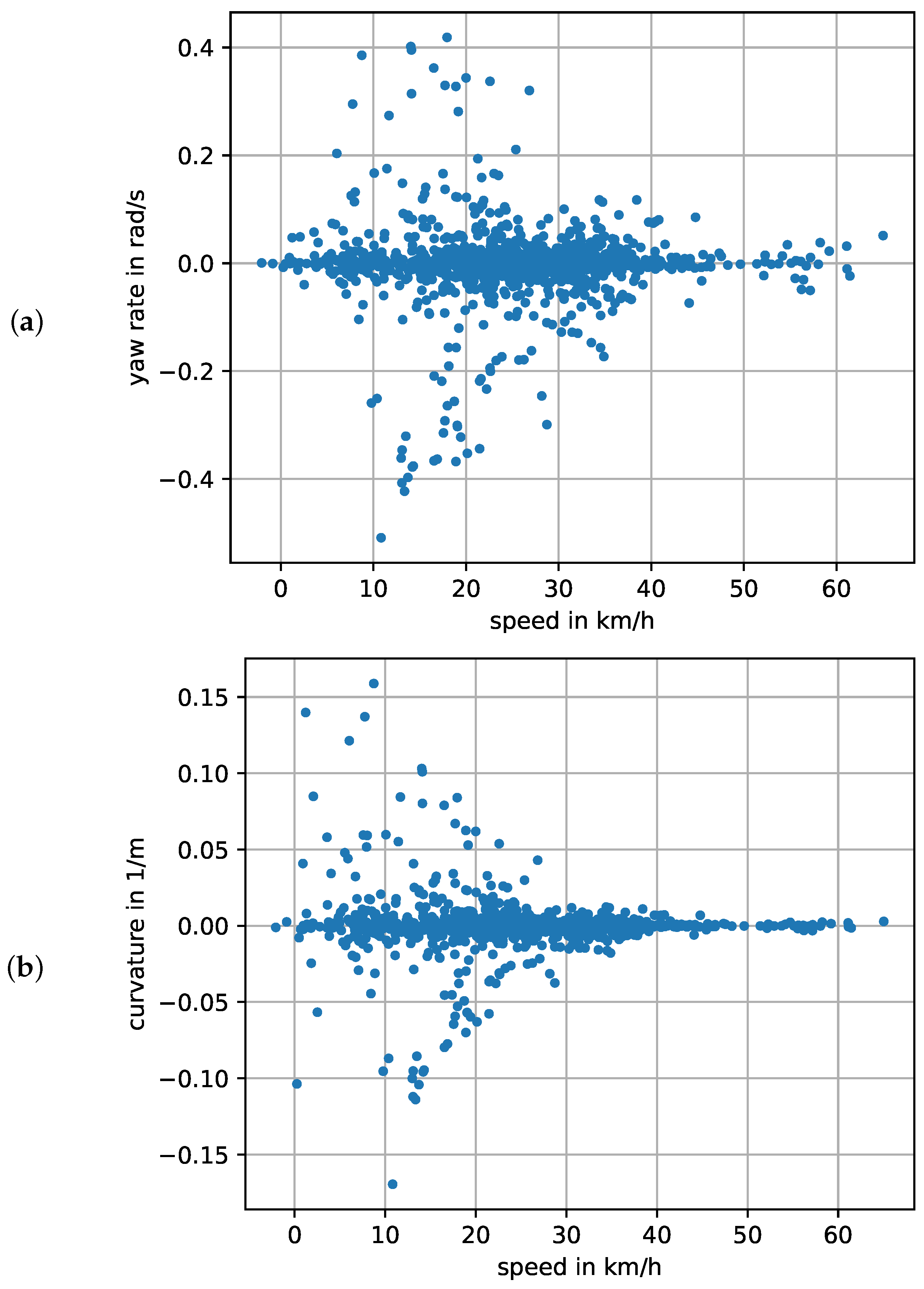
We evaluate the proposed method for trajectory planning in autonomous driving applications showing that it leads to beneficial automata of MP.

4.1. Data

The data used for the numerical examples are taken from the nuScenes data set [47], more specifically from the nuScenes CAN bus expansion. Among other values, it contains information on the pose together with velocity, acceleration, and rotation rate recorded using an inertial measurement unit during urban driving in Singapore and Boston. This data is available for 979 trajectories with a length of 20 $\mathrm{s}$ each, which are depicted in Figure 2. Alternatively, there exists the well known NGSIM data set [48] as well as Ko-PER [49], but both only provide pose data with a relatively low sampling rate from camera and laser scanner data, which are not suitable for the computation of velocities and accelerations. In contrast, nuScenes contains high quality data from an IMU sampled at 50 $\mathrm{Hz}$. It is also free to use for academic purposes.

4.2. Models

Let $p=\left[\begin{array}{ccc}{s}_x& s_y& \psi \end{array}\right]\in {\mathbb{R}}^3$ be the pose, where $s_x$ and $s_y$ are the positions of the center of gravity, and $\psi$ is the vehicle orientation. We consider the state vector given by

$$x=\left[\begin{array}{cc}p& r\end{array}\right]\in {\mathbb{R}}^n,$$

(8)

where r is a vector of $n-3$ states. In addition, let u be the input vector and $f_1(r,u),f_2(r,u),$$f_{\psi }(r,u)$, and $f_r(r,u)$ be arbitrary nonlinear functions. We make the assumption that the model $\dot{x}=f(x,u)$ which corresponds to the data is of the following form:

$$\dot{x}=\left[\begin{array}{c}{\dot{s}}_x\\ {\dot{s}}_y\\ \dot{\psi }\\ \dot{r}\end{array}\right]=\left[\begin{array}{c}{f}_1(r,u)cos(f_2(r,u)+\psi )\\ f_1(r,u)sin(f_2(r,u)+\psi )\\ f_{\psi }(r,u)\\ f_r(r,u)\end{array}\right].$$

(9)

Proposition 2.

The symmetry group for (9) is given by combined rotations and translations on the pose, i.e.,

$$\mathcal{G}:=\left\{g\in \mathsf{SE}\left(n\right):g:=g(\Delta x)=\left[\begin{array}{cc}R& \Delta x\\ 0& 1\end{array}\right]\right\},$$

(10)

where

$$\begin{array}{cc}\hfill & \begin{array}{c}\hfill R=\left[\begin{array}{cc}{R}_{\mathsf{SO}\left(3\right)}& 0\\ 0& I\end{array}\right]\in \mathsf{SO}\left(n\right),\end{array}\hfill \end{array}$$

(11)

$$\begin{array}{cc}\hfill & \begin{array}{c}\hfill \Delta x=\left[\begin{array}{c}\Delta s_x\\ \Delta s_y\\ \Delta \psi \\ 0\end{array}\right]\in {\mathbb{R}}^2\times S^1\times {\left\{0\right\}}^{n-3},\end{array}\hfill \end{array}$$

(12)

$$\begin{array}{cc}\hfill & \begin{array}{c}\hfill R_{\mathsf{SO}\left(3\right)}=\left[\begin{array}{ccc}cos(\Delta \psi )& -sin(\Delta \psi )& 0\\ sin(\Delta \psi )& cos(\Delta \psi )& 0\\ 0& 0& 1\end{array}\right]\in \mathsf{SO}\left(3\right),\end{array}\hfill \end{array}$$

(13)

for I being the identity matrix with appropriate dimension, a vector $\Delta x$, and g given in homogeneous coordinates, such that the the affine-linear group action can be represented by:

$${\Psi }_g\left(x\right)=Rx+\Delta x.$$

(14)

Proof. 

The proof is given in Appendix A. □

Many vehicle models assume the generic configuration represented by (9), e.g., the kinematic single-track, single-track, single-track drift, and multi-body models presented in [50]. We chose to use the kinematic bicycle model from [50], characterized by the state vector:

$$x={\left[\begin{array}{ccccc}{s}_x& s_y& \psi & v& \delta \end{array}\right]}^{\mathrm{T}}\in {\mathbb{R}}^5,$$

(15)

and the input vector:

$$u={[u_v\hspace{1em}{u}_{\delta }]}^{\mathrm{T}}\in {\mathbb{R}}^2,$$

(16)

where $s_x$ and $s_y$ are the positions of the rear axis, $\psi$ is the vehicle orientation, v is the velocity vector, $\delta$ is the steering angle, $u_v$ is the longitudinal acceleration, and $u_{\delta }$ is the velocity of the steering angle. The state space equations are given by:

$$\left\{\begin{array}{cc}\hfill {\dot{s}}_x\left(t\right)& =v\left(t\right)·cos\left(\psi \right(t\left)\right),\hfill \\ \hfill {\dot{s}}_y\left(t\right)& =v\left(t\right)·sin\left(\psi \right(t\left)\right),\hfill \\ \hfill \dot{\psi }\left(t\right)& =\frac{v\left(t\right)}{L}·tan\left(\delta \left(t\right)\right),\hfill \\ \hfill \dot{v}\left(t\right)& =\left(t\right),\hfill \\ \hfill \dot{\delta }\left(t\right)& =\left(t\right),\hfill \end{array}\right.$$

(17)

for L being the wheelbase with value $2.588$ $\mathrm{m}$, reference for the Renault Zoe used in obtaining the nuScenes data [51]. For this model, the parameters that characterize a trim primitive are the velocity and the yaw rate when “trimmed”.

4.3. Numerical Examples

The trajectory data needed to extract trim primitives can be obtained from the nuScenes data set. Acceleration data is available from the inertial measurement data, but the values are sometimes non-zero although the car is standing still. This could be caused by the effect of gravity on the sensor on tilted terrain. Thus, we obtain the acceleration data, as well as the derivative of the yaw rate, using finite differences. Both the velocity and the rotation rate data have to be smoothed before the derivatives could be calculated to get rid of noise. This smoothing was accomplished by a convolution with a box function, which was 134 time points wide for the yaw rate and 17 time points for the velocity. Convolution with a box function results in a running average.

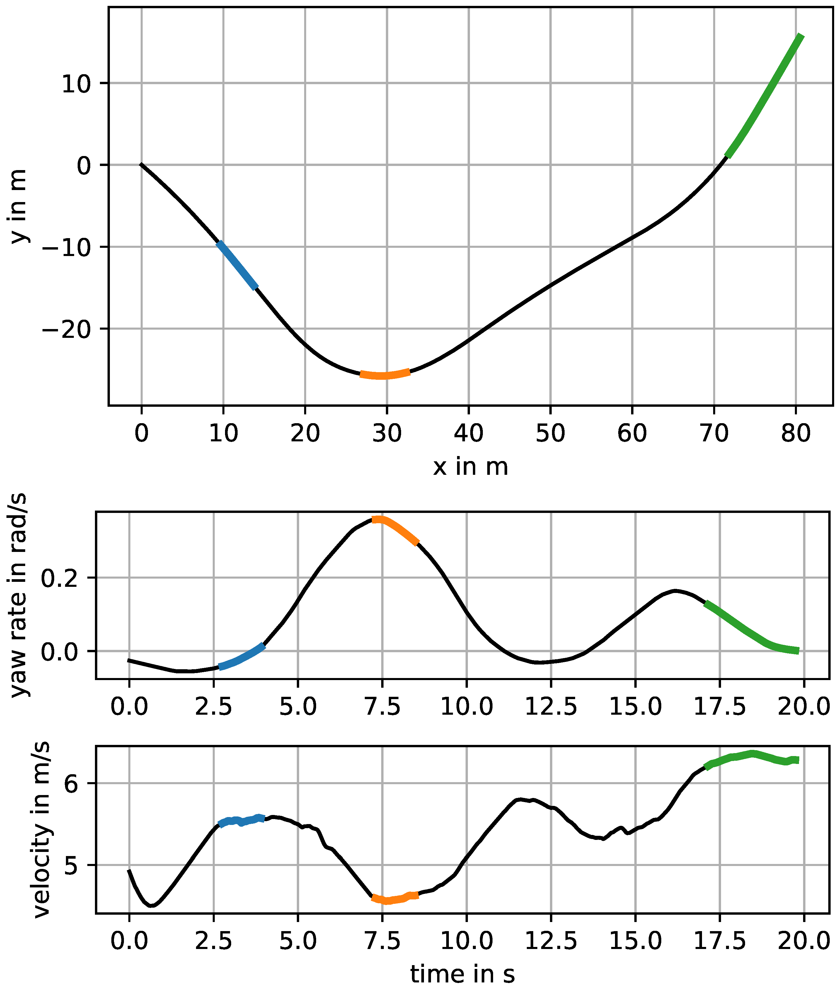
4.3.1. Trim Detection

Instead of directly applying Corollary 2, we further exploit the structure of the trims obtained from the used model. Due to the second-order equations, trims necessarily have to be uncontrolled, i.e., $u_i^k=0$. Moreover, along a trim, both the acceleration and the yaw rate have to vanish. Thus, we scan individual data sets for

$$\left|\frac{v_{i+1}^k-v_i^k}{t_{i+1}^k-t_i^k}\right|<{ϵ}_v\mathrm{and}\left|\frac{{\dot{\psi }}_{i+1}^k-{\dot{\psi }}_i^k}{t_{i+1}^k-t_i^k}\right|<{ϵ}_{\dot{\psi }}.$$

The considered tolerance for absolute acceleration is ${ϵ}_v=$ $0.2 \mathrm{m}/{\mathrm{s}}^2$ and for the derivative of the yaw rate, ${ϵ}_{\psi }=$ $0.08 \mathrm{rad}/{\mathrm{s}}^2$. Parts of the trajectory which satisfy these conditions for a minimal duration of 1 $\mathrm{s}$ are considered to be trim trajectories. The mean velocity and mean yaw rate are then stored for the next step of the process. A trajectory with the trim parts marked can be seen in Figure 3.

The trim detection finds 1460 trim trajectories, which means that each trajectory contains 1.49 trims on average. The average duration is $2.17$ $\mathrm{s}$. The distribution of the parameters of the detected trims, velocity, and yaw rate is depicted in Figure 4a.

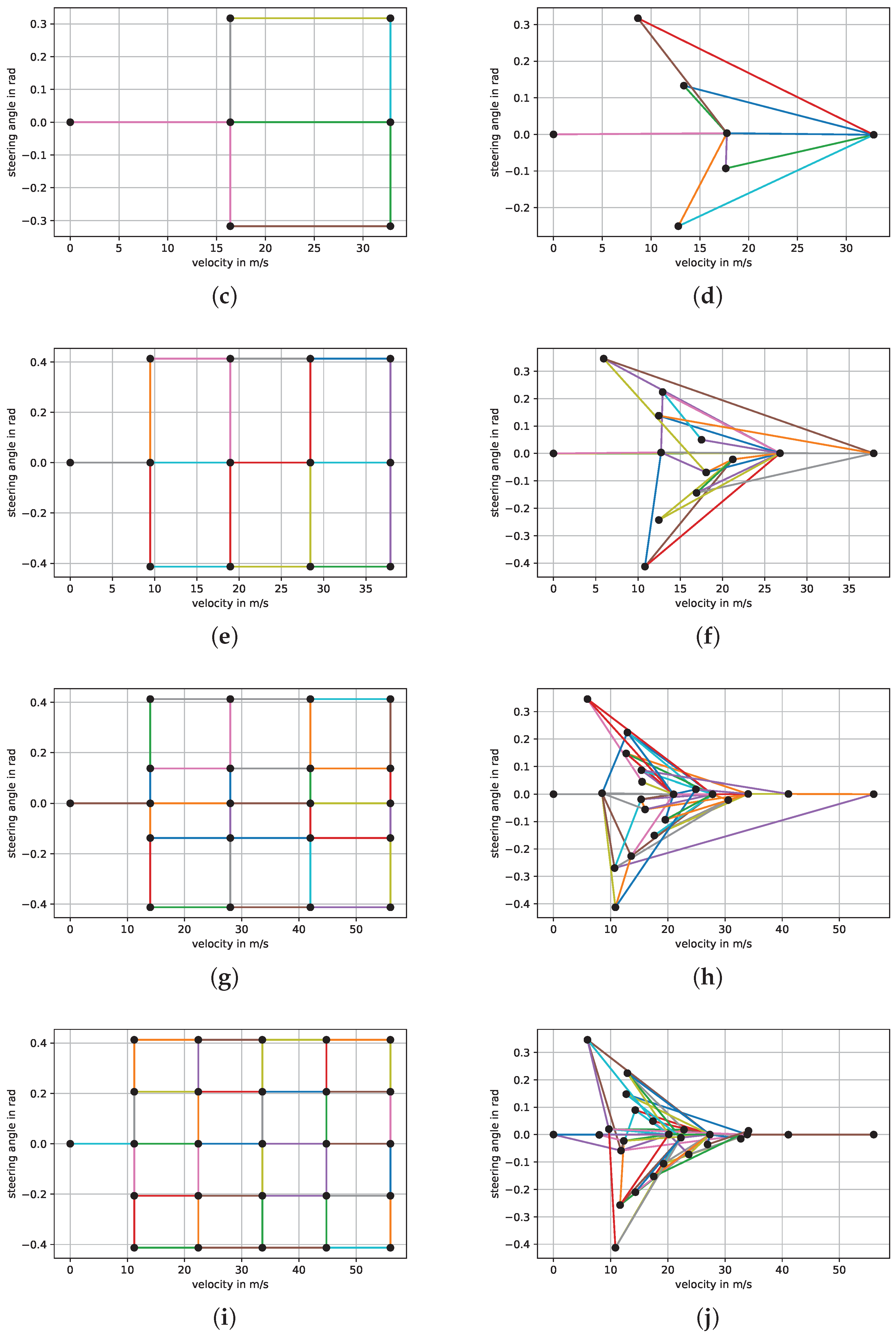
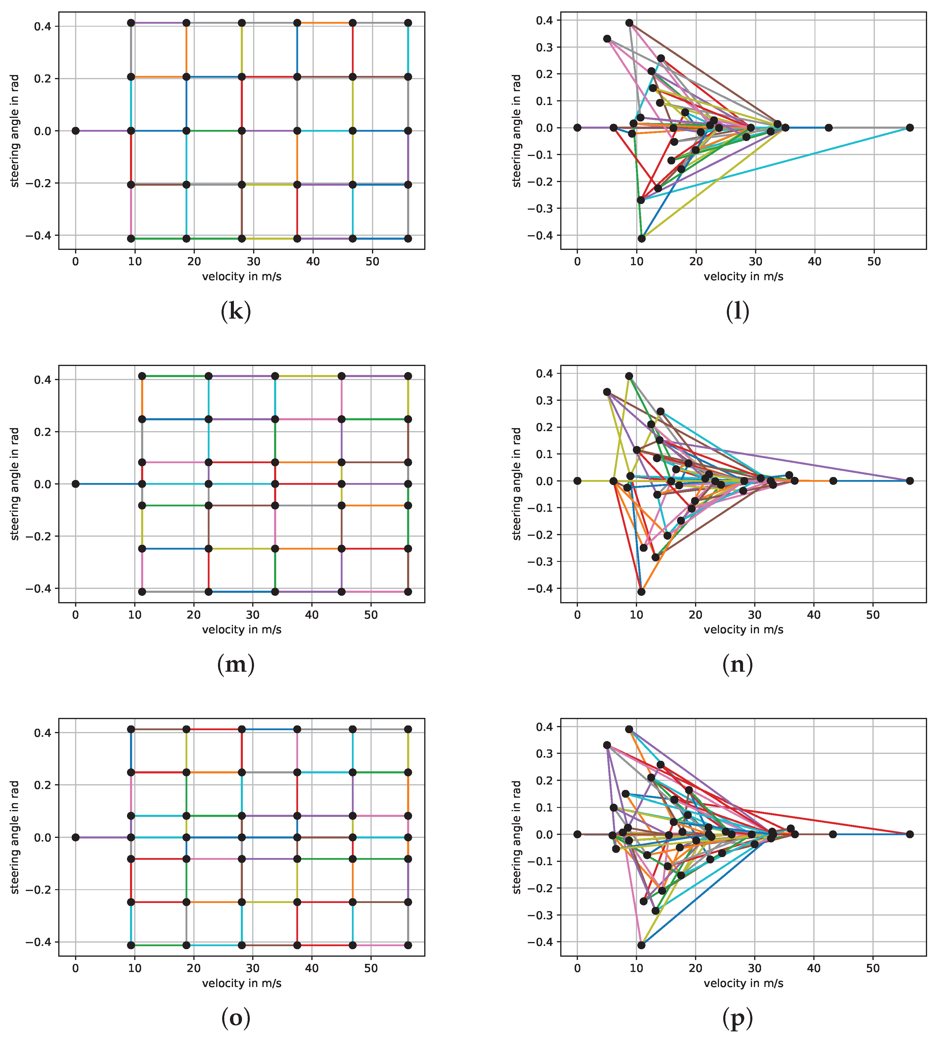
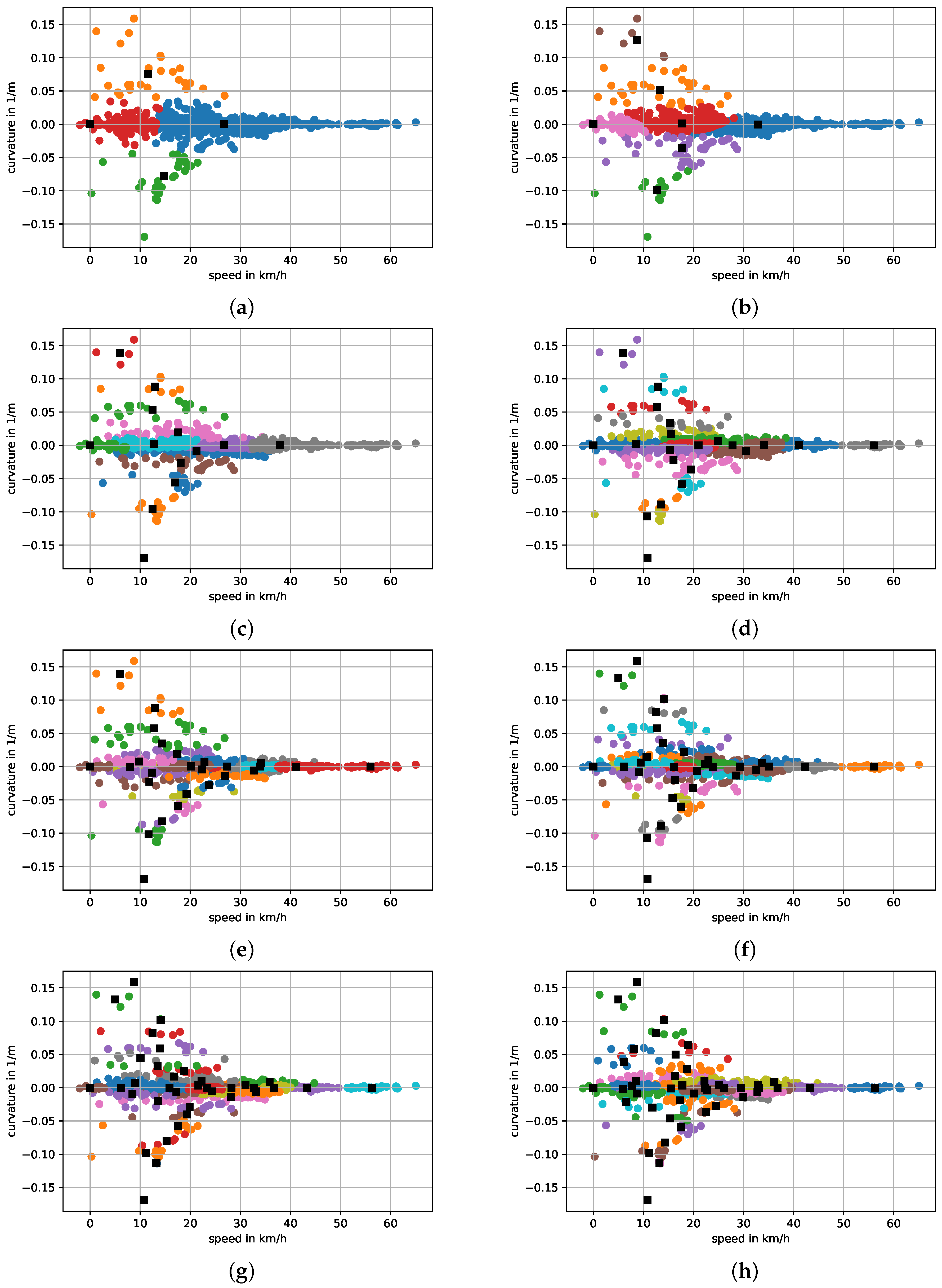
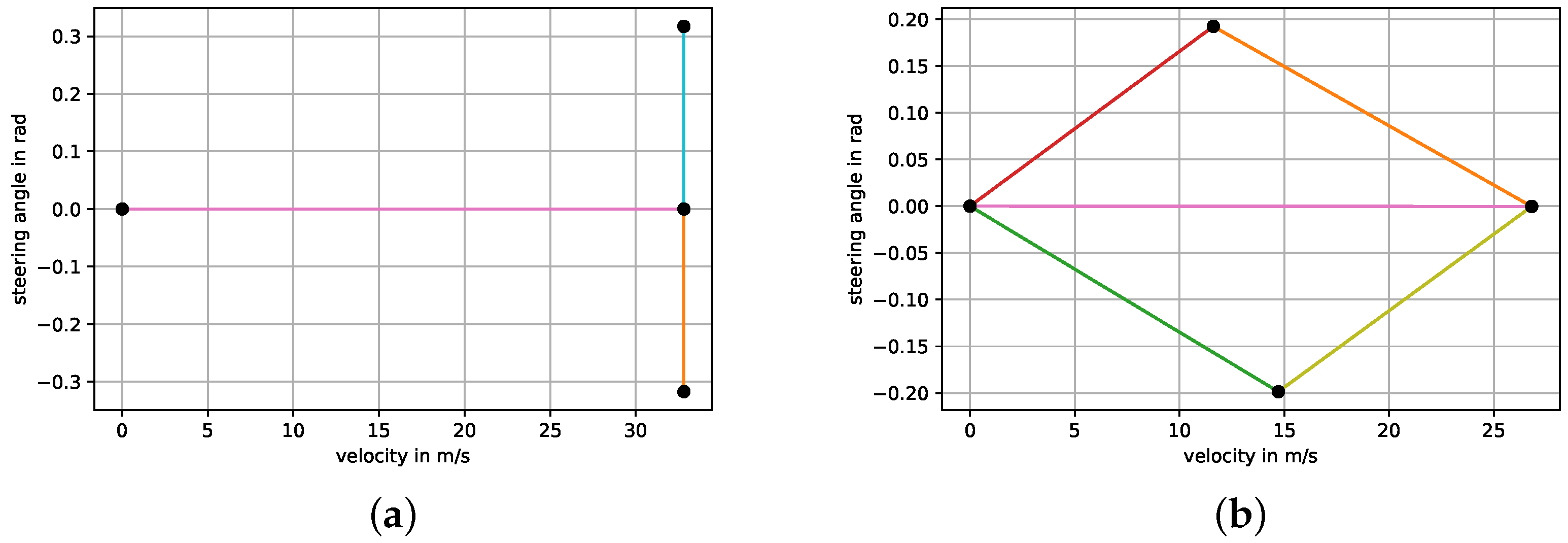
4.3.2. Trim Clustering

As the clustering is accomplished using the k-means algorithm, the number of clusters is a hyperparameter that must be chosen. To compute k-means, we used the scikit-learn package [52]. The initial clusters’ centers were selected for a faster convergence through the k-means++ technique [53].

While searching for parts of a trajectory with numerically constant velocity and yaw rate is suitable for detecting trims in data, other pairs of constant parameters characterizing a trim exist. For example, velocity and curvature of the curve travelled by the point $(s_x,s_y)$ uniquely define a trim up to the coasting time. The distribution of those features is shown in Figure 4b. This signed curvature is also given by $\kappa =\dot{\psi }/v$, with v being the velocity of $(s_x,s_y)$. It is independent of the speed at which the car travels, and in purely kinematic car models, it is directly related to the steering angle.

The features used for clustering are the velocity and the curvature. As the k-means algorithm uses Euclidean distance as a closeness metric, the features are normalized by dividing the values by their standard deviation. They are then multiplied by importance factors, which are one for the velocity and three for the curvature. Choosing a higher importance factor for the curvature results in more cluster centers at higher curvatures can improve automaton quality, counteracting the phenomenon that there are relatively few detected trims with a high steering curvature. The standstill trim, i.e. with $v=0$ and $\kappa =0$, was added artificially after the clustering process, followed by relabeling each point, since it enables braking and stopping in the motion planning.

We choose eight different configurations for the automata: with 4, 7, 13, 21, 26, 31, 36 and 43 trim primitives. The choice of these quantities was made to match the number of trims of handcrafted automata, as it will be shown in Section 4.4. The results can be seen in Figure 5.

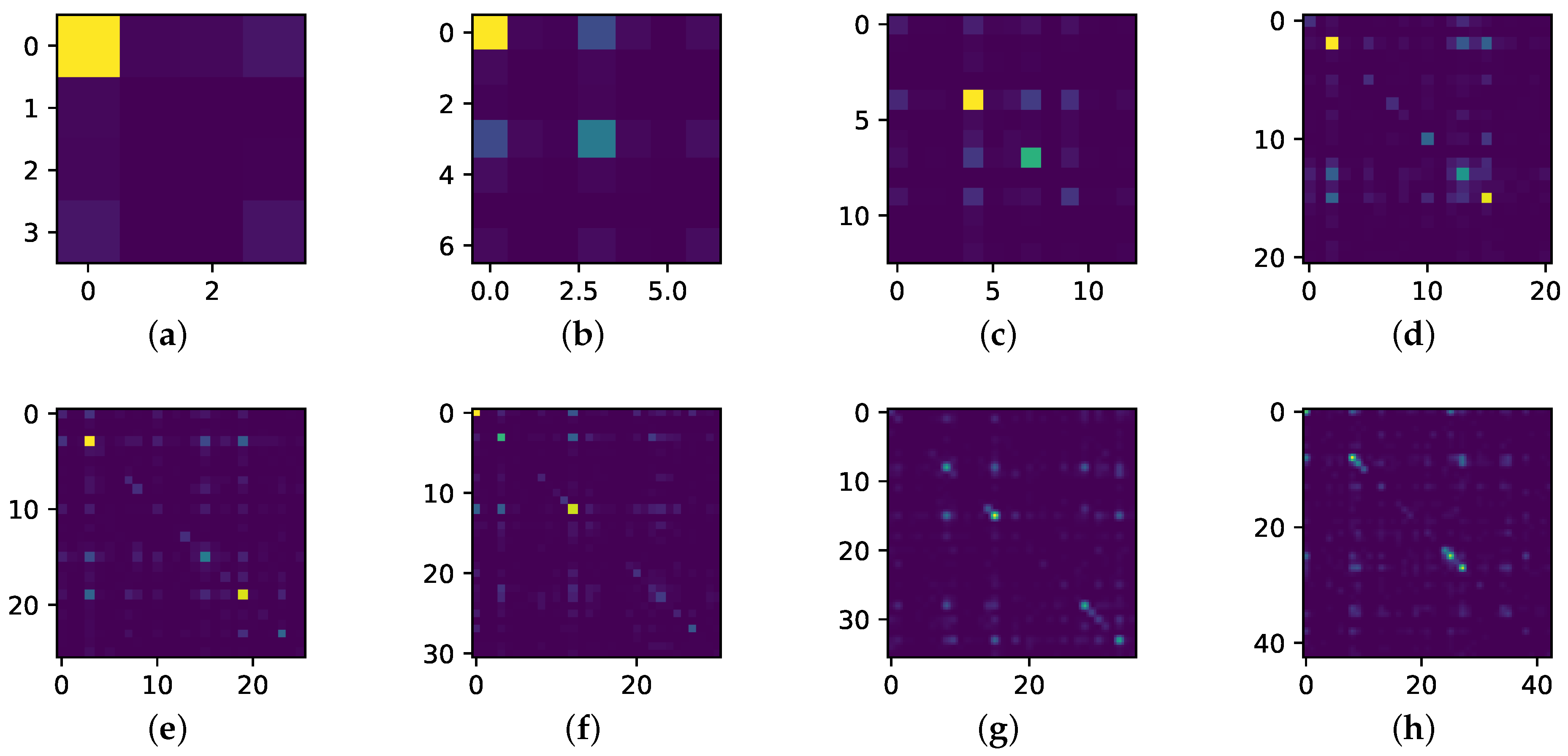
4.3.3. Transition Matrix

In Section 3.4, the transition matrix was introduced to analyze the statistics of two trims being used subsequently within trajectory data. In Figure 6, the resulting matrices are given for the selected automata. For each cluster, at least the two outgoing and the two incoming edges of highest probability are added to the automaton graph as maneuvers. Each maneuver’s state and control trajectory was then determined by solving an optimal control problem, minimizing the time.

4.3.4. Computation of Maneuvers

We obtained the maneuvers solving the OCP (7) as:

$$\mathrm{minimize}\hspace{1em}T$$

(18a)

$$\mathrm{subject}\hspace{1em}\mathrm{to}\hspace{1em}\dot{x}\left(t\right)=f\left(x\right(t),u(t\left)\right),$$

(18b)

$$x(0)={\left[\begin{array}{ccccc}0& 0& 0& v_{\mathrm{pred}}& {\delta }_{\mathrm{pred}}\end{array}\right]}^{\mathrm{T}},$$

(18c)

$$v(T)=v_{\mathrm{succ}},$$

(18d)

$$\delta (T)={\delta }_{\mathrm{succ}},$$

(18e)

$$T\ge 0.1,$$

(18f)

$$\underline{u_{\dot{v}}}\le u_{\dot{v}}(t)\le \stackrel{̲}{u_{\dot{v}}},$$

(18g)

$$\underline{u_{\dot{\delta }}}\le u_{\dot{\delta }}(t)\le \stackrel{̲}{u_{\dot{\delta }}},$$

(18h)

$$\underline{v}\le v(t)\le \stackrel{̲}{v},$$

(18i)

$$\underline{\delta }\le \delta (t)\le \stackrel{̲}{\delta },$$

(18j)

$$u_{\dot{v}}(t)·v(t)\le \stackrel{̲}{u_{\dot{v}}}·\tilde{v}$$

(18k)

The minimum duration in (18f) was set to $0.1$ $\mathrm{s}$ for not slowing down the graph search, specifically the chosen ∏* search. Computation (18k) models the engine power’s limit of a vehicle, where $\tilde{v}$ is a switching velocity. Lower and upper bars represent, respectively, minimum values and maximum values for the variables given in

Table 1. Parameters of the optimization problem (18).

Param.	Value	Param.	Value	Param.	Value
$\underline{u_{\dot{v}}}$	−11.5 m ${\mathrm{s}}^{-2}$	$\underline{u_{\dot{\delta }}}$	−0.4 ${\mathrm{s}}^{-1}$	$\underline{\delta }$	−0.91
$\stackrel{̲}{u_{\dot{v}}}$	11.5 m ${\mathrm{s}}^{-2}$	$\stackrel{̲}{u_{\dot{\delta }}}$	0.4 ${\mathrm{s}}^{-1}$	$\overline{\delta }$	0.91
$\underline{v}$	−13.9 m ${\mathrm{s}}^{-1}$	$\overline{v}$	45.8 m ${\mathrm{s}}^{-1}$	$\tilde{v}$	4.755 m ${\mathrm{s}}^{-1}$

. These constraints are taken from the model description in [50].

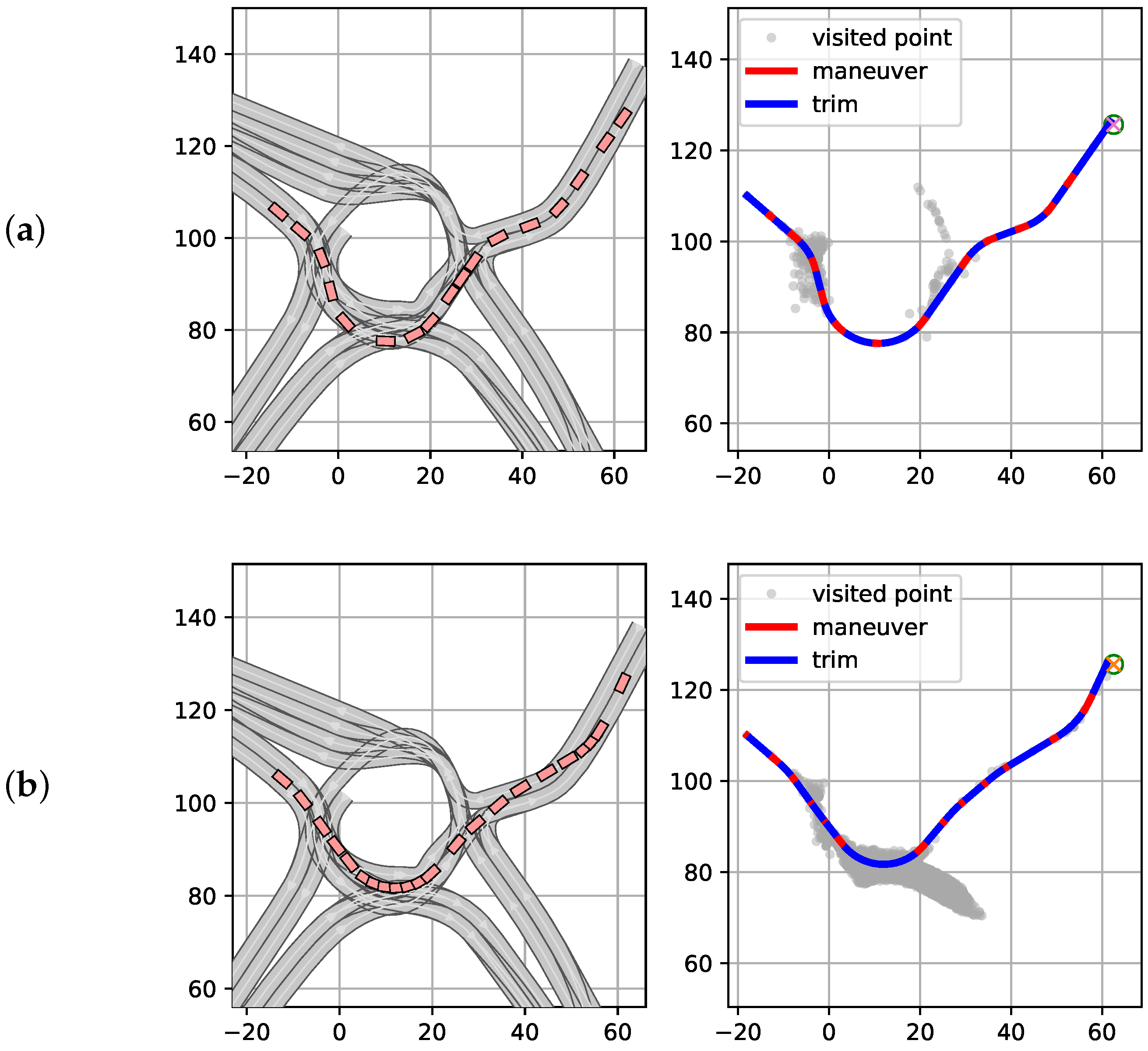
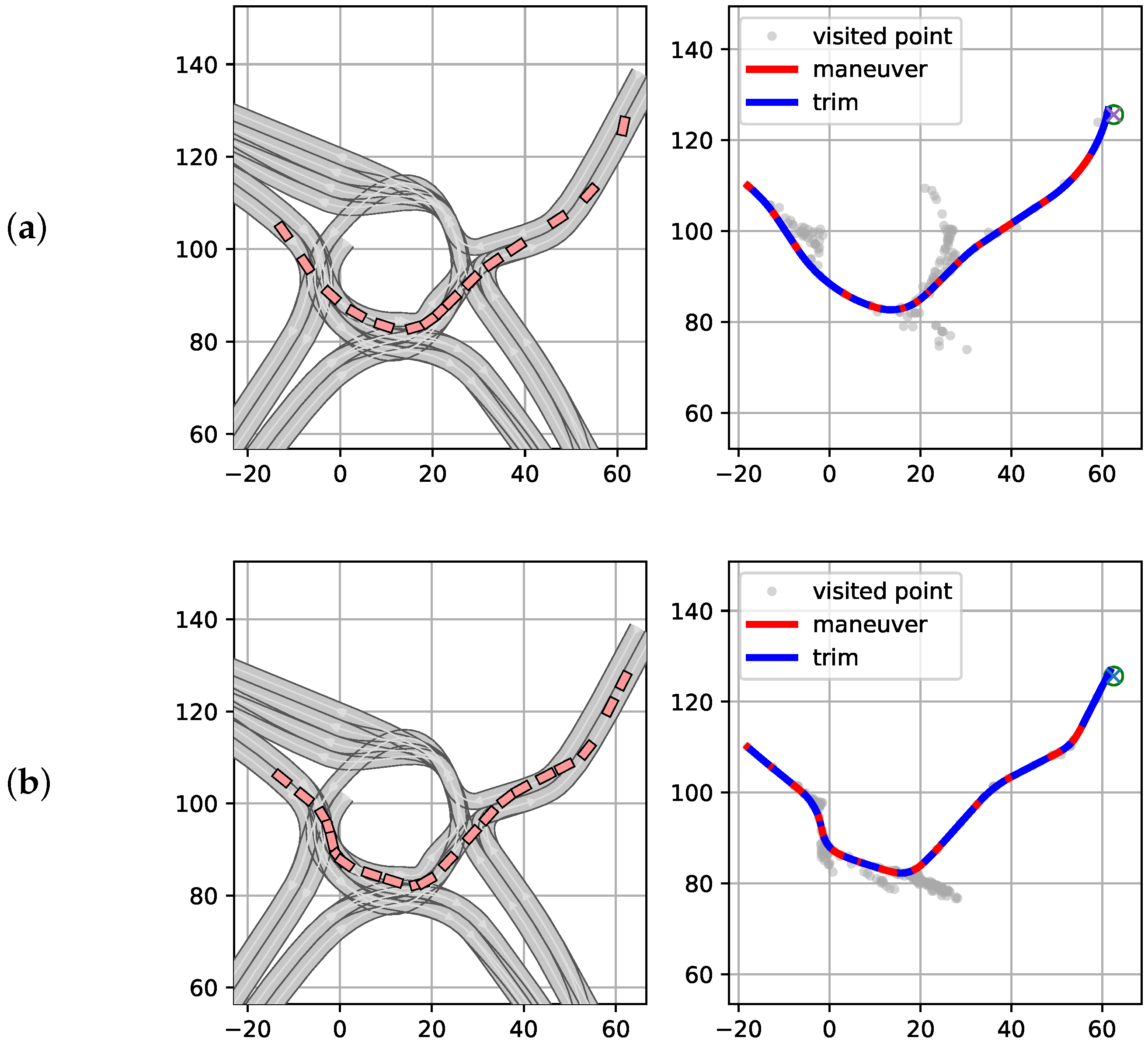
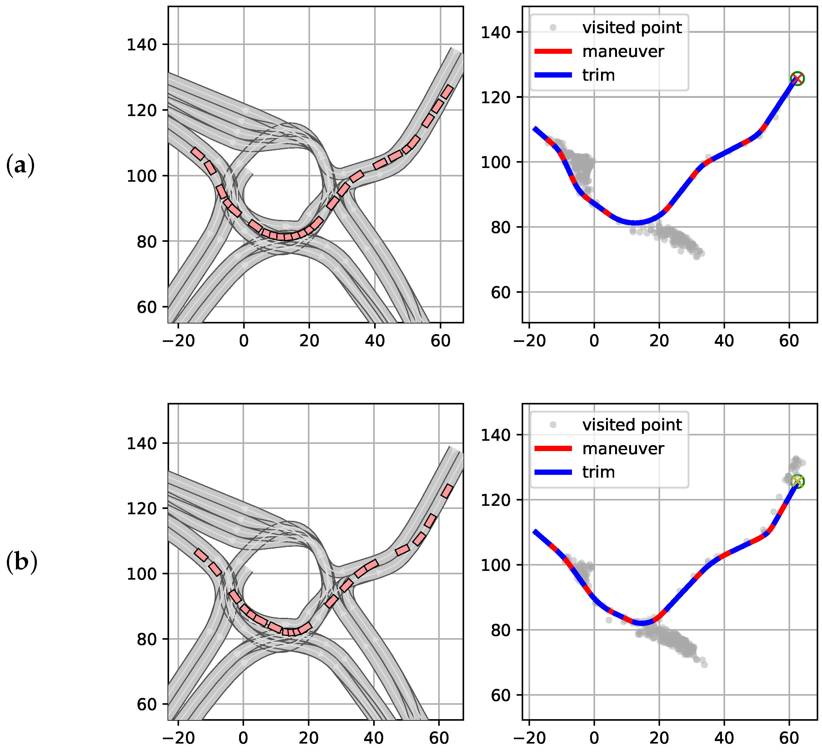
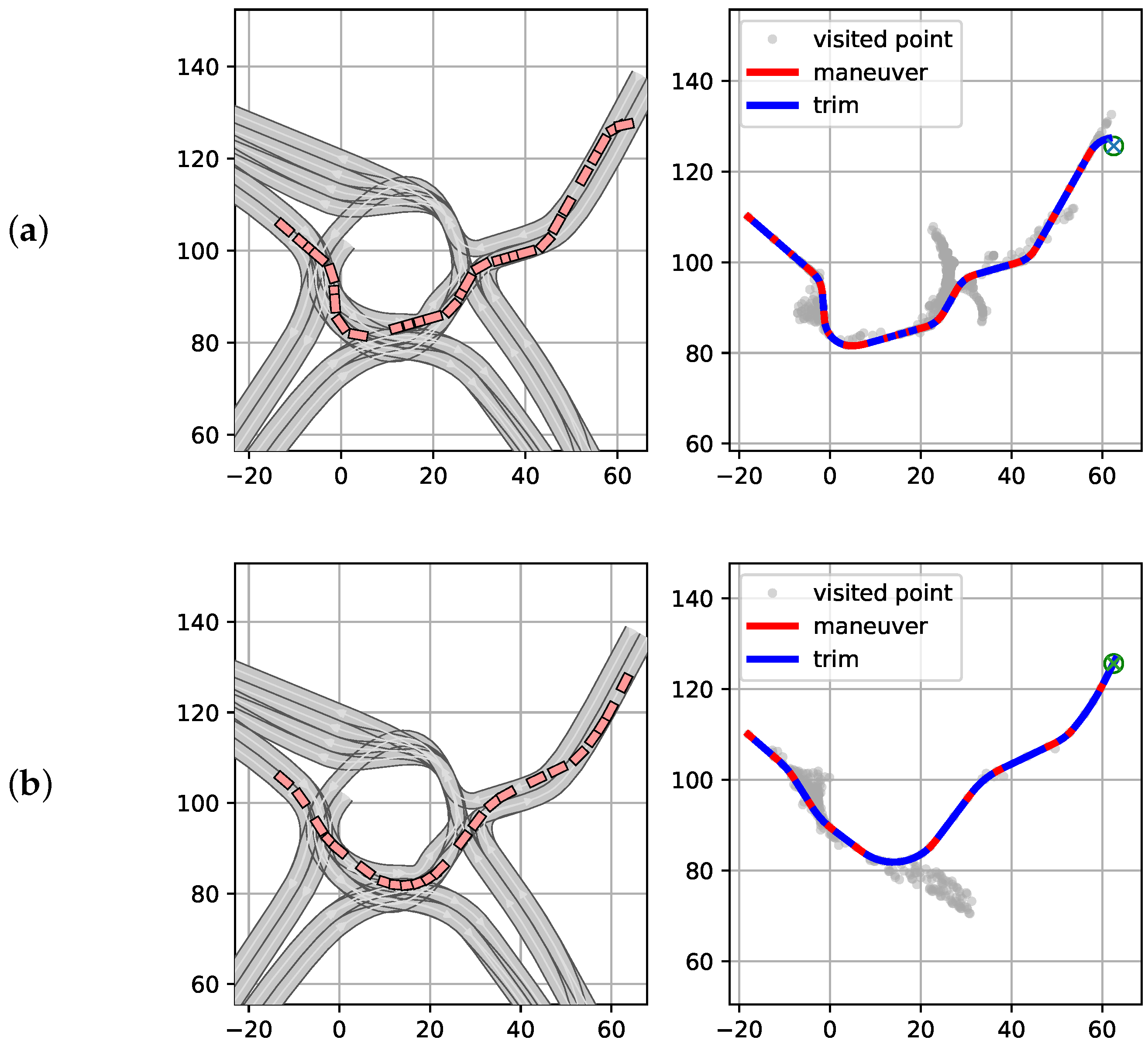
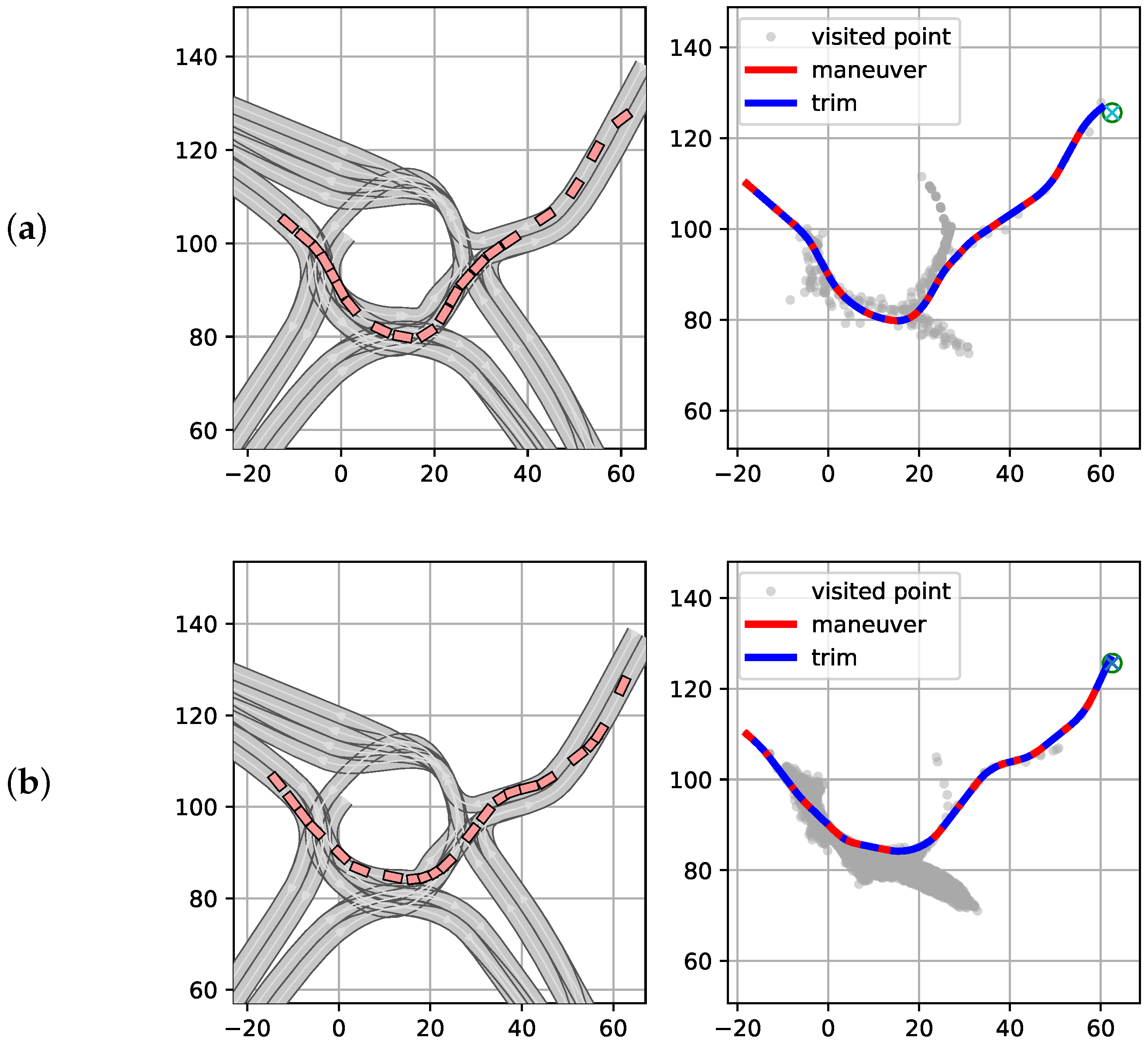
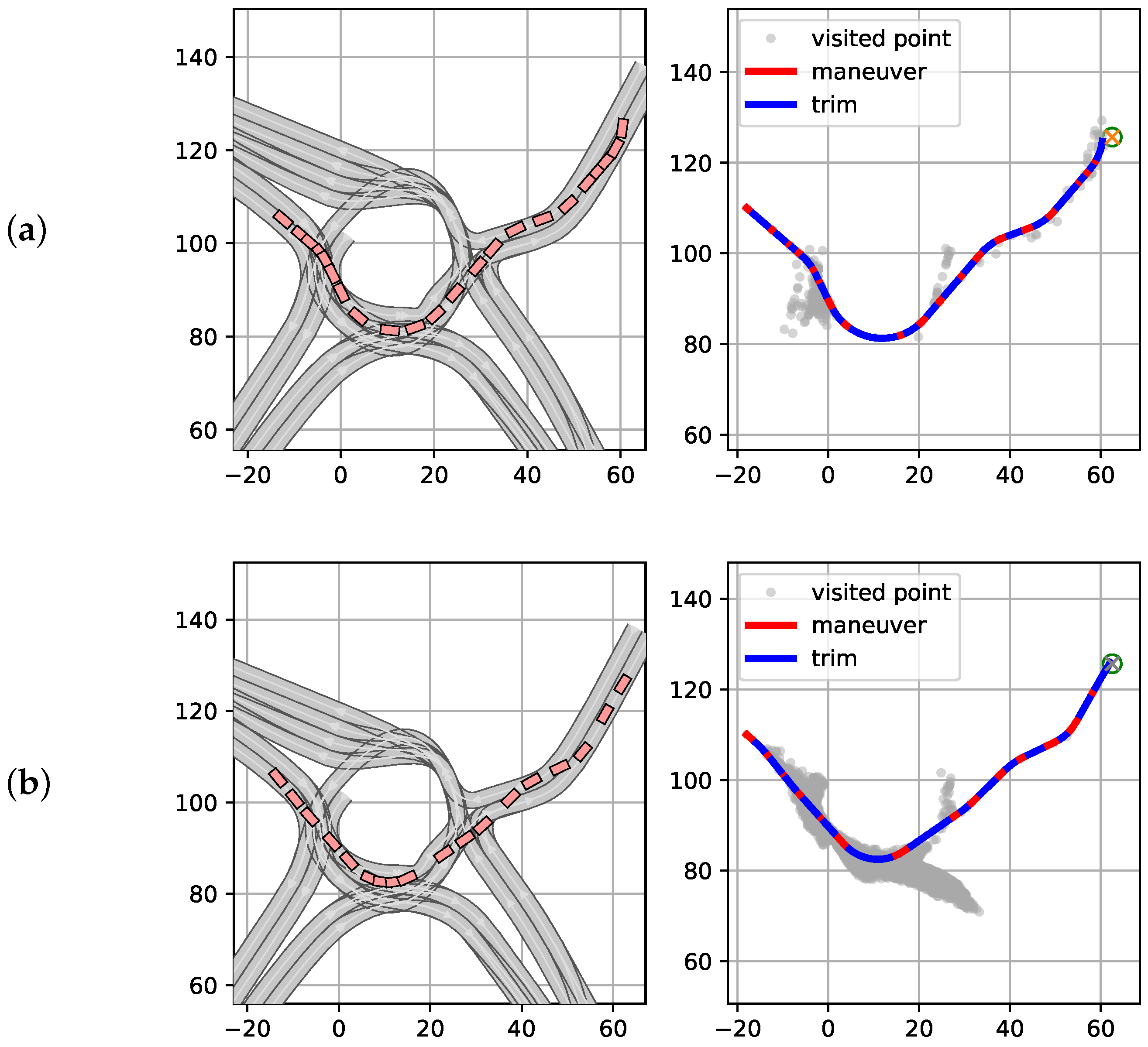
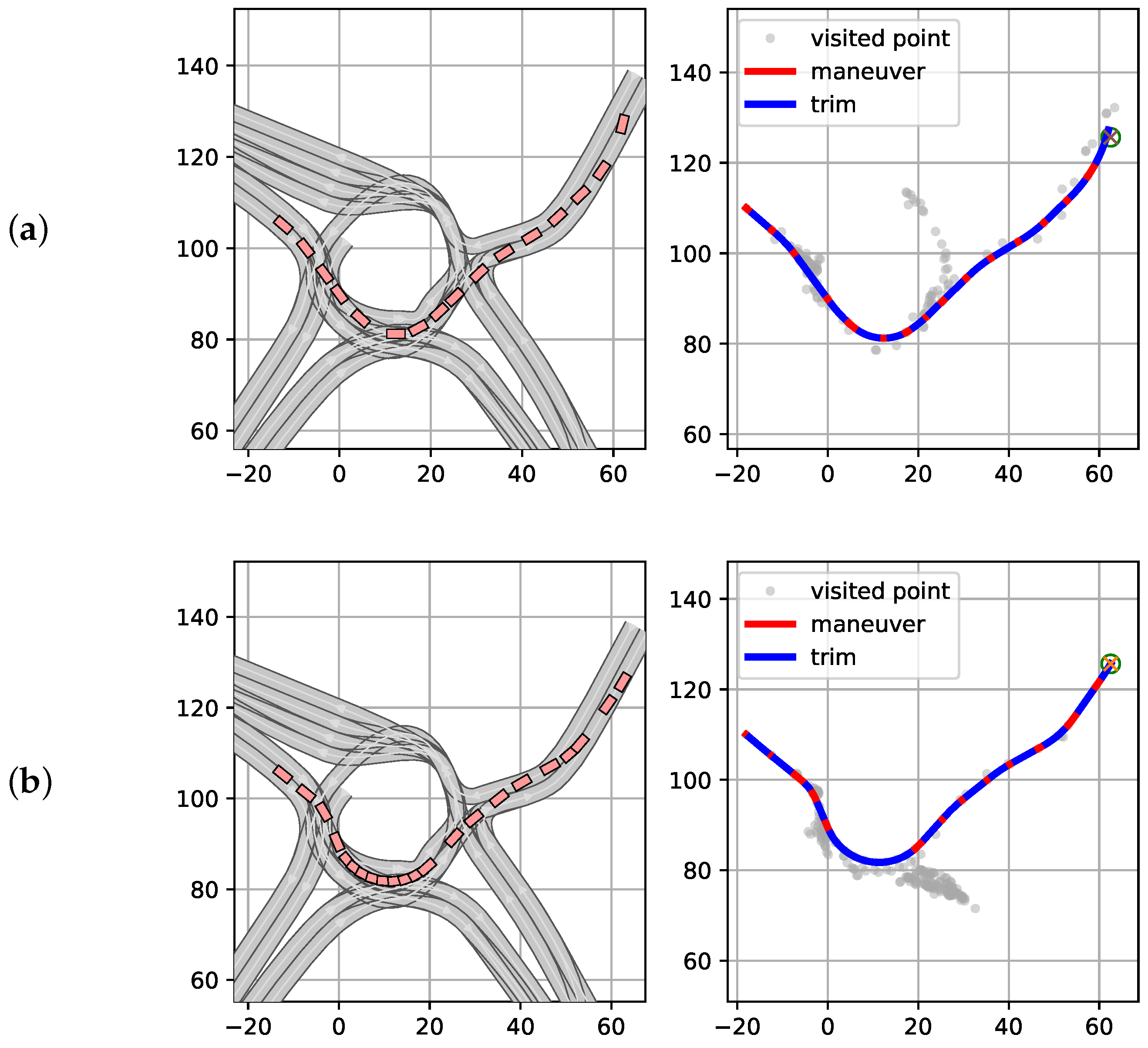
4.4. Validation of the Automata

We choose a region in the Boston seaport, one of the places where nuScenes collected data, to validate our automata. We generated a simulated scenario based on the real map using CommonRoad’s converter and Scenario Designer [54,55]. The initial and final positions for the motion planning problem were extracted from a nuScene’s trajectory on this map, which can be seen in Figure 7.

For verifying the results, we compare the extracted automata with handcrafted ones. When there is not any real-world data available for the construction of automata, one pragmatic, yet efficient way to design the automaton is by an equally spread grid covering the entire space of allowed velocities and steering angles for the model [4]. However, for a fair comparison, we chose a grid of trims covering the same range of steering angles and velocities as the extracted automata. Moreover, the handcrafted and extracted automata have the same quantity of trims, and the numbers of maneuvers match as closely as possible. Figure 8 shows the resulting automata for the handcrafted and the extracted versions, where each coloured line represents at least one existent maneuver relating the trims, denoted by black squares. For the handcrafted ones, the lines are specifically two maneuvers in opposite directions. Different colors were used just to identify distinct relationships between trims.

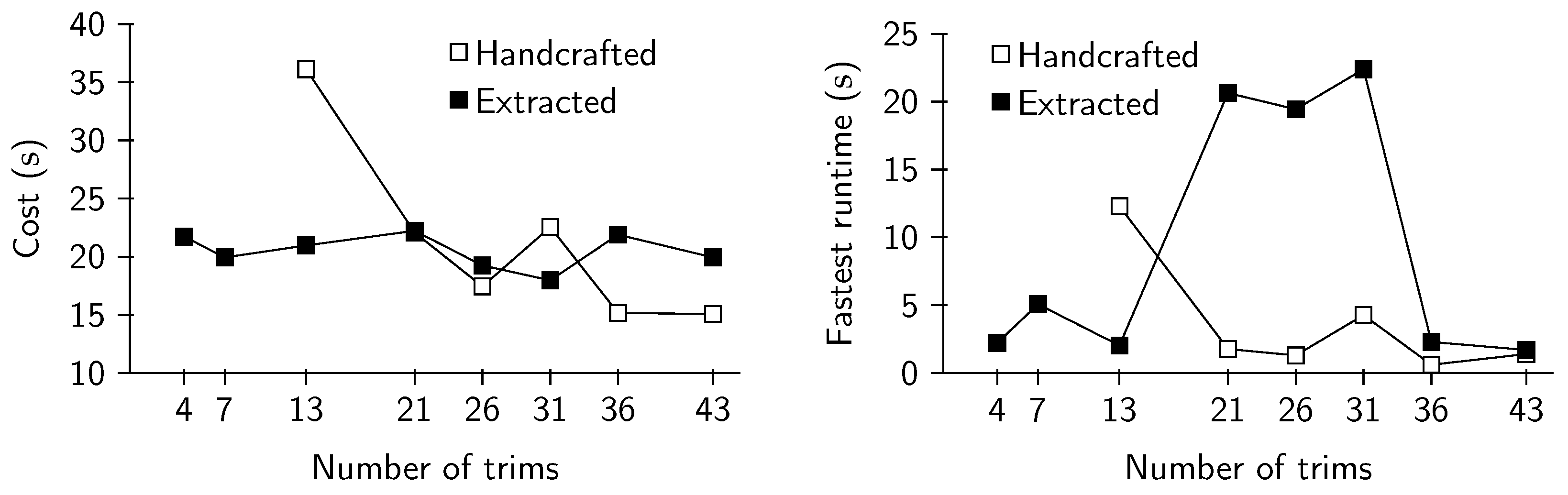
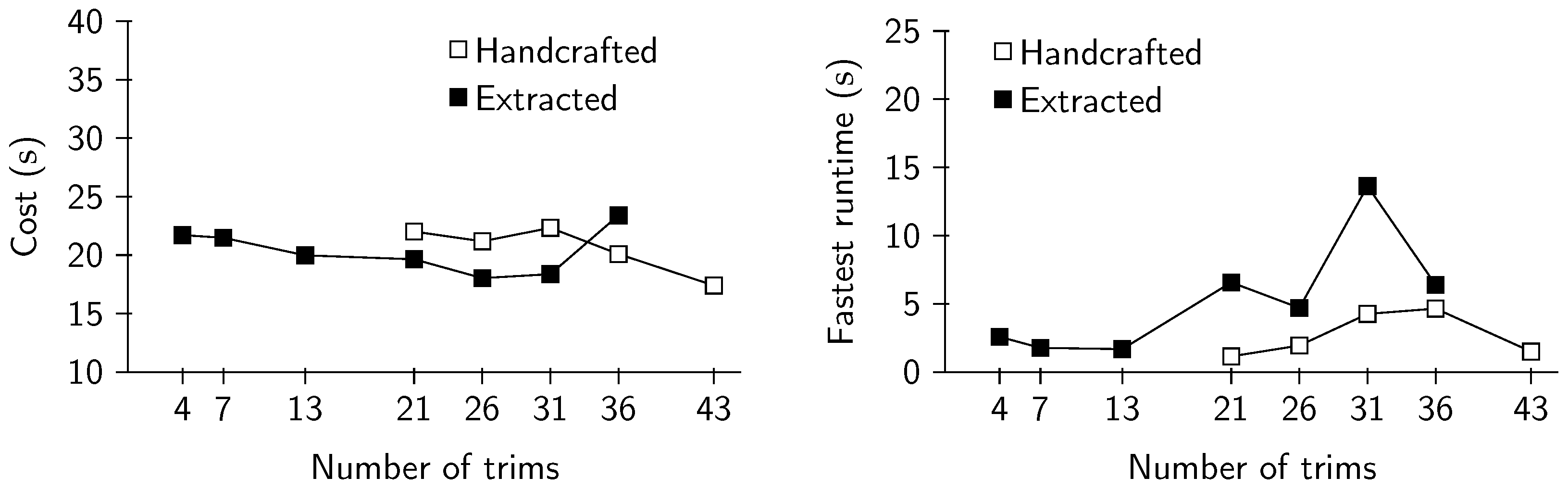
4.5. Evaluation in Simulation and Discussion

We tested the motion planning problem in a Windows 11 workstation with 1.90 GHz Intel^® Core^™ i7 CPU and 16 GB RAM using the CommonRoad benchmark [50]. For the motion planning problem, we used the ∏* algorithm, described in [4], in which the search is performed for trim primitives with fixed duration, and, then, it is possible to optimize their durations to match an exact goal pose if the node is inside an allowed optimization region. The ∏* search presented the following parameters:

• The trajectory’s duration as the cost for the search;
• Fixed trim’s duration of $0.7$ $\mathrm{s}$;
• Timeout of 60 $\mathrm{s}$;
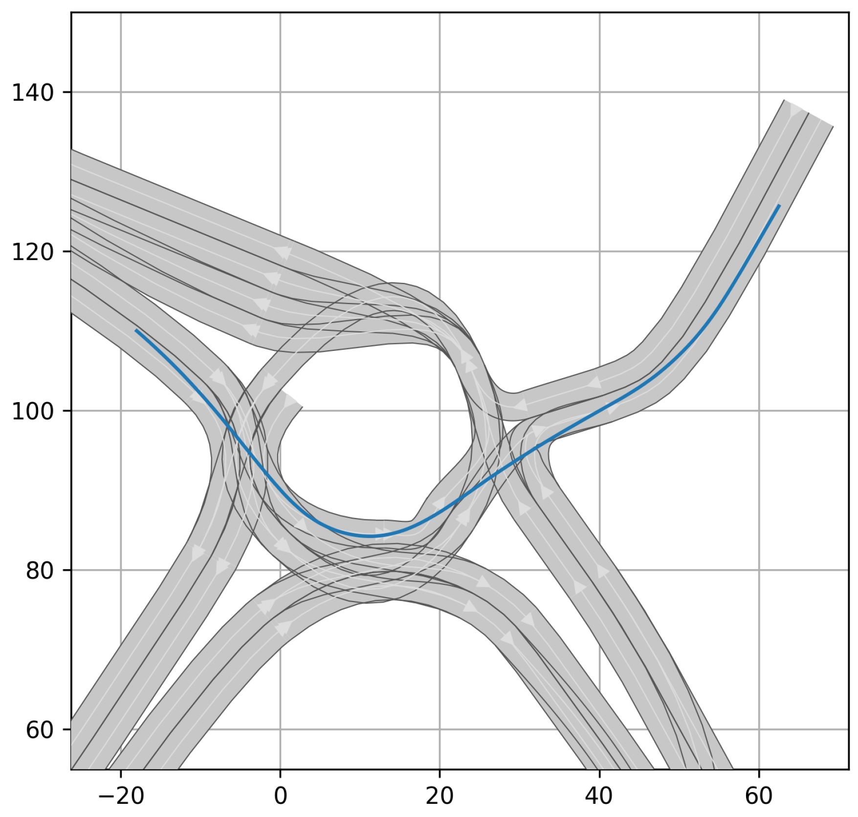
• As mentioned previously in Section 4.4, the initial and goal pose were extracted from the data’s trajectory depicted in Figure 7, and the vehicle is initially stopped;
• Goal region as the circle with radius of 2 $\mathrm{m}$ centered in the goal position;
• Optimization region in a radius of 30 $\mathrm{m}$ from the goal;
• The inflation factor and heuristics were the same as in [4].

The numerical results are given in

Table 2. Results for the handcrafted and extracted automata.

Type	Trims	Maneuvers	Cost (s)	Runtime (s)
Handcrafted	4	10	–	$>60$
Extracted	4	14	$21.73$	$2.23$
Handcrafted	7	23	–	$>60$
Extracted	7	27	$19.94$	$5.07$
Handcrafted	13	49	$36.12$	$12.30$
Extracted	13	53	$20.97$	$2.03$
Handcrafted	21	85	$22.08$	$1.77$
Extracted	21	85	$22.23$	$20.64$
Handcrafted	26	108	$17.45$	$1.30$
Extracted	26	106	$19.25$	$19.44$
Handcrafted	31	131	$22.55$	$4.27$
Extracted	31	129	$17.97$	$22.39$
Handcrafted	36	154	$15.16$	$0.61$
Extracted	36	151	$21.90$	$2.29$
Handcrafted	43	187	$15.08$	$1.40$
Extracted	43	174	$19.94$	$1.70$

and Figure 9, with relative trajectories depicted in Figures 11–17. The algorithm’s times presented on the table reflect the fastest running time found in each case.

No trend in the computation times in Table 2 can be observed. For 21, 26, and 31 trims, the extracted automata explored many nodes on the second exit of the roundabout that resulted in higher runtimes. This peculiarity is also due to the characteristics of the chosen test scenario, the planning algorithm, and its parameters. In fact, it was observed empirically that the results are significantly sensitive to the parameters of the ∏* search. To illustrate it, we solved the same problem just increasing the trim’s duration by $0.05$ $\mathrm{s}$, with the results presented in Figure 10. Thus, the adjustment of these variables should be carefully performed to solve the planning problem. This paper does not intend to perform a full quantitative investigation of the results and sensitivity analysis, which is due more to the motion planning algorithm than to the automata themselves. Instead, we are focused on a qualitative analysis of different automata.

Interestingly, extracted trims caused a relatively constant cost, i.e., the duration of the whole trajectory. In contrast, the cost tends to decrease as the handcrafted automaton’s size increased, which should be expected. Despite the small differences, in general, between the costs of the two types of automata, the performance differed considerably among them. The extracted automata performs better in the scenario for all three automata sizes, i.e., even reducing the automaton size, the selected primitives accurately represent the vehicle behaviour in the given scenario. In contrast, the performance for the handcrafted one decreased with fewer primitives. We base performance on the trajectories w.r.t. the street layout and lanes as depicted in Figure 11, Figure 12, Figure 13, Figure 14, Figure 15, Figure 16 and Figure 17. In particular, when leaving the roundabout, the snapshot trajectory of a handcrafted automaton does not show an acceptable behaviour, e.g., the final pose was not aligned with the lane, unlike the solutions from the extracted automaton.

Moreover, sequences of extracted automata show longer periods of trims and fewer maneuvers. This resembles the original idea of Frazzoli (see [6]) that trimmed motions are naturally beneficial for traveling, while maneuvers are only used for short corrections in between.

However, the most critical differences were observed for the smallest automata, i.e., with four and seven trims (and 13 in Figure 10). The handcrafted architectures were not able to find a solution in the time limit of 60 $\mathrm{s}$, while the extracted automaton could do it with relative small computation time. This illustrates the potential of our method in extracting the most representative features from the data, even for reduced automaton sizes. Such a feature allows generalization, and we expect the extracted automaton to also outperform handcrafted alternatives in different scenarios since the automaton includes information from the full data set. However, a detailed study has to be left for a future work.

5. Conclusions

Trajectory planning is a crucial step in autonomous driving. Motion planning with primitives is a model-based approach that allows us to encode (continuous-time) dynamical system behaviour, to exploit symmetries by considering equivalence classes and trims, and to apply graph-based planning methods. We present a data-based variant of this approach: the design parameter of an MA is chosen such that the automaton can model behaviour matching recorded data from human drivers. To this aim, we split up the automaton generation: first, we identified trims within the data based on their invariance properties. Then, we clustered similar trims. A transition matrix for the clusters identified commonly used sequences of trims. Model-based, computed maneuvers provided edges in the automaton accordingly.

The performance of our method was studied in driving applications. An urban scenario was chosen for which data from human driving was provided by nuScenes [47]. Our designed automaton was based on human driving style and on the street layouts with which the car needs to deal. For evaluation, we focused on a comparison to handcrafted algorithms and the ability to represent humanly driven trajectories. The results showed that our approach outperformed the handcrafted automata regarding drivability performance on the selected scenario and achieved especially better results for reduced automata.

One could thus argue whether a proposed automaton produces optimal driving. Let us argue with a focus on setting where cooperative driving is required: despite all success in real-world autonomous driving, in the near future, there will still be a majority of human drivers. Therefore, an autonomous vehicle behaving similar to a human driver is perceived as driving “naturally” from the perspective of the other traffic participants. This might add to acceptance and safety for autonomous driving. Alternatively, in related applications such as autonomous racing cars, our proposed technique would allow enrichment to an automaton, which was primarily based on typical human driving style, by extreme maneuvers for further performance optimization.

So far, we have not evaluated the data-based automaton in cooperation with other vehicles, as, e.g., in [4,35], along with considering maneuvers directly from mimicking the data with DMP, as in [11], instead of computing them via a vehicle model. This will be an interesting point for future work since the corresponding time-dependent constraints might require large automata or longer planning times. In addition, it would be interesting to analyse a single extracted automaton exploring different scenarios.

References

1. Udrescu, S.M.; Tegmark, M. AI Feynman: A physics-inspired method for symbolic regression. Sci. Adv. 2020, 6, eaay2631. [Google Scholar] [CrossRef] [PubMed] [Green Version]
2. Raissi, M.; Perdikaris, P.; Karniadakis, G. Physics-informed neural networks: A deep learning framework for solving forward and inverse problems involving nonlinear partial differential equations. J. Comput. Phys. 2019, 378, 686–707. [Google Scholar] [CrossRef]
3. Brunton, S.L.; Proctor, J.L.; Kutz, J.N. Discovering governing equations from data by sparse identification of nonlinear dynamical systems. Proc. Natl. Acad. Sci. USA 2016, 113, 3932–3937. [Google Scholar] [CrossRef] [PubMed] [Green Version]
4. Pedrosa, M.V.A.; Schneider, T.; Flaßkamp, K. Graph-based Motion Planning with Primitives in a Continuous State Space Search. In Proceedings of the 2021 6th International Conference on Mechanical Engineering and Robotics Research (ICMERR), Krakow, Poland, 11–13 December 2021; pp. 30–39. [Google Scholar] [CrossRef]
5. Flaßkamp, K.; Ober-Blöbaum, S.; Peitz, S. Symmetry in Optimal Control: A Multiobjective Model Predictive Control Approach. In Proceedings of the Advances in Dynamics, Optimization and Computation, Paderborn, Germany, 28 September–2 October 2020; Junge, O., Schütze, O., Froyland, G., Ober-Blöbaum, S., Padberg-Gehle, K., Eds.; Springer International Publishing: Cham, Switerland, 2020; pp. 209–237. [Google Scholar]
6. Frazzoli, E.; Dahleh, M.; Feron, E. Maneuver-based motion planning for nonlinear systems with symmetries. IEEE Trans. Robot. 2005, 21, 1077–1091. [Google Scholar] [CrossRef]
7. Flaßkamp, K.; Ober-Blöbaum, S.; Kobilarov, M. Solving Optimal Control Problems by Exploiting Inherent Dynamical Systems Structures. J. Nonlinear Sci. 2012, 22, 599–629. [Google Scholar] [CrossRef]
8. Flaßkamp, K.; Ober-Blöbaum, S.; Worthmann, K. Symmetry and motion primitives in model predictive control. Math. Control. Signals Syst. 2019, 31, 455–485. [Google Scholar] [CrossRef] [Green Version]
9. Lüttgens, L.; Jurgelucks, B.; Wernsing, H.; Roy, S.; Büskens, C.; Flaßkamp, K. Autonomous navigation of ships by combining optimal trajectory planning with informed graph search. Math. Comput. Model. Dyn. Syst. 2022, 28, 1–27. [Google Scholar] [CrossRef]
10. Abbeel, P.; Coates, A.; Ng, A.Y. Autonomous helicopter aerobatics through apprenticeship learning. Int. J. Robot. Res. 2010, 29, 1608–1639. [Google Scholar] [CrossRef]
11. Wang, B.; Gong, J.; Chen, H. Motion Primitives Representation, Extraction and Connection for Automated Vehicle Motion Planning Applications. IEEE Trans. Intell. Transp. Syst. 2020, 21, 3931–3945. [Google Scholar] [CrossRef]
12. Goddard, Z.C.; Wardlaw, K.; Krishnan, R.; Tsiotras, P.; Smith, M.R.; Sena, M.R.; Parish, J.J.; Mazumdar, A. Utilizing Reinforcement Learning to Continuously Improve a Primitive-Based Motion Planner. In Proceedings of the AIAA Scitech 2021 Forum, Washington, DC, USA, 11–15 January 2021; p. 1752. [Google Scholar]
13. Li, J.; Li, Z.; Li, X.; Feng, Y.; Hu, Y.; Xu, B. Skill Learning Strategy Based on Dynamic Motion Primitives for Human–Robot Cooperative Manipulation. IEEE Trans. Cogn. Dev. Syst. 2021, 13, 105–117. [Google Scholar] [CrossRef]
14. Schaal, S. Dynamic Movement Primitives -A Framework for Motor Control in Humans and Humanoid Robotics. In Adaptive Motion of Animals and Machines; Springer: Tokyo, Japan, 2006. [Google Scholar]
15. Pastor, P.; Hoffmann, H.; Asfour, T.; Schaal, S. Learning and generalization of motor skills by learning from demonstration. In Proceedings of the 2009 IEEE International Conference on Robotics and Automation, Kobe, Japan, 12–17 May 2009; pp. 763–768. [Google Scholar] [CrossRef]
16. Silver, D.; Bagnell, J.A.D.; Stentz, A.T. Learning Autonomous Driving Styles and Maneuvers from Expert Demonstration. In Proceedings of the 13th International Symposium on Experimental Robotics (ISER ’12), La Valletta, Malta, 9–12 November 2012; pp. 371–386. [Google Scholar]
17. Kulić, D.; Ott, C.; Lee, D.; Ishikawa, J.; Nakamura, Y. Incremental learning of full body motion primitives and their sequencing through human motion observation. Int. J. Robot. Res. 2012, 31, 330–345. [Google Scholar] [CrossRef] [Green Version]
18. Deng, M.; Li, Z.; Kang, Y.; Chen, C.L.P.; Chu, X. A Learning-Based Hierarchical Control Scheme for an Exoskeleton Robot in Human–Robot Cooperative Manipulation. IEEE Trans. Cybern. 2020, 50, 112–125. [Google Scholar] [CrossRef]
19. Paraschos, A.; Daniel, C.; Peters, J.R.; Neumann, G. Probabilistic movement primitives. Adv. Neural Inf. Process. Syst. 2013, 26, 1–9. [Google Scholar]
20. Huang, Y.; Rozo, L.; Silvério, J.; Caldwell, D.G. Kernelized movement primitives. Int. J. Robot. Res. 2019, 38, 833–852. [Google Scholar] [CrossRef] [Green Version]
21. Deng, N.; Cui, Y.; Zhang, S.; Li, H. Autonomous Vehicle Motion Planning using Kernelized Movement Primitives. In Proceedings of the 2021 International Symposium on Networks, Computers and Communications (ISNCC), Dubai, United Arab Emirates, 31 October–2 November 2021; pp. 1–6. [Google Scholar] [CrossRef]
22. Ijspeert, A.J.; Nakanishi, J.; Hoffmann, H.; Pastor, P.; Schaal, S. Dynamical Movement Primitives: Learning Attractor Models for Motor Behaviors. Neural Comput. 2013, 25, 328–373. [Google Scholar] [CrossRef] [Green Version]
23. Pastor, P.; Kalakrishnan, M.; Meier, F.; Stulp, F.; Buchli, J.; Theodorou, E.; Schaal, S. From dynamic movement primitives to associative skill memories. Robot. Auton. Syst. 2013, 61, 351–361. [Google Scholar] [CrossRef]
24. Zhang, R.; Cao, S.; Zhao, K.; Yu, H.; Hu, Y. A Hybrid-Driven Optimization Framework for Fixed-Wing UAV Maneuvering Flight Planning. Electronics 2021, 10, 2330. [Google Scholar] [CrossRef]
25. Dubins, L.E. On curves of minimal length with a constraint on average curvature, and with prescribed initial and terminal positions and tangents. Am. J. Math. 1957, 79, 497–516. [Google Scholar] [CrossRef]
26. Reeds, J.; Shepp, L. Optimal paths for a car that goes both forwards and backwards. Pac. J. Math. 1990, 145, 367–393. [Google Scholar] [CrossRef] [Green Version]
27. LaValle, S.M. Planning Algorithms; Cambridge University Press: Cambridge, UK, 2006. [Google Scholar]
28. Wang, W.; Xi, J.; Zhao, D. Driving Style Analysis Using Primitive Driving Patterns With Bayesian Nonparametric Approaches. IEEE Trans. Intell. Transp. Syst. 2019, 20, 2986–2998. [Google Scholar] [CrossRef] [Green Version]
29. Bender, A.; Agamennoni, G.; Ward, J.R.; Worrall, S.; Nebot, E.M. An Unsupervised Approach for Inferring Driver Behavior From Naturalistic Driving Data. IEEE Trans. Intell. Transp. Syst. 2015, 16, 3325–3336. [Google Scholar] [CrossRef]
30. Hart, P.E.; Nilsson, N.J.; Raphael, B. A Formal Basis for the Heuristic Determination of Minimum Cost Paths. IEEE Trans. Syst. Sci. Cybern. 1968, 4, 100–107. [Google Scholar] [CrossRef]
31. Hart, P.E.; Nilsson, N.J.; Raphael, B. Correction to “A Formal Basis for the Heuristic Determination of Minimum Cost Paths”. SIGART Newsl. 1972, 37, 28–29. [Google Scholar] [CrossRef]
32. Russell, S.; Norvig, P. Artificial Intelligence: A Modern Approach, 3rd ed.; Prentice Hall: Hoboken, NJ, USA, 2010. [Google Scholar]
33. Dolgov, D.; Thrun, S.; Montemerlo, M.; Diebel, J. Practical search techniques in path planning for autonomous driving. Ann Arbor 2008, 1001, 18–80. [Google Scholar]
34. Petereit, J.; Emter, T.; Frey, C.W.; Kopfstedt, T.; Beutel, A. Application of Hybrid A* to an Autonomous Mobile Robot for Path Planning in Unstructured Outdoor Environments. In Proceedings of the ROBOTIK 2012, 7th German Conference on Robotics, Munich, Germany, 21–22 May 2012; pp. 1–6. [Google Scholar]
35. Scheffe, P.; de Andrade Pedrosa, M.V.; Flaßkamp, K.; Alrifaee, B. Receding Horizon Control Using Graph Search for Multi-Agent Trajectory Planning. TechRxiv 2021. preprint. [Google Scholar] [CrossRef]
36. Golubitsky, M.; Stewart, I. The Symmetry Perspective: From Equilibrium to Chaos in Phase Space and Physical Space, 1st ed.; Progress in Mathematics, Birkhäuser Verlag; Springer Science & Business Media: Berlin/Heidelberg, Germany, 2002. [Google Scholar]
37. Marsden, J.E.; Ratiu, T.S. Introduction to mechanics and symmetry. In Texts in Applied Mathematics, 2nd ed.; Springer: Berlin/Heidelberg, Germany, 1999; Volume 17. [Google Scholar]
38. Marsden, J.E. Lectures Notes on Mechanics; London Mathematical Society Lecture Note Series; Cambridge University Press: Cambridge, UK, 1992; Volume 174. [Google Scholar]
39. Flaßkamp, K. On the Optimal Control of Mechanical Systems—Hybrid Control Strategies and Hybrid Dynamics. Ph.D. Thesis, University of Paderborn, Paderborn, Germany, 2013. [Google Scholar]
40. Frazzoli, E.; Dahleh, M.; Feron, E. A hybrid control architecture for aggressive maneuvering of autonomous helicopters. In Proceedings of the 38th IEEE Conference on Decision and Control, Phoenix, AZ, USA, 7–10 December 1999; pp. 2471–2476. [Google Scholar] [CrossRef]
41. Karaman, S.; Frazzoli, E. Sampling-based algorithms for optimal motion planning. Int. J. Robot. Res. 2011, 30, 846–894. [Google Scholar] [CrossRef]
42. Kobilarov, M. Discrete Geometric Motion Control of Autonomous Vehicles. PhD Thesis, University of Southern California, Los Angeles, CA, USA, 2008. [Google Scholar]
43. Mazumdar, A.; Goddard, Z. Automated Motion Libraries for Enhanced Data-Driven Intelligence: Fiscal Year 2019 Technical Report; Technical Report; Sandia National Lab. (SNL-NM): Albuquerque, NM, USA, 2019. [Google Scholar]
44. Lloyd, S.P. Least squares quantization in pcm. IEEE Trans. Inf. Theory 1982, 28, 129–137. [Google Scholar] [CrossRef] [Green Version]
45. Bishop, C.M. Pattern Recognition and Machine Learning (Information Science and Statistics); Springer: Berlin/Heidelberg, Germany, 2006. [Google Scholar]
46. Macqueen, J. Some methods for classification and analysis of multivariate observations. In Proceedings of the 5th Berkeley Symposium on Mathematical Statistics and Probability, Berkeley, CA, USA, 27 December 1965–7 January 1966; pp. 281–297. [Google Scholar]
47. Caesar, H.; Bankiti, V.; Lang, A.H.; Vora, S.; Liong, V.E.; Xu, Q.; Krishnan, A.; Pan, Y.; Baldan, G.; Beijbom, O. nuScenes: A multimodal dataset for autonomous driving. In Proceedings of the IEEE/CVF Conference on Computer Vision and Pattern Recognition, Seattle, WA, USA, 13–19 June 2020; pp. 11621–11631. [Google Scholar]
48. US Department of Transportation—FHWA. Next Generation Simulation (NGSIM). 2006. Available online: https://www.fhwa.dot.gov/publications/research/operations/its/06135/index.cfm (accessed on 25 February 2022).
49. Strigel, E.; Meissner, D.; Seeliger, F.; Wilking, B.; Dietmayer, K. The ko-per intersection laserscanner and video dataset. In Proceedings of the 17th International IEEE Conference on Intelligent Transportation Systems (ITSC), Qingdao, China, 8–11 October 2014; IEEE: Piscataway, NJ, USA, 2014; pp. 1900–1901. [Google Scholar]
50. Althoff, M.; Koschi, M.; Manzinger, S. CommonRoad: Composable benchmarks for motion planning on roads. In Proceedings of the IEEE Intelligent Vehicles Symposium, Los Angeles, CA, USA, 11–14 June 2017. [Google Scholar] [CrossRef] [Green Version]
51. Renault Zoe Dimensions & Specifications. Available online: https://www.renault.co.uk/electric-vehicles/zoe/specifications.html (accessed on 25 February 2022).
52. Pedregosa, F.; Varoquaux, G.; Gramfort, A.; Michel, V.; Thirion, B.; Grisel, O.; Blondel, M.; Prettenhofer, P.; Weiss, R.; Dubourg, V.; et al. Scikit-learn: Machine Learning in Python. J. Mach. Learn. Res. 2011, 12, 2825–2830. [Google Scholar]
53. Arthur, D.; Vassilvitskii, S. K-Means++: The Advantages of Careful Seeding. In Proceedings of the Eighteenth Annual ACM-SIAM Symposium on Discrete Algorithms, SODA’07, New Orleans, LA, USA,, 7–9 January 2007; Society for Industrial and Applied Mathematics: Philadelphia, PA, USA, 2007; pp. 1027–1035. [Google Scholar]
54. Althoff, M.; Urban, S.; Koschi, M. Automatic Conversion of Road Networks from OpenDRIVE to Lanelets. In Proceedings of the IEEE International Conference on Service Operations and Logistics, and Informatics, Singapore, 31 July–2 August 2018. [Google Scholar]
55. Maierhofer, S.; Klischat, M.; Althoff, M. CommonRoad Scenario Designer: An Open-Source Toolbox for Map Conversion and Scenario Creation for Autonomous Vehicles. In Proceedings of the IEEE International Conference on Intelligent Transportation Systems, Indianapolis, IN, USA, 19–22 September 2021; pp. 3176–3182. [Google Scholar] [CrossRef]
Figure 1. Example of a maneuver automaton with P = { p 1 , p 2 , p 3 , p 4 } and M = { m 1 , 1 , m 1 , 2 , m 1 , 4 , m 2 , 3 , m 3 , 2 , m 3 , 3 , m 3 , 4 , m 4 , 1 } .
Mca 27 00054 g001
Figure 2. The coordinates projection of the trajectory data in the nuScenes data set. All trajectories were rotated and translated to begin at the origin with zero initial yaw angle for this representation.
Mca 27 00054 g002
Figure 3. Trajectory data with the parts detected to be a trim trajectory marked using different colours.
Mca 27 00054 g003
Figure 4. (a) Speed and yaw rate of all detected trims; (b) speed and curvature of all detected trims.
Mca 27 00054 g004
Figure 5. Automata with clustered trims using k-means, where the black squares are the centers of each cluster: (a) 4 trims; (b) 7 trims; (c) 13 trims; (d) 21 trims; (e) 26 trims; (f) 31 trims; (g) 36 trims; (h) 43 trims.
Mca 27 00054 g005
Figure 6. Transitions matrices for the different automata, where the axis labels identify each trim primitive, and brighter colours signify a higher number of occurrences of the corresponding transition in the data: (a) 4 trims; (b) 7 trims; (c) 13 trims; (d) 21 trims; (e) 26 trims; (f) 31 trims; (g) 36 trims; (h) 43 trims.
Mca 27 00054 g006
Figure 7. Boston seaport region with a trajectory from nuScenes data in the simulated scenario (coordinates: 42 20′51″ N, 71 02′09″ W, eye altitude 179 m).
Mca 27 00054 g007
Figure 8. Automata with different sizes. With 4 trims: (a) handcrafted; (b) extracted; with 7 trims: (c) handcrafted; (d) extracted; with 13 trims: (e) handcrafted; (f) extracted; with 21 trims: (g) handcrafted; (h) extracted; with 26 trims: (i) handcrafted; (j) extracted; with 31 trims: (k) handcrafted; (l) extracted; with 36 trims: (m) handcrafted; (n) extracted; and with 43 trims: (o) handcrafted; (p) extracted. The handcrafted automata are based on the considered model only and the extracted automata are based on data and model. Different colors only highlight distinct relationships between trims.
Mca 27 00054 g008aMca 27 00054 g008bMca 27 00054 g008c
Figure 9. Plots of the results from Table 2.
Mca 27 00054 g009
Figure 10. Results for the same problem with fixed trim’s duration of 0.75 s .
Mca 27 00054 g010
Figure 11. Trajectories for the smallest extracted automata: (a) with four trims; (b) with seven trims.
Mca 27 00054 g011
Figure 12. Trajectories for the automaton with 13 trims: (a) handcrafted; (b) extracted.
Mca 27 00054 g012
Figure 13. Trajectories for the automaton with 21 trims: (a) handcrafted; (b) extracted.
Mca 27 00054 g013
Figure 14. Trajectories for the automaton with 26 trims: (a) handcrafted; (b) extracted.
Mca 27 00054 g014
Figure 15. Trajectories for the automaton with 31 trims: (a) handcrafted; (b) extracted.
Mca 27 00054 g015
Figure 16. Trajectories for the automaton with 36 trims: (a) handcrafted; (b) extracted.
Mca 27 00054 g016
Figure 17. Trajectories for the automaton with 43 trims: (a) handcrafted; (b) extracted.
Mca 27 00054 g017