Solution of a Complex Nonlinear Fractional Biochemical Reaction Model

Abstract

This paper discusses a complex nonlinear fractional model of enzyme inhibitor reaction where reaction memory is taken into account. Analytical expressions of the concentrations of enzyme, substrate, inhibitor, product, and other complex intermediate species are derived using Laplace decomposition and differential transformation methods. Since different rate constants, large initial concentrations, and large time domains are unavoidable in biochemical reactions, different dynamics will result; hence, the convergence of the approximate concentrations may be lost. In this case, the proposed analytical methods will be coupled with Padé approximation. The validity and accuracy of the derived analytical solutions will be established by direct comparison with numerical simulations.

1. Introduction

Data gathering and experimental analysis do not generally provide rigorous tools for understanding the kinetics of modern complex physical, biological, and biochemical research. Therefore, researchers have increasingly employed mathematical modeling, where theoretical analysis would lead to new insights and pave the way for better designs and controlled systems [1,2,3,4,5,6].

A desired feature of fractional operators is their essential multiscale nature. Consequently, time-fractional operators empower memory effects. In other words, the response of a system is dependent on its previous history. In contrast, space-fractional operators enable nonlocal and scale effects [7]. This nonlocal property of fractional derivatives gives insight into a system’s future state features from the previous and present states. Therefore, fractional models are more suitable for simulating physical phenomena and hence more accurate for biochemical reactions. Moreover, fractal geometries that model nonlocal transport, which arises in complex microstructural systems, are often seen in fractional derivative models [8].

Recent research has affirmed that modeling natural phenomena arising in biology, chemistry, and physics with fractional differential equations is more suitable for describing memory and hereditary properties of various materials and processes. For example, Ionescu et al. detailed, in a comprehensive review, the latest developments in fractional calculus applications in biological systems [9]. Rihan discussed some fractional-order differential models of biological systems with memory, such as dynamics of tumor-immune system and dynamics of HIV infection [10]. Other examples of fractional models covering various fields of sciences and engineering can be found in fluid flow [11], electrical networks [12], viscoelasticity [13], and control theory [14]. The reader is encouraged to see the recently published survey-cum-expository review article [15], and the following articles, which shed more light on the discussion on and applications of fractional models [16,17,18,19,20,21].

Nonetheless, exact solutions to most nonlinear fractional-order differential equations cannot be found. Therefore, many semi-analytical and numerical methods have been developed in recent years to find approximate solutions instead. Most classical numerical methods used for ordinary differential equations have been successfully modified for fractional differential equations such as implicit Euler scheme [10], spectral collocation methods [22], Adams–Bashforth methods [23], and Runge–Kutta methods [24]. Some of the newly developed numerical methods include a new predictor-corrector formula, Legendre spectral method, discretization of Riemann–Liouville, and a modified Adams–Bashforth method [25,26,27,28].

Although numerical solutions can be accurate and efficiently obtained, they have some drawbacks that make them less appealing than analytical solutions. Numerical stability and adjusting parameters to match the numerical data can be exceptionally challenging [29]. As with numerical methods, most analytical schemes that have been initially developed for integer-order differential systems have been modified for fractional differential systems [30,31,32,33,34,35,36].

This paper studies a nonlinear fractional model of enzyme inhibitor reactions subject to two different sets of initial conditions and kinetic parameters. Modified Laplace decomposition and differential transformation methods are applied to derive simple analytical expressions for the concentrations of species. The obtained expressions converge and stabilize over a prescribed small time domain. However, with possible divergent solutions over large intervals, these methods are coupled with Padé approximation to maintain convergent series solutions for larger reaction times [37]. The used methods are accessible to the broader research community and can be adapted to solve other models that arise in chemistry and chemical engineering.

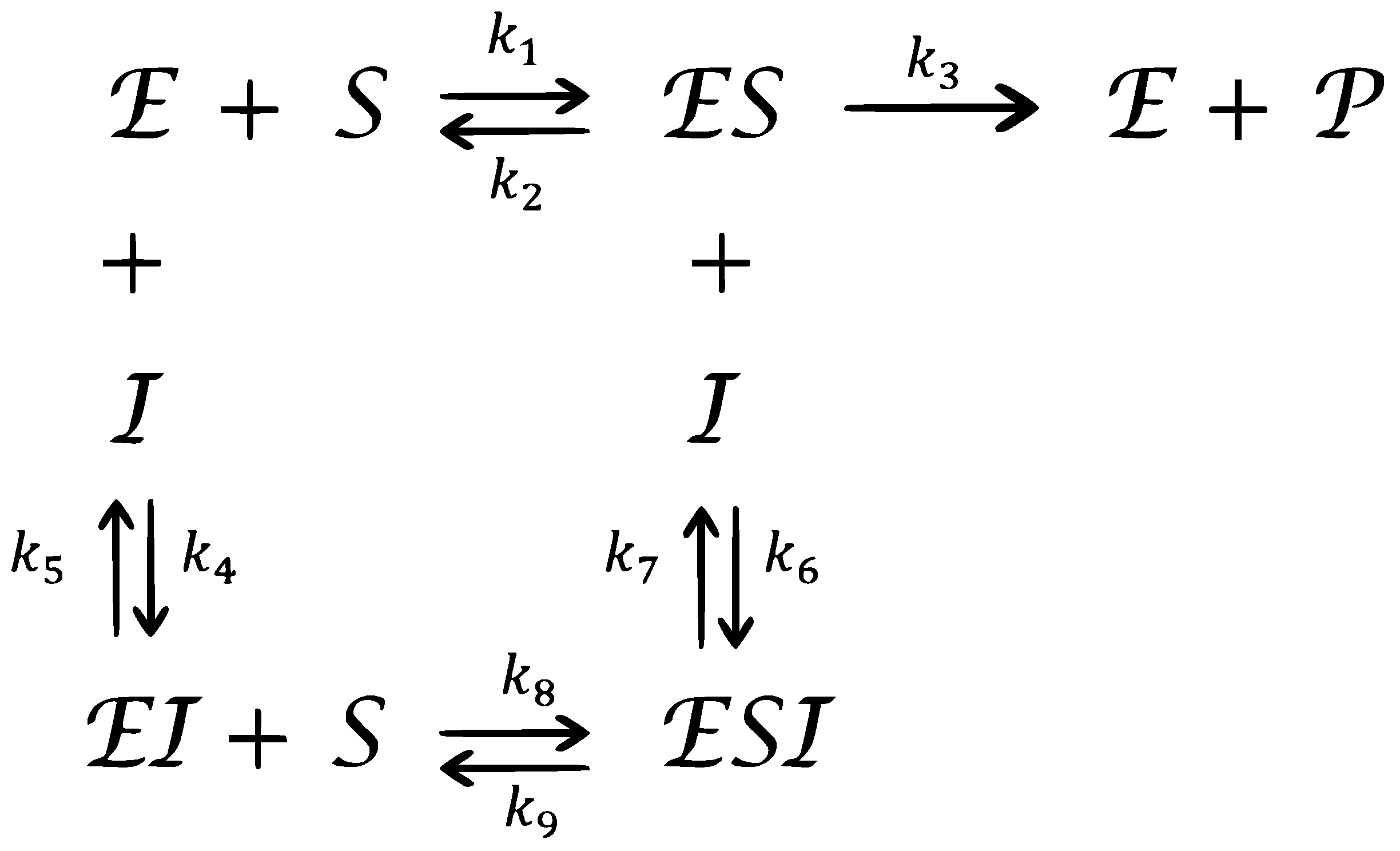
2. A Model of Complex Enzyme Inhibitor Reactions

Consider the complex chemical reaction network for mixed enzymatic inhibition as shown in Figure 1.

Where $\mathcal{E},S,\mathcal{P}$, and $\mathcal{I}$ represent enzyme, substrate, product, and inhibitor, respectively. $\mathcal{E}S,\mathcal{E}I$, and $\mathcal{E}SI$ represent the complex intermediate species. The parameters $k_1,\cdots ,k_9$ represent the rate constants. If we express the concentrations of $\mathcal{E},S,\mathcal{P},\mathcal{I},\mathcal{E}S,\mathcal{E}I$, and $\mathcal{E}SI$ by $E,S,P,I,C_1,C_2$, and $C_3$, respectively, then the mass action law leads to the following nonlinear fractional differential model, which is a modification of the integer-derivative model discussed by Akgül et al. [38]:

$$\begin{array}{c}{D}_t^{\alpha }E=-k_{1}ES+(k_2+k_3)C_1-k_{4}EI+k_5{C}_{2}S,\hfill \\ D_t^{\alpha }S=-k_{1}ES+k_2{C}_1+k_{4}EI-(k_5+k_8)C_{2}S+k_9{C}_3,\hfill \\ D_t^{\alpha }I=-k_{4}EI+k_5{C}_{2}S-k_6{C}_{1}I+k_7{C}_3,\hfill \\ D_t^{\alpha }P=k_3{C}_1,\hfill \\ D_t^{\alpha }{C}_1=k_{1}ES-(k_2+k_3)C_1-k_6{C}_{1}I+k_7{C}_3,\hfill \\ D_t^{\alpha }{C}_2=k_{4}EI-(k_5+k_8)C_{2}S+k_9{C}_3,\hfill \\ D_t^{\alpha }{C}_3=k_6{C}_{1}I-(k_7+k_9)C_3+k_8{C}_{2}S,\hfill \end{array}$$

(1)

where $0<\alpha \le 1$. $D_t^{\alpha }$ is the Caputo fractional derivative defined by

$$D_{x_0}^{\alpha }f\left(x\right)={}^{\mathrm{RL}}{D}_{x_0}^{\alpha }\left(f\left(x\right)-\sum _{k=0}^{m-1}\frac{f^{\left(k\right)}\left(x_0\right)}{k!}{(x-x_0)}^k\right),$$

(2)

where ${}^{\mathrm{RL}}{D}_{x_0}^{\alpha }f\left(x\right)=D^m\left(J_{x_0}^{m-\alpha }f\left(x\right)\right)$, $m-1<\alpha \le m$, and $m\in \mathbb{N}$, and $J_{x_0}^{\alpha }f\left(x\right)$ is the Riemann–Liouville fractional integration of order $\alpha$ for a real-valued function $f:{\mathbb{R}}^{+}\to \mathbb{R}$ defined by

$$J_{x_0}^{\alpha }f\left(x\right)=\frac{1}{\mathsf{\Gamma }\left(\alpha \right)}{\int }_{x_0}^x{(x-s)}^{\alpha -1}f\left(t\right)dt,\alpha >0,x>0.$$

(3)

3. Analytical Expressions for the Concentrations

Consider the nonlinear fractional reaction system (1) subject to the following set of initial concentrations:

$$E\left(0\right)=e_0,S\left(0\right)=s_0,I\left(0\right)=i_0,P\left(0\right)=p_0,C_1\left(0\right)=c_{1_0},C_2\left(0\right)=c_{2_0},C_3\left(0\right)=c_{3_0}.$$

(4)

We will derive two approximate analytical expressions of the concentrations of enzyme, substrate, product, inhibition, and the complex intermediate species using modified Laplace decomposition (LDM) and differential transformation (DTM) methods.

The difference between Riemann–Louivelle and Caputo fractional derivatives, which is just in the order of operators, makes Caputo definition closer to the traditional integer-derivative operator and hence more used than Riemann–Louivelle.

3.1. Laplace Decomposition Approach

We begin with the following lemma whose proof follows immediately from (2) and (3) [39].

Lemma 1.

The Laplace transform of the Caputo fractional derivative of order$\alpha$is given by

$$\mathcal{L}\left\{D^{\alpha }f\left(x\right)\right\}=\frac{s^{m}F\left(s\right)-{\sum }_{i=1}^m{s}^{m-i}{f}^{(i-1)}\left(0\right)}{s^{m-\alpha }},$$

(5)

where$m\in \mathbb{N}$and$m-1<\alpha \le m$.

Applying Laplace transform to each equation in the reaction system (1) gives

$$\begin{array}{c}\mathcal{L}\left\{E\left(t\right)\right\}=\frac{e_0}{s}+\frac{1}{s^{\alpha }}\mathcal{L}\{-k_{1}ES+(k_2+k_3)C_1-k_{4}EI+k_5{C}_{2}S\},\hfill \\ \mathcal{L}\left\{S\left(t\right)\right\}=\frac{s_0}{s}+\frac{1}{s^{\alpha }}\mathcal{L}\{-k_{1}ES+k_2{C}_1+k_{4}EI-(k_5+k_8)C_{2}S+k_9{C}_3\},\hfill \\ \mathcal{L}\left\{I\left(t\right)\right\}=\frac{i_0}{s}+\frac{1}{s^{\alpha }}\mathcal{L}\{-k_{4}EI+k_5{C}_{2}S-k_6{C}_{1}I+k_7{C}_3\},\hfill \\ \mathcal{L}\left\{P\left(t\right)\right\}=\frac{p_0}{s}+\frac{1}{s^{\alpha }}\mathcal{L}\left\{k_3{C}_1\right\},\hfill \\ \mathcal{L}\left\{C_1\left(t\right)\right\}=\frac{{c_1}_0}{s}+\frac{1}{s^{\alpha }}\mathcal{L}\{k_{1}ES-(k_2+k_3)C_1-k_6{C}_{1}I+k_7{C}_3\},\hfill \\ \mathcal{L}\left\{C_2\left(t\right)\right\}=\frac{{c_2}_0}{s}+\frac{1}{s^{\alpha }}\mathcal{L}\{k_{4}EI-(k_5+k_8)C_{2}S+k_9{C}_3\},\hfill \\ \mathcal{L}\left\{C_3\left(t\right)\right\}=\frac{{c_3}_0}{s}+\frac{1}{s^{\alpha }}\mathcal{L}\{k_6{C}_{1}I-(k_7+k_9)C_3+k_8{C}_{2}S\}.\hfill \end{array}$$

(6)

We seek an approximate solution to system (6) and hence a solution to the fractional system (1) in the form of a power series about $t=0$, that is

$$\begin{array}{cc}\hfill & E\left(t\right)=\sum _{n=0}^{\infty }{E}_n\left(t\right),S\left(t\right)=\sum _{n=0}^{\infty }{S}_n\left(t\right),I\left(t\right)=\sum _{n=0}^{\infty }{I}_n\left(t\right),P\left(t\right)=\sum _{n=0}^{\infty }{P}_n\left(t\right),\hfill \\ \hfill & C_1\left(t\right)=\sum _{n=0}^{\infty }{C}_{1_n}\left(t\right),C_2\left(t\right)=\sum _{n=0}^{\infty }{C}_{2_n}\left(t\right),C_3\left(t\right)=\sum _{n=0}^{\infty }{C}_{3_n}\left(t\right).\hfill \end{array}$$

(7)

The nonlinear terms in system (6) are expressed in terms of Adomian polynomials as follows:

$$\begin{array}{cc}\hfill ES& =\sum _{n=0}^{\infty }{A}_{1n}=\frac{1}{n!}{\left(\frac{d}{d\lambda }\right)}^n\left(\sum _{k=0}^n{\lambda }^k{E}_k\sum _{k=0}^n{\lambda }^k{S}_k\right){|}_{\lambda =0},\hfill \\ \hfill EI& =\sum _{n=0}^{\infty }{A}_{2n}=\frac{1}{n!}{\left(\frac{d}{d\lambda }\right)}^n\left(\sum _{k=0}^n{\lambda }^k{E}_k\sum _{k=0}^n{\lambda }^k{I}_k\right){|}_{\lambda =0},\hfill \\ \hfill C_{1}I& =\sum _{n=0}^{\infty }{A}_{3n}=\frac{1}{n!}{\left(\frac{d}{d\lambda }\right)}^n\left(\sum _{k=0}^n{\lambda }^k{\left(C_1\right)}_k\sum _{k=0}^n{\lambda }^k{I}_k\right){|}_{\lambda =0},\hfill \\ \hfill C_{2}S& =\sum _{n=0}^{\infty }{A}_{4n}=\frac{1}{n!}{\left(\frac{d}{d\lambda }\right)}^n\left(\sum _{k=0}^n{\lambda }^k{\left(C_2\right)}_k\sum _{k=0}^n{\lambda }^k{S}_k\right){|}_{\lambda =0}.\hfill \end{array}$$

(8)

Substituting (7) and (8) recursively in (6) and then applying the inverse Laplace transforms lead to the analytical expressions of all concentrations expressed in series forms. The first two terms of each of these series are given below

$$\begin{array}{cc}\hfill & E_0=e_0,S_0=s_0,I_0=i_0,P_0=p_0,C_{1_0}=c_{1_0},C_{2_0}=c_{2_0},C_{3_0}=c_{3_0},\hfill \\ \hfill & E_1=(s_0{c}_{2_0}{k}_5-s_0{e}_0{k}_1+c_{1_0}{k}_2+c_{1_0}{k}_3-i_0{e}_0{k}_4)\frac{t^{\alpha }}{\mathsf{\Gamma }(\alpha +1)},\hfill \\ \hfill & S_1=(-s_0{c}_{2_0}{k}_5-s_0{c}_{2_0}{k}_8-s_0{e}_0{k}_1+c_{1_0}{k}_2-c_{3_0}{k}_9+i_0{e}_0{k}_4)\frac{t^{\alpha }}{\mathsf{\Gamma }(\alpha +1)},\hfill \\ \hfill & I_1=(s_0{c}_{2_0}{k}_5-i_0{c}_{1_0}{k}_6+c_{3_0}{k}_7-i_0{e}_0{k}_4)\frac{t^{\alpha }}{\mathsf{\Gamma }(\alpha +1)},\hfill \\ \hfill & P_1=\left(c_{1_0}{k}_3\right)\frac{t^{\alpha }}{\mathsf{\Gamma }(\alpha +1)},\hfill \\ \hfill & {C_1}_1=(-s_0{e}_0{k}_1-c_{1_0}{k}_2-c_{1_0}{k}_3-i_0{c}_{1_0}{k}_6+c_{3_0}{k}_7)\frac{t^{\alpha }}{\mathsf{\Gamma }(\alpha +1)},\hfill \\ \hfill & {C_2}_1=(-s_0{c}_{2_0}{k}_5-s_0{c}_{2_0}{k}_8+c_{3_0}{k}_9+i_0{e}_0{k}_4)\frac{t^{\alpha }}{\mathsf{\Gamma }(\alpha +1)},\hfill \\ \hfill & {C_3}_1=(s_0{c}_{2_0}{k}_8+i_0{c}_{1_0}{k}_6-c_{3_0}{k}_7-c_{3_0}{k}_9)\frac{t^{\alpha }}{\mathsf{\Gamma }(\alpha +1)}.\hfill \end{array}$$

(9)

3.2. Differential Transformation Method

First proposed by Zhou [40], the differential transformation method (DTM) is an iterative approach for obtaining a Taylor series solution of a differential equation without the need for the tedious computing of symbolic higher derivatives. Arikoglu and Ozkol [41] modified the original version of the DTM to make it applicable to solve fractional differential equations. In this section, we derive a series solution of system (1) using the fractional DTM [42].

The fractional power series expansion of the continuous analytical function $f\left(x\right)$ is given by

$$f\left(t\right)=\sum _{k=0}^{\infty }F\left(k\right){\left(t-t_0\right)}^{k/\alpha },$$

(10)

where $F\left(k\right)$ is the fractional differential transformation of $f\left(t\right)$ defined by

$$F\left(k\right)=\left\{\begin{array}{cc}\frac{1}{(k/\alpha )!}{D}^{k/\alpha }{|}_{t=t_0},\hfill & \mathrm{if}k/\alpha \in Z^{+},k=0,1,2,\dots ,(q\alpha -1)\hfill \\ \\ 0,\hfill & \mathrm{if}k/\alpha \notin Z^{+}\hfill \end{array}\right..$$

(11)

For a fractional-order q, the Caputo fractional derivative is given by

$$D_{t_0}^{q}f\left(t\right)=\frac{1}{\mathsf{\Gamma }(m-q)}{D}^m\left\{{\int }_{t_0}^t\left[\frac{{\displaystyle f\left(t\right)-\sum _{k=0}^{m-1}(1/k!){\left(t-t_0\right)}^k{f}^{\left(k\right)}\left(t_0\right)}}{{(t-x)}^{1+q-m}}\right]\mathrm{d}t\right\}.$$

(12)

The following properties of fractional differential transformations are needed in the derivation of the analytical solution of system (1) [42].

Theorem 1.

If$f\left(x\right)=g_1\left(x\right)\pm g_2\left(x\right)\pm \cdots \pm g_n\left(x\right)$, then$F\left(k\right)=G_1\left(k\right)\pm G_2\left(k\right)\pm \cdots \pm G_n\left(k\right).$

Theorem 2.

If${\displaystyle f\left(x\right)=\prod _{j=1}^n{g}_j\left(x\right)}$, then

${\displaystyle F\left(k\right)=\sum _{k_{n-1}=0}^k\sum _{k_{n-2}=0}^{k_{n-1}}\cdots \sum _{k_2=0}^{k_3}\sum _{k_1=0}^{k_2}{G}_1\left(k_1\right)G_2\left(k_2-k_1\right)\dots G_{n-1}\left(k_{n-1}-k_{n-2}\right)G_n\left(k-k_{n-1}\right).}$

Theorem 3.

If$f\left(x\right)={\left(x-x_0\right)}^p$, then$F\left(k\right)=\delta (k-\alpha p)$, where

$\delta \left(k\right)=\left\{\begin{array}{cc}1\hfill & ifk=0\hfill \\ 0\hfill & ifk\ne 0\hfill \end{array}\right..$

Theorem 4.

If$f\left(x\right)=D_{x_0}^q\left[g\left(x\right)\right]$, then${\displaystyle F\left(k\right)=\frac{\mathsf{\Gamma }(q+1+k/\alpha )}{T(1+k/\alpha )}G(k+\alpha q).}$

By applying the fractional operator in (12) to system (1), we obtain the same series solution given in (10) for the integer case. For fractional order derivatives, the variations between the LDM and DTM were very small, and will be discussed in the Results and Discussion section.

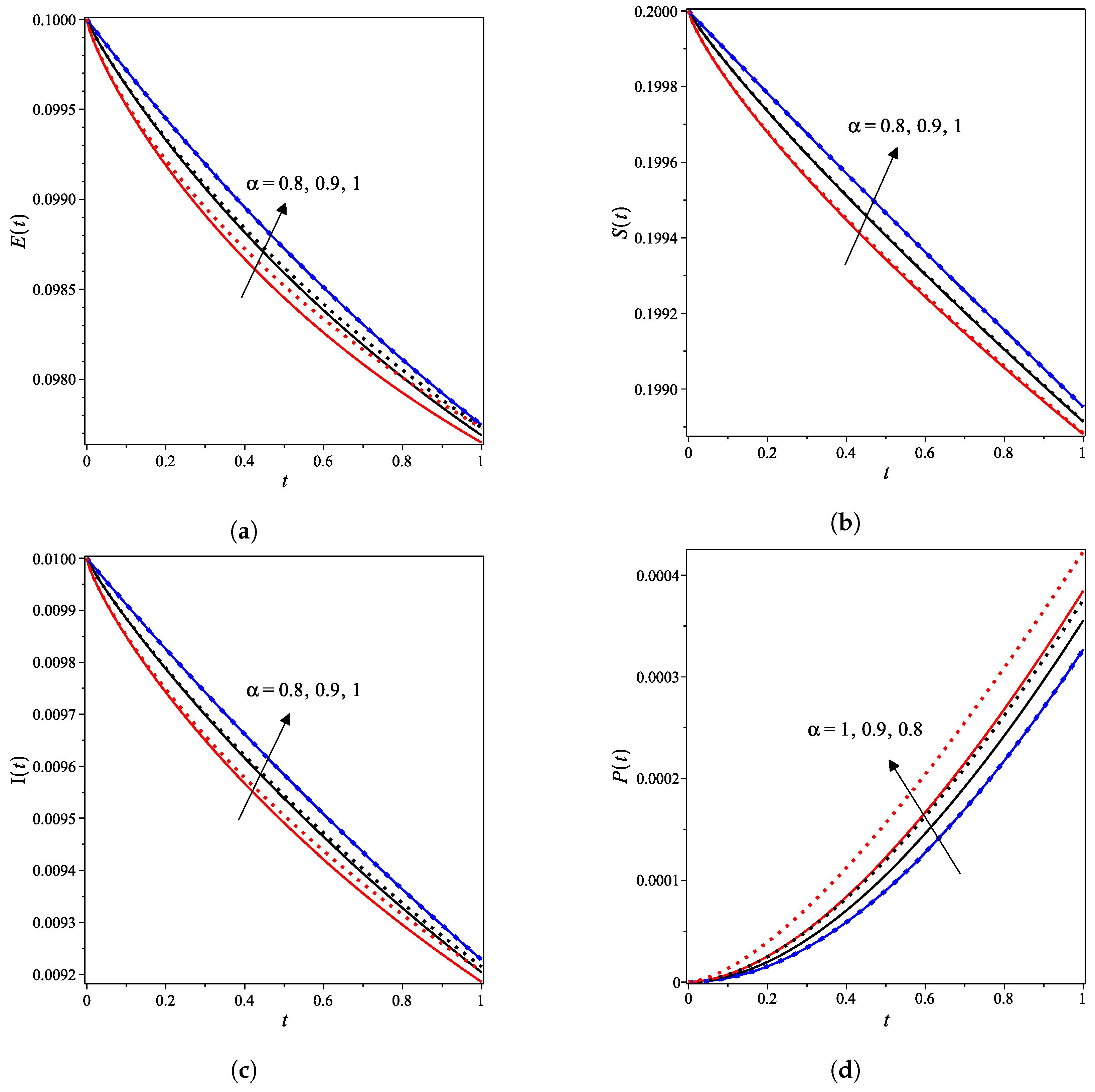
3.3. Padé Approximation

It is known that the convergence of the truncated series solutions obtained by Laplace decomposition and differential transformation methods are guaranteed only over small domains. The divergence of the series solution obtained by the LDM or DTM may also result for large initial conditions. In this case, LDM and DTM methods can be coupled with Padé approximation to insure convergence. The Padé approximant of the function $f\left(x\right)$, which is a convergent ratio of two polynomials constructed from its Taylor series expansion, gives a better approximation of the function, especially when there are poles.

When the function $f\left(x\right)$ is expressed as a power series, the $[L/M]$ Padé approximant is given by

$$f\left(x\right)=\frac{P_L\left(x\right)}{Q_M\left(x\right)}=\frac{p_0+p_{1}x+p_2{x}^2+p_3{x}^3+\cdots +p_L{x}^L}{1+q_{1}x+q_2{x}^2+q_3{x}^3+\cdots +q_M{x}^M}.$$

(13)

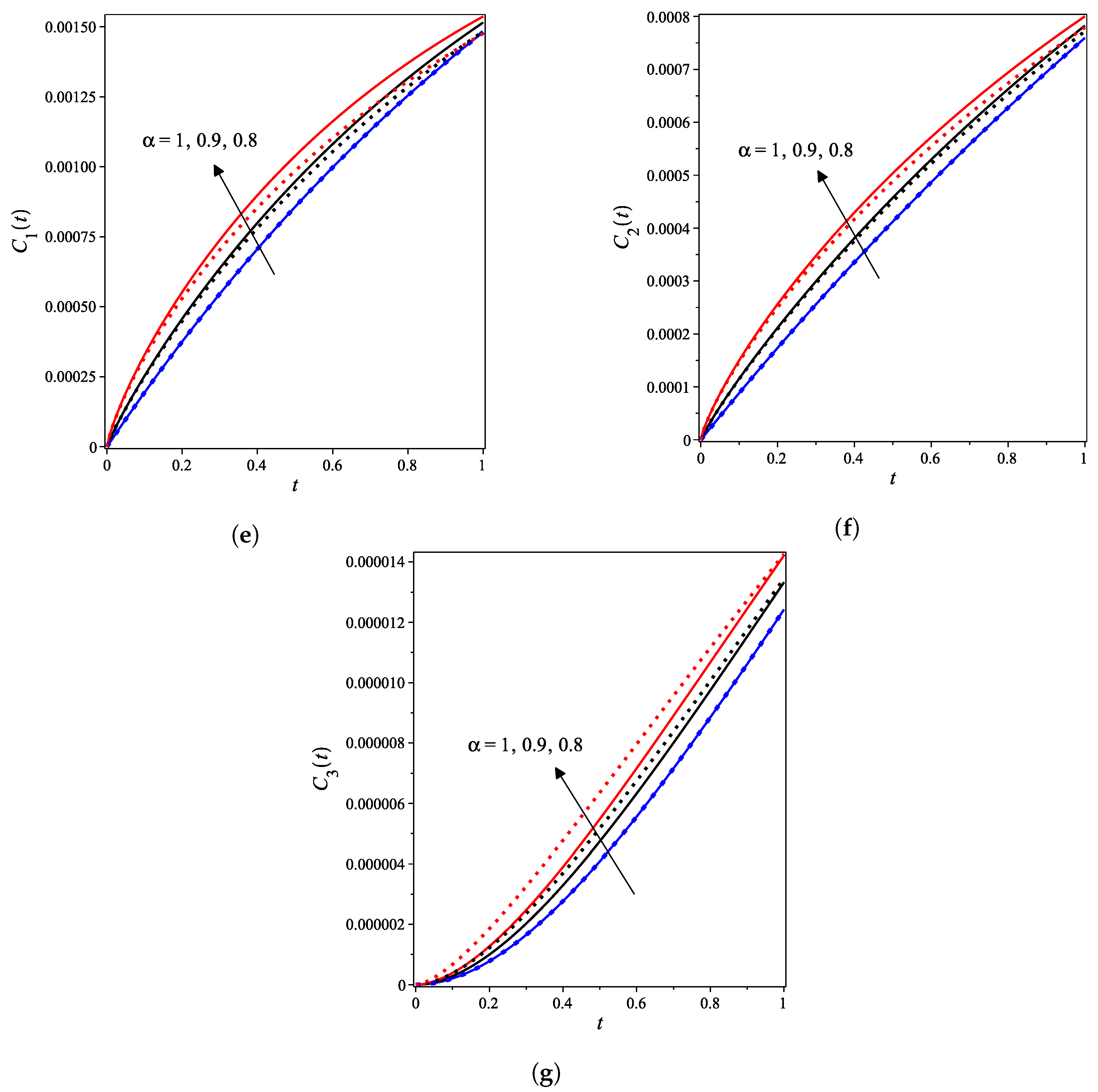
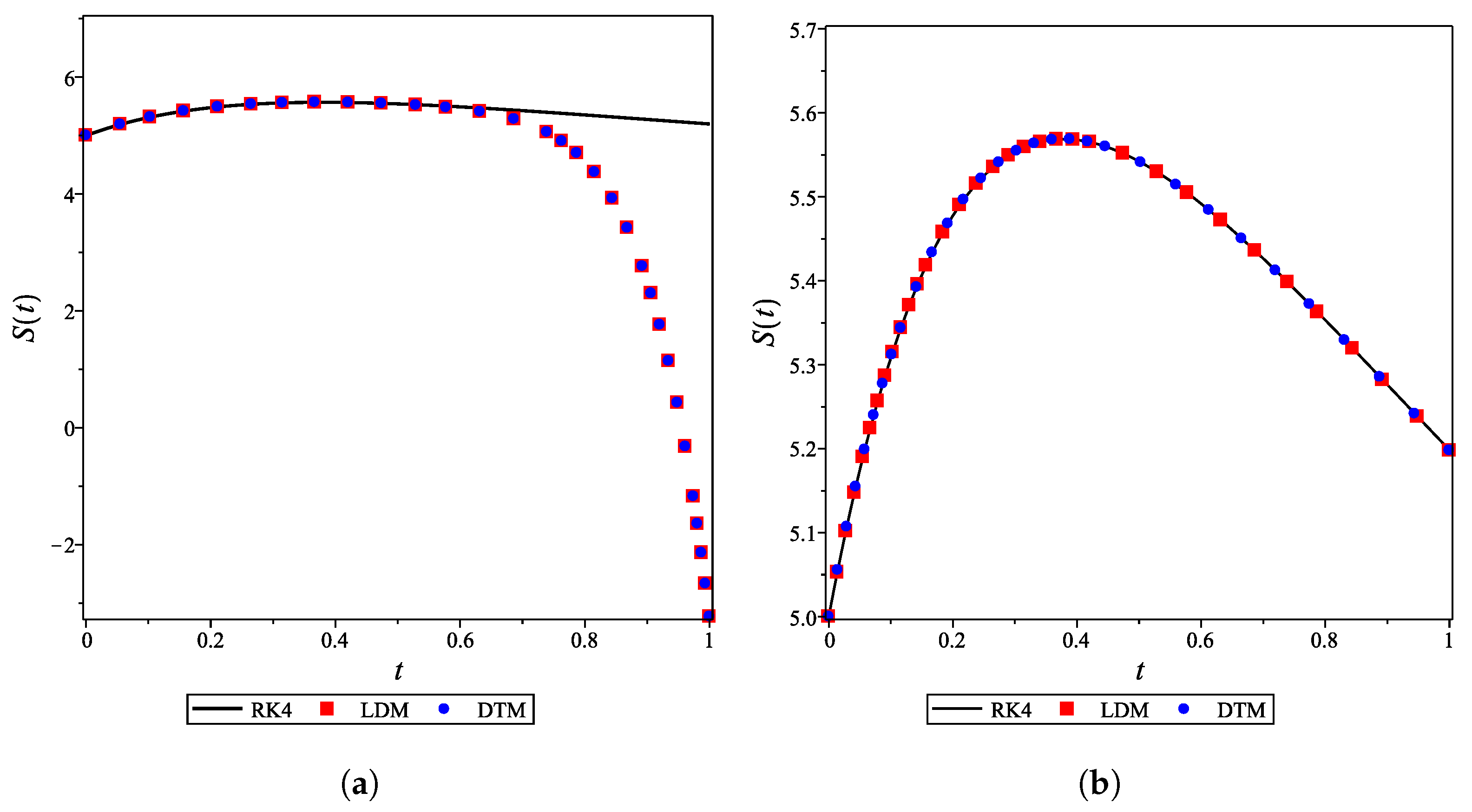
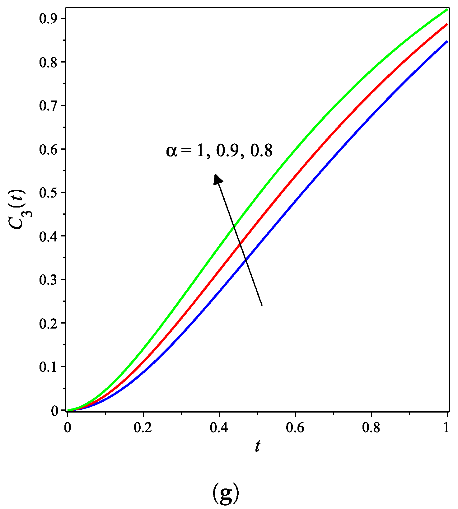
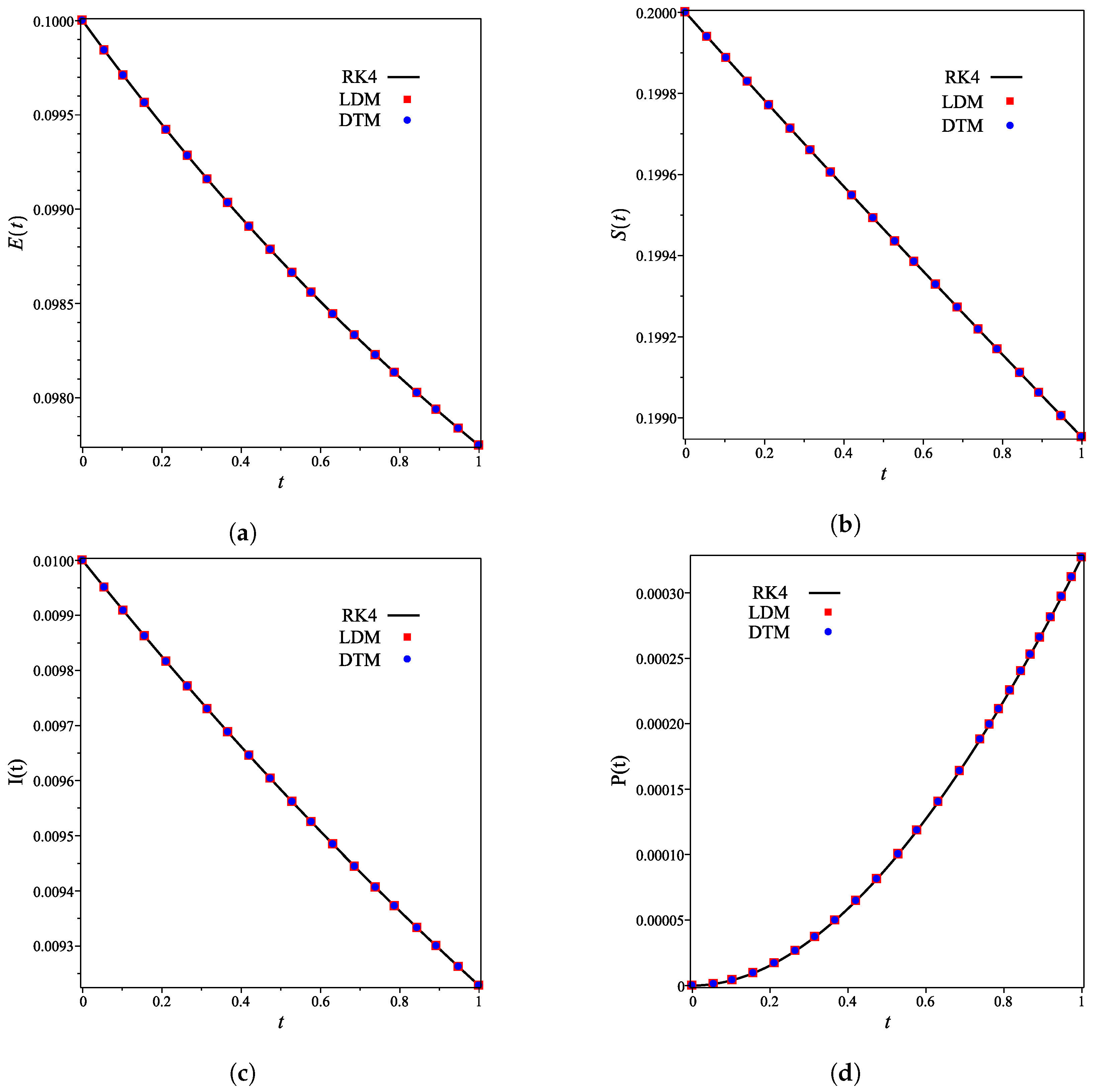
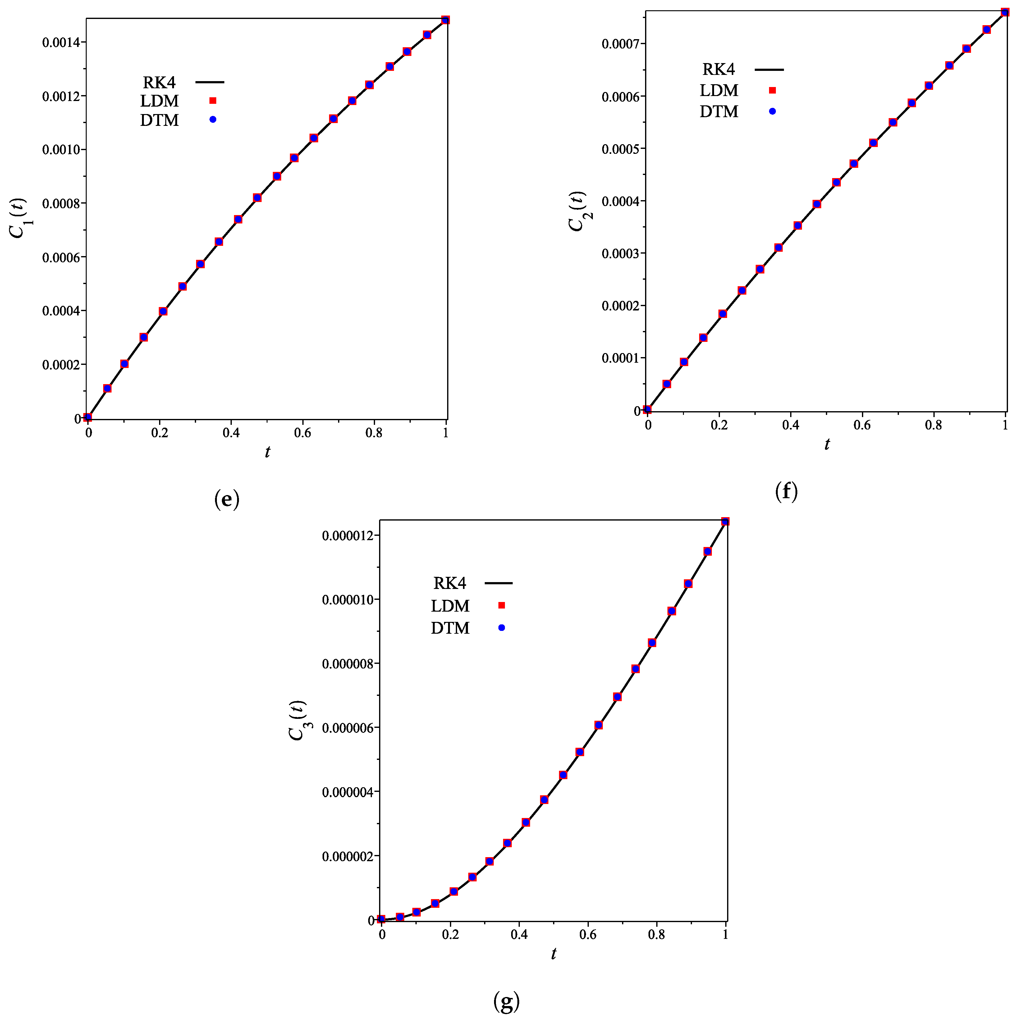
4. Results and Discussion

In this section, two study cases are presented. In each case, the nonlinear reaction system (1) is solved for a different set of parameters and a different set of initial concentrations.

Example 1.

To verify the accuracy of the proposed approaches, we first solve the underlined system for the integer-derivative, $\alpha =1$, subject to the following initial conditions (4).

$$e_0=0.1,s_0=0.2,i_0=0.01,p_0={c_1}_0={c_2}_0={c_3}_0=0,$$

(14)

and the following constant rates

$$k_1=0.1,k_2=0.2,k_3=0.4,k_4=0.9,k_5=1,k_6=0.4,k_7=0.9,k_8=0.2,k_9=0.5.$$

(15)

The LDM and DTM solutions were identical for all seven species. For example, the identical five-term series solution obtained by the LDM and the DTM representing the concentration of enzyme is given by

$$E\left(t\right)=0.1-0.0029t+0.000778t^2-0.000152t^3+0.0000242t^4.$$

(16)

The analytical expressions of the concentrations of all other species are provided in the Supporting Information. Figure 2a–g shows that for the integer case ($\alpha =1$), the derived analytical concentration curves obtained by the LDM and the DTM are identical and strongly agree with the fourth-order Runge–Kutta numerical curves. Figure 2 also reflects the temporal dependence of relative concentrations of enzyme reaction components. It is noticed that concentrations of enzyme, substrate, and product decrease as time increases, whereas the concentrations of inhibitor, enzyme–substrate, enzyme–inhibitor, and enzyme–substrate–inhibitor increase with time.

The nonlinear fractional reaction system (1) is also solved for the fractional derivatives $\alpha =0.9,$ and $\alpha =0.8$. Figure 3a–g shows strong agreements between LDM and DTM concentration curves of enzyme, substrate, product, inhibition and all complex intermediate species. In this Figure, the fractional derivative $\alpha$ is an index of memory, where it is noticed that the concentrations of the enzyme components depend on the fractional order. Figure 3 clearly shows that as $\alpha$ increases, the fractional concentration curve gets closer to the curve representing the concentration for the integer case ($\alpha =1$).

Figure 3a–c confirms that the enzyme, substrate, and inhibitor concentrations increase as the fractional power increases and decrease as time increases. In contrast, Figure 3d–g portrays that the product and intermediate species concentrations increase and reach their maximum with the rise of time and decrease of the fractional power.

Table 1. Maximum variation between LDM and DTM computed concentrations when $\alpha =0.9$.

Concentration	Maximum Difference	Occurred at x
Enzyme	0.0000424	1.000
Substrate	0.0000024	0.007
Inhibition	0.0000103	1.000
Production	0.0000205	0.925
Complex ES	0.0000323	0.925
Complex EI	0.0000105	1.000
Complex ESI	0.0000004	0.525

and

Table 2. Maximum variation between LDM and DTM computed concentrations when $\alpha =0.8$.

Concentration	Maximum Difference	Occurred at x
Enzyme	0.0000843	0.850
Substrate	0.0000049	0.600
Inhibition	0.0000206	1.000
Production	0.0000408	0.825
Complex ES	0.0000643	0.825
Complex EI	0.0000208	1.950
Complex ESI	0.0000009	0.450

assert that the actual variations between the LDM and DTM for the fractional cases are smaller than what they appear in Figure 3. This can also be inferred from the very small y-axis increments in Figure 3.

Example 2.

Consider the nonlinear fractional reaction system (1) subject to the following set of relatively large initial concentrations:

$$e_0=12,s_0=5,i_0=2,p_0={c_1}_0={c_2}_0={c_3}_0=0,$$

(17)

and the following set of constant rates

$$k_1=0.01,k_2=0.2,k_3=0.04,k_4=0.19,k_5=0.1,k_6=0.4,k_7=0.09,k_8=0.22,k_9=0.05.$$

(18)

For the integer case, $\alpha =1$, the obtained LDM, and DTM truncated series solutions (concentrations) were identical but diverged rapidly over a small domain. This divergence was controlled by using a $[4/4]$ Padé approximant for each analytical derived expression. In Figure 4a, the divergent enzyme concentration curves obtained by the LDM and DTM are depicted against time. In contrast, Figure 4b shows how the use of Padé approximation overcomes this obstacle. Figure 5 is similar to Figure 4 but for the substrate concentration. All concentration curves for the case $\alpha =1$ and their $[4/4]$ corresponding Padé approximations are provided in the Supporting Information.

The DTM was employed to derive analytical expressions for the concentration curves of all species for fractional values of $\alpha$ ($\alpha =0.9,0.8$). All the obtained curves of more than 10-term truncated series (provided in the Supporting Information) diverged over a relatively small domain. Therefore, large order Padé approximations were needed to obtain the convergent series solutions, as shown in Figure 6. A single command using Maple or MATLAB can be used to generate Padé approximations (given in supplementary material).

5. Conclusions

This paper discussed a complex nonlinear fractional model of enzyme inhibitor reactions subject to two different sets of initial concentrations, each with a different set of reaction rates. The simple, efficient, and reliable Laplace decomposition (LDM) and differential transformation (DTM) methods were utilized to solve the nonlinear fractional biochemical reaction system. The LDM was implemented by using Laplace transform of Caputo fractional derivative to convert the nonlinear fractional-derivative system (1) into an algebraic system, where the nonlinear terms are expressed in the form of Adomian polynomials. Then, the solution is obtained by employing the linearity of the Laplace and the inverse Laplace transforms. The fractional differential transformation method was implemented by directly applying Equations (10) and (11), and Theorem 2. The derived solution of system (1) represent the analytic expressions for the concentrations of enzyme, inhibitor, substrate, product, and the complex intermediate species: enzyme–substrate, enzyme–inhibitor, and enzyme–inhibitor–substrate were derived and discussed. From this study, it was concluded that different rate constants and initial concentrations produce different dynamics. Furthermore, it was shown that a Padé approximation of the series solution obtained by LDM and DTM would preserve convergence and stability when large initial concentrations or large rate constants are assumed. The derived LDM and DTM concentration expressions for the enzyme inhibitor reaction model were shown to be very close to the fourth-order Runge–Kutta method when the results were compared for the integer-derivative case.

The derived fractional analytical concentration curves would play a significant role in predicting the future state of the biochemical reaction model. In addition, the derived analytical expressions would be essential in investigating the effects of various reaction rates to reach better designs and controlled systems. The used methods are accessible to the broader research community. They can be extended to solve various fractional models to obtain a better insight into dynamical behavior for biological or chemical systems with possible hereditary properties.

References

1. Saravanakumar, R.; Pirabaharan, P.; Abukhaled, M.; Rajendran, L. Theoretical analysis of voltammetry at a rotating disk electrode in the absence of supporting electrolyte. J. Phys. Chem. B 2020, 124, 443–450. [Google Scholar] [CrossRef]
2. Abukhaled, M.; Guessoum, N.; Alsaeed, N. Mathematical modeling of light curves of RHESSI and AGILE terrestrial gamma-ray flashes. Astrophys. Space Sci. 2019, 364, 120. [Google Scholar] [CrossRef]
3. Saravanakumar, S.; Eswari, A.; Rajendran, L.; Abukhaled, M. A mathematical model of risk factors in HIV/AIDS transmission Dynamics: Observational study of female sexual network in India. Appl. Math. Inf. Sci. 2020, 14, 967–976. [Google Scholar]
4. Devi, M.C.; Pirabaharan, P.; Abukhaled, M.; Rajendran, L. Analysis of the steady-state behavior of pseudo-first-order EC-catalytic mechanism at a rotating disk electrode. Electrochim. Acta 2020, 345, 136175. [Google Scholar] [CrossRef]
5. Abukhaled, M.; Khuri, S. An efficient semi-analytical solution of a one-dimensional curvature equation that describes the human corneal shape. Math. Comput. Appl. 2019, 24, 8. [Google Scholar] [CrossRef] [Green Version]
6. Selvi, M.S.M.; Rajendran, L.; Abukhaled, M. Estimation of Rolling Motion of Ship in Random Beam Seas by Efficient Analytical and Numerical Approaches. J. Mar. Sci. Appl. 2021, 20, 55–66. [Google Scholar] [CrossRef]
7. Patnaik, S.; Hollkamp, J.P.; Semperlotti, F. Applications of variable-order fractional operators: A review. Proc. R. Soc. A 2020, 476, 20190498. [Google Scholar] [CrossRef] [Green Version]
8. Flores-Tlacuahuac, A.; Biegler, L. Optimization of Fractional Order Dynamic Chemical Processing Systems. Ind. Eng. Chem. Res. 2014, 53, 5110–5127. [Google Scholar] [CrossRef]
9. Ionescu, C.; Lopes, A.; Copot, D.; Machado, J.; Bates, J. The role of fractional calculus in modeling biological phenomena: A review. Commun. Nonlinear. Sci. Numer. Simulat. 2017, 51, 141–159. [Google Scholar] [CrossRef]
10. Rihan, F.A. Numerical modeling of fractional-order biological systems. Abstr. Appl. Anal. 2013, 2013, 816803. [Google Scholar] [CrossRef] [Green Version]
11. Lazopoulos, K.A.; Lazopoulos, A.K. Fractional vector calculus and fluid mechanics. J. Mech. Behav. Biomed. Mater. 2017, 26, 43–54. [Google Scholar] [CrossRef]
12. Gomez-Aguilar, J.F.; Cordova-Fraga, T.; Escalante-Martínez, J.E.; Calderon-Ram, C.; Escobar-Jimenez, R.F. Electrical circuits described by a fractional derivative with regular Kernel. Rev. Mex. De Fis. 2016, 62, 144–154. [Google Scholar]
13. Meral, F.C.; Royston, T.J.; Magin, R. Fractional calculus in viscoelasticity: An experimental study. Ommun. Nonlinear. Sci. Numer. Simulat. 2010, 15, 939–945. [Google Scholar] [CrossRef]
14. Matušů, R. Application of fractional order calculus to control theory. Math Model. Methods Appl. Sci. 2011, 5, 1162–1169. [Google Scholar]
15. Srivastava, H.M. Fractional-order derivatives and integrals: Introductory overview and recent developments. Kyungpook Math. J. 2020, 60, 73–116. [Google Scholar]
16. Dubey, V.P.; Kumar, R.; Kumar, D. Approximate analytical solution of fractional order biochemical reaction model and its stability analysis. Int. J. Biomath. 2019, 12, 1950059. [Google Scholar] [CrossRef]
17. Dulf, E.-H.; Vodnar, D.C.; Danku, A.; Muresan, C.; Crisan, O. Fractional-Order Models for Biochemical Processes. Fractal Fract. 2020, 4, 12. [Google Scholar] [CrossRef] [Green Version]
18. Iyiola, O.; Tasbozan, O.; Kurt, A.; Çenesiz, Y. On the analytical solutions of the system of conformable time-fractional Robertson equations with 1-D diffusion. Chaos Solitons Fractals 2017, 94, 1–7. [Google Scholar] [CrossRef]
19. Arafa, A. Different approach for conformable fractional biochemical reaction diffusion models. Appl. Math. J. Chin. Univ. 2020, 35, 452. [Google Scholar] [CrossRef]
20. Baeumer, B.; Kovacs, M.; Meerschaert, M. Numerical solutions for fractional reaction diffusion equations. Comput. Math. Appl. 2008, 55, 2212. [Google Scholar] [CrossRef] [Green Version]
21. Atangana, A. Modeling the Enzyme Kinetic Reaction. Acta Biotheor 2015, 63, 239. [Google Scholar] [CrossRef] [PubMed]
22. Bhrawy, A.; Zaky, M. Numerical simulation for two-dimensional variable-order fractional nonlinear cable equation. Nonlinear Dyn. 2015, 80, 101–116. [Google Scholar] [CrossRef]
23. Atangana, A.; Owolabi, K.M. New numerical approach for fractional differential equations. Math. Model. Nat. Phenom. 2018, 13, 3. [Google Scholar] [CrossRef] [Green Version]
24. Milici, C.; Machado, J.T. Draganescu, G. Application of the Euler and Runge–Kutta Generalized Methods for FDE and Symbolic Packages in the Analysis of Some Fractional Attractors. Int. J. Nonlinear Sci. Numer. Simul. 2020, 21, 159–170. [Google Scholar] [CrossRef]
25. Jhinga, A.; Daftardar-Gejji, V. A new numerical method for solving fractional delay differential equations. Comput. Appl. Math. 2019, 38, 166. [Google Scholar] [CrossRef]
26. Kumar, S.; Baleanu, D. A new numerical method for time fractional non-linear sharma-tasso-oliver equation and klein-gordon equation with exponential kernel law. Front. Phys. 2020, 8, 136. [Google Scholar] [CrossRef]
27. Ali, U.; Khan, M.A.; Khater, M.M.A.; Mousa, A.A.; Attia, R.A.M. A new numerical approach for solving 1D fractional diffusion-wave equation. J. Funct. Spaces 2021, 2021, 1–7. [Google Scholar] [CrossRef]
28. Toufik, M.; Atangana, A. New numerical approximation of fractional derivative with non-local and non-singular kernel: Application to chaotic models. Eur. Phys. J. Plus 2017, 132, 444. [Google Scholar] [CrossRef]
29. Devi, M.C.; Pirabaharan, P.; Rajendran, L.; Abukhaled, M. An efficient method for finding analytical expressions of substrate concentrations for different particles in an immobilized enzyme system. Reac. Kinet. Mech. Cat. 2020, 130, 35–53. [Google Scholar] [CrossRef]
30. Javeed, S.; Baleanu, D.; Waheed, A.; Shaukat, K.M.; Affan, H. Analysis of Homotopy Perturbation Method for Solving Fractional Order Differential Equations. Mathematics 2019, 7, 40. [Google Scholar] [CrossRef] [Green Version]
31. Zurigat, M.; Momani, S.; Odibat, Z.; Alawneh, A. The homotopy analysis method for handling systems of fractional differential equations. Appl. Math. Model. 2010, 34, 24–35. [Google Scholar] [CrossRef]
32. Mohammed, O.; Salim, H. Computational methods based laplace decomposition for solving nonlinear system of fractional order differential equations. Alex. Eng. J. 2018, 57, 3549–3557. [Google Scholar] [CrossRef]
33. He, C.-H.; Shen, Y.; Ji, F.-Y.; He, J.-H. Taylor series solution for fractal Bratu-type equation arising in electrospinning process. Fractals 2020, 28, 2050011. [Google Scholar] [CrossRef]
34. Hadid, S.; Khuri, S.A.; Sayfy, A. A Green’s function iterative approach for the solution of a class of fractional BVPs arising in physical models. Int. J. Appl. Comput. Math. 2020, 6, 91. [Google Scholar] [CrossRef]
35. Morales-Delgado, V.F.; Gomez-Aguilar, J.F.; Saad, K.; Khan, M.; Agarwal, P. Analytic solution for oxygen diffusion from capillary to tissues involving external force effects: A fractional calculus approach. Phys. A: Stat. Mech. Appl. 2019, 523, 48–65. [Google Scholar] [CrossRef]
36. Abukhaled, M.; Khuri, S.; Rabah, F. Solution of a nonlinear fractional COVID-19 model. Int. J. Numer. Methods Heat Fluid Flow 2022. ahead-of-print. [Google Scholar] [CrossRef]
37. Ganjefar, S.; Rezaei, S. Modified homotopy perturbation method for optimal control problems using the Padé approximant. Appl. Math. Model. 2016, 40, 7062–7081. [Google Scholar] [CrossRef]
38. Akgül, A.; Khoshnaw, S.H. Application of fractional derivative on non-linear biochemical reaction models. Int. J. Intell. Netw. 2020, 1, 52–58. [Google Scholar] [CrossRef]
39. Alchikh, R.; Khuri, S.A. Numerical solution of a fractional differential equation arising in optics. Optik 2020, 208, 163911. [Google Scholar] [CrossRef]
40. Zhou, J.K. Differential Transformation and Its Applications for Electrical Circuits; Huazhong University Press: Wuhan, China, 1986. [Google Scholar]
41. Arikoglu, A.; Ozkol, I. Solution of fractional differential equations by using differential transform method. Chaos Solitons Fractals 2007, 34, 1473–1481. [Google Scholar] [CrossRef]
42. Ertürk, V.S.; Momani, S. Solving systems of fractional differential equations using differential transform method. J. Comput. Appl. Math. 2008, 215, 142–151. [Google Scholar] [CrossRef] [Green Version]
Figure 1. A complex chemical reaction for a mixed enzymatic inhibition.
Mca 27 00045 g001
Figure 2. Analytical and numerical concentration curves for reaction system (1) for the integer-derivative case ( α = 1 ) with initial concentrations (14) and rate constants (15). (a) Enzyme. (b) Substrate. (c) Product. (d) Inhibitor. (e) Intermediate species ES. (f) Intermediate species EI. (g) Intermediate species ESI.
Mca 27 00045 g002aMca 27 00045 g002b
Figure 3. Analytical concentration curves for fractional reaction system (1) with initial concentrations (14) and rate constants (15) for the integer-derivative case α = 1 and the fractional-derivative cases α = 0.9 and 0.8 . Solid and dotted curves represent the LDM and the DTM solutions, respectively. (a) Enzyme. (b) Substrate. (c) Product. (d) Inhibitor. (e) Intermediate species ES. (f) Intermediate species EI. (g) Intermediate species ESI.
Mca 27 00045 g003aMca 27 00045 g003b
Figure 4. Analytical and numerical concentration curves of Enzyme ( E ( t ) ) for the integer-derivative system (1) with α = 1 , initial conditions (17), and parameters (18). (a) Divergent analytical concentration curve. (b) Convergent analytical concentration curve.
Mca 27 00045 g004
Figure 5. Analytical and numerical concentration curves of substrate ( S ( t ) ) for integer-derivative system (1) with α = 1 , initial conditions (17), and parameters (18). (a) Divergent analytical concentration curve. (b) Convergent analytical concentration curve.
Mca 27 00045 g005
Figure 6. Analytical LDM concentration curves of E , S , I , P , E S , E I and E S I for system (1) with initial conditions (17) and parameters (18). (a) Enzyme. (b) Substrate. (c) Product. (d) Inhibitor. (e) Intermediate species ES. (f) Intermediate species EI. (g) Intermediate species ESI.
Mca 27 00045 g006aMca 27 00045 g006b