Characterization of the Vibration and Strain Energy Density of a Nanobeam under Two-Temperature Generalized Thermoelasticity with Fractional-Order Strain Theory

Abstract

In this work, fractional-order strain theory was applied to construct a novel model that introduces a thermal analysis of a thermoelastic, isotropic, and homogeneous nanobeam. Under supported conditions of fixed aspect ratios, a two-temperature generalized thermoelasticity theory based on one relaxation time was used. The governing differential equations were solved using the Laplace transform, and their inversions were found by applying the Tzou technique. The numerical solutions and results for a thermoelastic rectangular silicon nitride nanobeam were validated and supported in the case of ramp-type heating. Graphs were used to present the numerical results. The two-temperature model parameter, beam size, ramp-type heat, and beam thickness all have a substantial influence on all of the investigated functions. Moreover, the parameter of the ramp-type heat might be beneficial for controlling the damping of nanobeam energy.

1. Introduction

The mixed heat thermoelasticity principle is composed of two different partial differential equations: the energy conservation equation and the mechanical equation, both of which are based on the Fourier fundamental theorem [1]. By adding the concept of relaxation time for an isotropic body, Lord and Shulman (L-S) have modified and updated the classical Fourier heat conduction rule [2]. Cattaneo’s rule of heat conduction was developed to change the classic Fourier law by including the heat flow and its time scale shift. In this context, the heat conduction equation is the hyperbolic differential equation. The issue with infinite transmission rates has now been eliminated [3,4,5,6,7].

The nanobeam’s vibration is the most critical of micro/nanobeam resonators. Sharma and Grover investigated the transverse vibrations of thin beam resonators with isotropic, homogenous, and thermoelastic voids [8]. Sun and Saka formulated the thermoelastic damping vibrations of circular plate resonators using out-of-plane microplates [9]. They included a component in their thermoelastic damping formula that is not included in Lifshitz and Roukes’s formula and is based on Poisson’s ratio [10].

Numerous researchers have examined the vibrational and thermal transmission mechanisms of nanobeams [11,12,13,14,15]. The vibration of a gold nanobeam subjected to a thermal shock has been studied by Al-Lehaibi and Youssef [12]. By applying the characteristics of the Green functions, Kidawa investigated the impact of internal and exterior damping of nanobeam vibration due to a heat source moving at a constant speed [14]. The vibrations of a simply supported rectangular nanobeam exposed to a certain thermal shock spread throughout its length have been investigated by Boley [13].

Manolis and Beskos investigated nanobeam systems’ mediated vibration. They utilized a computer technique to study the thermoelastic dynamic reaction of the nanobeam structure to thermomechanical stress [15]. Al-Huniti et al. have studied the thermal response that caused movement and pressures on the heated rod due to a fast-moving laser beam, as well as the dynamic actions of the heated rod from using Laplace equations [11].

Youssef tested, using two different temperatures, the concept of universal two-temperature thermoelasticity. He developed principles of dynamic and conductive temperatures, where the difference between them is related to the material’s heat supply [16].

The first paradigm was examined by Magin and Royston using a version of a fractional strain sequence that describes the materials’ nature and is based on the definition of the fraction’s calculus. If the derivative order is zero, we use the Hookean solid state to obtain the Newtonian stream. Elastic and viscoelastic components were in the range of zero to one [17]. Tissue cartilage practice demonstrates a diverse architecture ranging from independent collagen to twisted macromolecular fiber families and a network of connective living tissue cells. The greatest challenge for bioengineering is estimating the macro-mechanical properties of cartilage using a multi-scale model based on the current concept [17]. A new theorem of generalized thermoelasticity based on the definition of fractional-order strain was established by Youssef and used for the first known problem in thermoelasticity [18].

Thus, this work introduces thermal analysis for a thermoelastic, isotropic, and homogenous nanobeam within the theory of fractional-order strain in the context of the generalized two-temperature thermoelasticity model with one relaxation time theory. The numerical results for a thermoelastic rectangular nanobeam of silicon nitride were validated in the case of ramp-type heating and simple support.

2. Basic Equations

In the Cartesian coordinate system, we consider an isotropic, regular, thermally conducting, and thermoelastic beam. Initially, at a reference temperature $T_0$ and rest, it is undeformed. The equivalent differential values were developed based on the principle of fractional stress order in the sense of the standard two-temperature thermoelasticity and non-Fourier thermal control law. The displacement vector is defined as $U=\left(u,v,w\right)$, and $T^d$ denotes the absolute dynamical temperature, while $T^C$ denotes the absolute conductive temperature. Moreover, no external body forces or heat sources have been assumed. Thus, the governing equations are given by [19]:

The motion equations take the form:

$${\sigma }_{ij,j}=\rho {\ddot{U}}_{i}i,j=1,2,3$$

(1)

The constitutive equations of stress–strain based on fractional-order strain take the forms [18,20,21]:

$${\sigma }_{ij}=\left(1+{\tau }^{\beta }{D}_t^{\beta }\right)\left(2\mu e_{ij}+\lambda e_{kk}{\delta }_{ij}\right)-\gamma \left(1+{\tau }^{\beta }{D}_t^{\beta }\right)\theta {\delta }_{ij}i,j=1,2,3$$

(2)

The two-temperature heat conduction equations take the forms [18]:

$$K{\phi }_{,ii}=\rho C_{\upsilon }\left(\frac{\partial }{\partial t}+{\tau }_0\frac{{\partial }^2}{\partial t^2}\right)\theta +\gamma T_0\left(1+{\tau }^{\beta }{D}_t^{\beta }\right)\left(\frac{\partial }{\partial t}+{\tau }_0\frac{{\partial }^2}{\partial t^2}\right)e_{ij}{\delta }_{ij}i,j=1,2,3$$

(3)

and

$$\theta =\phi -a{\phi }_{,ii}i=1,2,3$$

(4)

The strains (strains) are in the form:

$$2e_{ij}=\left(U_{i,j}+U_{j,i}\right)i,j=1,2,3$$

(5)

where $\phi =T^c-T_0$ is the heat conduction increment, $\theta =T^d-T_0$ defines the dynamical temperature increment, $a\ge 0$ is called the two-temperature parameter, $i,j=x,y,z$, $\gamma =\left(3\lambda +2\mu \right){\alpha }_T$, ${\alpha }_T$ is the linear thermal expansion coefficient, $\rho$ denotes the density, $\lambda ,\mu$ are Lamè’s parameters, ${\delta }_{ij}$ is the Kronecker delta symbol, ${\tau }_0$ defines the thermal relaxation time, $\tau$ denotes the mechanical relaxation time parameter, and $C_{\upsilon }$ is the specific heat at a constant strain.

The fractional derivative concerning the time $D_t^{\beta }$ is defined as [16,18]:

$$D_t^{\beta }f\left(t\right)=\left\{\begin{array}{cc}\frac{1}{\mathsf{\Gamma }\left(1-\beta \right)}{\displaystyle \underset{0}{\overset{t}{\int }}\frac{f^{\prime }\left(\xi \right)}{{\left(t-\xi \right)}^{\beta }}}d\xi & 0\le \beta <1\\ \frac{\partial f\left(t\right)}{\partial t}& \beta =1\end{array}\right\}$$

(6)

3. Problem Formulation

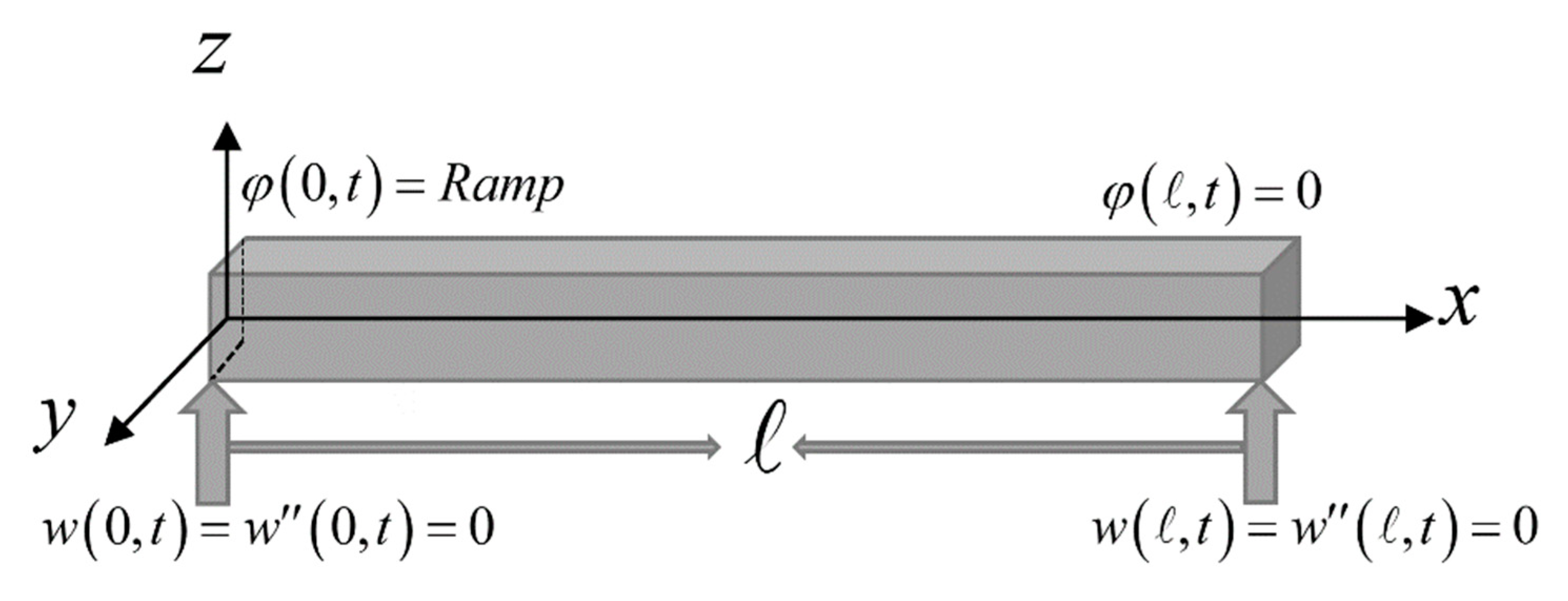
We assume a thin thermoelastic nanobeam with small flexural deflections and the length $\ell$ where $\left(0\le x\le \ell \right)$, width $b$ where $\left(-b/2\le y\le b/2\right)$, and thickness $h$ where $\left(-h/2\le z\le h/2\right)$.

We will assume that the end of the nanobeam $x=0$ is loaded by a known thermal function, and it is simply supported, while the second end of the nanobeam $x=\ell$ is simply supported with zero temperature increment.

The longitudinal, width, and thickness directions of the beam are defined along x, y, and z-axes, respectively; see Figure 1 [22]. For an undeformed and equilibrium case, the nanobeam is unstressed, without any mechanical damping, and the absolute temperature is $T_0$ at any point [6].

The well-known Euler–Bernoulli equation is used in this study. Thus, while bending, any plane cross-section perpendicular to the beam’s axis stays perpendicular to the neutral surface and plane [21,23].

Thus, the components of the displacement are in the form

$$U\left(x,z,t\right)=\left(-z\frac{\partial w\left(x,t\right)}{\partial x},0,w\left(x,t\right)\right)$$

(7)

The cross-section elastic moment is [21,22,24]:

$$M=I\left(\lambda +2\mu \right)\left(1+{\tau }^{\beta }{D}_t^{\beta }\right)\frac{{\partial }^{2}w}{\partial x^2}+\gamma \left(1+{\tau }^{\beta }{D}_t^{\beta }\right)M_T$$

(8)

The equation of motion takes the forms [21,23,24,25]:

$$\frac{{\partial }^{2}M}{\partial x^2}+\rho A\frac{{\partial }^{2}w}{\partial t^2}=0$$

(9)

Moreover, $M_T$ defines the thermal moment of the nanobeam around the x-axis and is given by [21,22,23,24,26]:

$$M_T\left(x,t\right)=b{\displaystyle \underset{-h/2}{\overset{h/2}{\int }}zT\left(x,z,t\right)dz}$$

(10)

where $I=\frac{b{h}^3}{12}$ is defined as the cross-section moment of inertia around the x-axis.

Thus, the lateral deflection governing equation may be written in the following form [19,20,21,23,24,25,26,27]:

$$I\left(\lambda +2\mu \right)\left(1+{\tau }^{\beta }{D}_t^{\beta }\right)\frac{{\partial }^{4}w}{\partial x^4}+\rho A\frac{{\partial }^{2}w}{\partial t^2}+\gamma \left(1+{\tau }^{\beta }{D}_t^{\beta }\right)\frac{{\partial }^2{M}_T}{\partial x^2}=0$$

(11)

where $w=w\left(x,t\right)$ defines the lateral deflection and $A=hb$ denotes the cross-sectional area.

The heat-conduction equations based on the two-temperature model in Equations (3) and (4) take the forms [20,26,27]:

$$\frac{{\partial }^2\phi }{\partial x^2}+\frac{{\partial }^2\phi }{\partial z^2}=\frac{\rho C_{\upsilon }}{K}\left(\frac{\partial }{\partial t}+{\tau }_0\frac{{\partial }^2}{\partial t^2}\right)\theta +\frac{\gamma T_0}{K}\left(1+{\tau }^{\beta }{D}_t^{\beta }\right)\left(\frac{\partial }{\partial t}+{\tau }_0\frac{{\partial }^2}{\partial t^2}\right)e,$$

(12)

and

$$\theta =\phi -a\left(\frac{{\partial }^2\phi }{\partial x^2}+\frac{{\partial }^2\phi }{\partial z^2}\right)$$

(13)

The stress equation takes the form

$${\sigma }_{xx}=\left(1+{\tau }^{\beta }{D}_t^{\beta }\right)\left(\lambda +2\mu \right)e-\gamma \left(1+{\tau }^{\beta }{D}_t^{\beta }\right)\theta$$

(14)

where

$$e=\frac{\partial u}{\partial x}+\frac{\partial v}{\partial y}+\frac{\partial w}{\partial z}$$

(15)

which gives, from (7), that:

$$e=-z\frac{{\partial }^{2}w}{\partial x^2}$$

(16)

Because the beam has no heat transfer through its top and bottom surfaces, we have

$$\frac{\partial }{\partial z}\theta \left(x,\frac{\pm h}{2},t\right)=\frac{\partial }{\partial z}\phi \left(x,\frac{\pm h}{2},t\right)=0$$

(17)

For a thin nanobeam, we consider the temperature changes based on a “$\sin \left(pz\right)$” function along the thickness direction, then [20]:

$$\theta \left(x,z,t\right)={\vartheta }_1\left(x,t\right)\sin \left(pz\right)$$

(18)

and

$$\phi \left(x,z,t\right)={\vartheta }_2\left(x,t\right)\sin \left(pz\right)$$

(19)

where $p=\pi /h$.

Thus, from Equations (10), (11), and (18), we obtain:

$$\begin{array}{l}\left(\lambda +2\mu \right)\left(1+{\tau }^{\beta }{D}_t^{\beta }\right)\frac{{\partial }^{4}w\left(x,t\right)}{\partial x^4}+\frac{12\rho }{h^2}\frac{{\partial }^{2}w\left(x,t\right)}{\partial t^2}+\\ \frac{12\gamma }{h^3}\left(1+{\tau }^{\beta }{D}_t^{\beta }\right)\frac{{\partial }^2{\vartheta }_1\left(x,t\right)}{\partial x^2}{\displaystyle \underset{-h/2}{\overset{h/2}{\int }}z\sin \left(pz\right)dz}=0\end{array}$$

(20)

From Equations (12), (13), (18), and (19), we obtain:

$$\begin{array}{l}\left(\frac{{\partial }^2{\vartheta }_2}{\partial x^2}-p^2{\vartheta }_2\right)\sin \left(pz\right)=\frac{\rho C_{\upsilon }}{K}\left(\frac{\partial }{\partial t}+{\tau }_0\frac{{\partial }^2}{\partial t^2}\right){\vartheta }_1\sin \left(pz\right)-\\ \frac{\gamma T_0}{K}\left(1+{\tau }^{\beta }{D}_t^{\beta }\right)\left(\frac{\partial }{\partial t}+{\tau }_0\frac{{\partial }^2}{\partial t^2}\right)z\frac{{\partial }^{2}w}{\partial x^2}\end{array}$$

(21)

and

$${\vartheta }_1=\left(1+a{p}^2\right){\vartheta }_2-a\frac{{\partial }^2{\vartheta }_2}{\partial x^2}$$

(22)

Hence, Equation (20) gives:

$$\left(\lambda +2\mu \right)\left(1+{\tau }^{\beta }{D}_t^{\beta }\right)\frac{{\partial }^{4}w}{\partial x^4}+\frac{12\rho }{h^2}\frac{{\partial }^{2}w}{\partial t^2}+\frac{12\gamma }{h^3}\left(1+{\tau }^{\beta }{D}_t^{\beta }\right)\frac{{\partial }^2{\vartheta }_1}{\partial x^2}{\displaystyle \underset{-h/2}{\overset{h/2}{\int }}z\sin \left(pz\right)dz}=0$$

(23)

By executing the integrations in the equation above, Equation (23) takes the form:

$$\left(\lambda +2\mu \right)\left(1+{\tau }^{\beta }{D}_t^{\beta }\right)\frac{{\partial }^{4}w}{\partial x^4}+\frac{12\rho }{h^2}\frac{{\partial }^{2}w}{\partial t^2}+\frac{24\gamma }{h{\pi }^2}\left(1+{\tau }^{\beta }{D}_t^{\beta }\right)\frac{{\partial }^2{\vartheta }_1}{\partial x^2}=0$$

(24)

In Equation (21), we multiply z by both sides and complete the integration for z with the boundaries $\left(-h/2\right)\mathrm{and}\left(h/2\right)$; hence, we obtain:

$$\frac{{\partial }^2{\vartheta }_2}{\partial x^2}-p^2{\vartheta }_2=\frac{\rho C_{\upsilon }}{K}\left(\frac{\partial }{\partial t}+{\tau }_0\frac{{\partial }^2}{\partial t^2}\right){\vartheta }_1-\frac{\gamma T_{0}h{\pi }^2}{24K}\left(1+{\tau }^{\beta }{D}_t^{\beta }\right)\left(\frac{\partial }{\partial t}+{\tau }_0\frac{{\partial }^2}{\partial t^2}\right)\frac{{\partial }^{2}w}{\partial x^2}$$

(25)

For simplicity, dimensionless variables will be used as follows [19]:

$$\begin{array}{l}\left({\ell }^{\prime },h^{\prime },x^{\prime },w^{\prime }\right)=\epsilon c_0\left(\ell ,h,x,w\right),\left({{\tau }^{\prime }}_0,t^{\prime },\right)=\epsilon c_0^2\left({\tau }_0,t\right),{\sigma }^{\prime }=\frac{\sigma }{\lambda +2\mu },{\vartheta }_1^{\prime }=\frac{{\vartheta }_1}{T_0},\\ {\vartheta }_2^{\prime }=\frac{{\vartheta }_2}{T_0},a^{\prime }={\epsilon }^2{c}_0^{2}a,\epsilon =\frac{\rho c_0^2}{K},c_0^2=\frac{\lambda +2\mu }{\rho },{\tau }^{\prime }={\left(\epsilon c_0^2\right)}^{\beta }\tau \end{array}$$

(26)

Then, we have

$$\left(1+{\tau }^{\beta }{D}_t^{\beta }\right)\frac{{\partial }^{4}w}{\partial x^4}+{\epsilon }_1\frac{{\partial }^{2}w}{\partial t^2}+{\epsilon }_2\left(1+{\tau }^{\beta }{D}_t^{\beta }\right)\frac{{\partial }^2{\vartheta }_1}{\partial x^2}=0$$

(27)

$$\frac{{\partial }^2{\vartheta }_2}{\partial x^2}-{\epsilon }_3{\vartheta }_2=\left(\frac{\partial }{\partial t}+{\tau }_0\frac{{\partial }^2}{\partial t^2}\right){\vartheta }_1-{\epsilon }_4\left(1+{\tau }^{\beta }{D}_t^{\beta }\right)\left(\frac{\partial }{\partial t}+{\tau }_0\frac{{\partial }^2}{\partial t^2}\right)\frac{{\partial }^{2}w}{\partial x^2}$$

(28)

and

$${\sigma }_{xx}=\left(1+{\tau }^{\beta }{D}_t^{\beta }\right)e-{\epsilon }_5\theta$$

(29)

where ${\epsilon }_1=\frac{12}{h^2},{\epsilon }_2=\frac{24\gamma T_0}{h{\pi }^2\left(\lambda +2\mu \right)},{\epsilon }_3=p^2,{\epsilon }_4=\frac{\gamma h{\pi }^2}{24K\epsilon },{\epsilon }_5\frac{\gamma T_0}{\left(\lambda +2\mu \right)}$.

(We have dropped the prime for convenience.)

4. Problem Formulation in the Laplace Transform Domain

For Equations (27)–(29), the Laplace transform is applied, which is defined as follows:

$$\overline{f}\left(x,s\right)={\displaystyle \underset{0}{\overset{\infty }{\int }}{e}^{-st}f\left(x,t\right)dt}$$

(30)

where the inversion of the Laplace transform may be calculated numerically by the following iteration:

$$f(x,t)=L^{-1}\left[\overline{f}\left(x,s\right)\right]\approx \frac{e^{\kappa t}}{2t}\overline{f}\left(x,\kappa \right)+\frac{e^{\kappa t}}{t}\mathrm{Re}{\displaystyle \sum _{n=1}^N{\left(-1\right)}^n\overline{f}\left(x,\frac{\kappa t+in\pi }{t}\right)}$$

(31)

where “Re” denotes the real part, while “i” defines the imaginary unit number. Numerous numerical tests have been conducted to determine if the value of “$\kappa$” may satisfy the relation $\kappa t\approx 4.7$ [28].

Applying the Laplace transform on the Riemann–Liouville fractional derivative is given by [29]:

$$L\left\{D_t^{\beta }f\left(t\right)\right\}=\left\{\begin{array}{cc}{s}^{\beta }\overline{f}\left(s\right)& 0\le \beta <1\\ s\overline{f}\left(s\right)& \beta =1\end{array}\right\},$$

(32)

where the initial conditions which have been used are given by:

$${\vartheta }_1\left(x,0\right)={\vartheta }_2\left(x,0\right)=w\left(x,0\right)={\frac{\partial {\vartheta }_1\left(x,t\right)}{\partial t}|}_{t=0}={\frac{\partial {\vartheta }_2\left(x,t\right)}{\partial t}|}_{t=0}={\frac{\partial w\left(x,t\right)}{\partial t}|}_{t=0}=0$$

(33)

Hence, the following system of ordinary differential equations has been obtained:

$$\frac{d^4\overline{w}}{d{x}^4}+{\epsilon }_6\overline{w}+{\epsilon }_2\frac{d^2{\overline{\vartheta }}_1}{d{x}^2}=0$$

(34)

$$\frac{d^2{\overline{\vartheta }}_2}{d{x}^2}-{\epsilon }_3{\overline{\vartheta }}_2={\epsilon }_7{\overline{\vartheta }}_1-{\epsilon }_8\frac{d^2\overline{w}}{d{x}^2}$$

(35)

$${\overline{\vartheta }}_1=\left(1+a{p}^2\right){\overline{\vartheta }}_2-a\frac{d^2{\overline{\vartheta }}_2}{d{x}^2}$$

(36)

and

$${\overline{\sigma }}_{xx}=\left(1+\tau s^{\beta }\right)\overline{e}-{\epsilon }_5\left(1+\tau s^{\beta }\right)\overline{\theta }$$

(37)

Moreover, we have

$$\overline{e}=-z\frac{d^2\overline{w}}{d{x}^2}$$

(38)

where ${\epsilon }_6=\frac{{\epsilon }_1{s}^2}{\left(1+\tau s^{\beta }\right)}$, ${\epsilon }_7=\left(s+{\tau }_0{s}^2\right),{\epsilon }_8={\epsilon }_4\left(1+\tau s^{\beta }\right)\left(s+{\tau }_0{s}^2\right)$.

Hence, we have:

$$\frac{d^4\overline{w}}{d{x}^4}+{\epsilon }_6\overline{w}+{\alpha }_1\frac{d^2{\overline{\vartheta }}_2}{d{x}^2}-a{\epsilon }_2\frac{d^4{\overline{\vartheta }}_2}{d{x}^4}=0$$

(39)

$${\alpha }_2\frac{d^2\overline{w}}{d{x}^2}+\frac{d^2{\overline{\vartheta }}_2}{d{x}^2}-{\alpha }_3{\overline{\vartheta }}_2=0$$

(40)

where ${\alpha }_1={\epsilon }_2\left(1+a{p}^2\right)$, ${\alpha }_2=\frac{{\epsilon }_8}{\left(1+a{\epsilon }_7\right)}$, ${\alpha }_3=\frac{{\epsilon }_3+{\epsilon }_7\left(1+a{p}^2\right)}{\left(1+a{\epsilon }_7\right)}$.

The above system of equations gives the following characteristic equations:

$$\left(\frac{d^6}{d{x}^6}-L\frac{d^4}{d{x}^4}+M\frac{d^2}{d{x}^2}-N\right)\left\{{\overline{\vartheta }}_2,\overline{w}\right\}=0$$

(41)

where $L={\alpha }_3-a{\alpha }_2{\epsilon }_2,M={\epsilon }_6-{\alpha }_1{\alpha }_2,N={\alpha }_3{\epsilon }_6$.

The general solutions of Equation (41)—where the second end of nanobeam $x=\ell$ is simply supported with zero temperature increment—will take the forms:

$${\overline{\vartheta }}_2\left(x,s\right)={\displaystyle \sum _{i=1}^3{A}_i\sinh \left(k_i\left(\ell -x\right)\right)}$$

(42)

and

$$\overline{w}\left(x,s\right)={\displaystyle \sum _{i=1}^3{A}_i{w}_i\sinh \left(k_i\left(\ell -x\right)\right)}$$

(43)

where $A_i\mathrm{and}{w}_i$ are some parameters to be determined and $\pm k_1,\pm k_2\mathrm{and}\pm k_3$ denote the solutions of the following characteristic equation:

$$k^6-L{k}^4+M{k}^2-N=0$$

(44)

To obtain $w_i$, we will substitute from Equations (42) and (43) into Equation (40); hence, we have

$$w_i=\frac{{\alpha }_3-k_i^2}{{\alpha }_2{k}_i^2}$$

(45)

Then, we obtain

$$\overline{w}\left(x,s\right)={\displaystyle \sum _{i=1}^3\frac{{\alpha }_3-k_i^2}{{\alpha }_2{k}_i^2}{A}_i\sinh \left(k_i\left(\ell -x\right)\right)}$$

(46)

To obtain $A_1,A_2,\mathrm{and}{A}_3$, certain boundary conditions are used; thus, we assume the end of the nanobeam $x=0$ is loaded by the thermal function $g\left(t\right)$ and is simply supported.

Hence, we have:

$$w\left(0,t\right)=\frac{{\partial }^{2}w\left(0,t\right)}{\partial x^2}=0,{\vartheta }_2\left(0,t\right)={\vartheta }_{0}g\left(t\right)$$

(47)

where ${\vartheta }_0$ is constant.

Applying the Laplace transform gives:

$$\overline{w}\left(0,s\right)=\frac{{\partial }^2\overline{w}\left(0,s\right)}{\partial x^2}=0$$

(48)

and

$${\overline{\vartheta }}_2\left(0,s\right)={\vartheta }_0\overline{g}\left(s\right)$$

(49)

Hence, the following system of linear equations was obtained:

$${\displaystyle \sum _{i=1}^3{A}_i\sinh \left(k_i\ell \right)}={\vartheta }_0\overline{g}\left(s\right)$$

(50)

$${\displaystyle \sum _{i=1}^3\frac{{\alpha }_3-k_i^2}{{\alpha }_2{k}_i^2}{A}_i\sinh \left(k_i\ell \right)}=0$$

(51)

and

$${\displaystyle \sum _{i=1}^3\frac{{\alpha }_3-k_i^2}{{\alpha }_2}{A}_i\sinh \left(k_i\ell \right)}=0$$

(52)

After solving the above system, then, we obtain $A_1=\frac{{\vartheta }_0\overline{g}\left(s\right)k_1^2\left(k_2^2-{\alpha }_3\right)\left(k_3^2-{\alpha }_3\right)}{{\alpha }_3\left(k_1^2-k_2^2\right)\left(k_1^2-k_3^2\right)\sinh \left(k_1\ell \right)}$, $A_2=\frac{{\vartheta }_0\overline{g}\left(s\right)k_2^2\left(k_1^2-{\alpha }_3\right)\left(k_3^2-{\alpha }_3\right)}{{\alpha }_3\left(k_2^2-k_1^2\right)\left(k_2^2-k_3^2\right)\sinh \left(k_2\ell \right)}$, $A_3=\frac{{\vartheta }_0\overline{g}\left(s\right)k_3^2\left(k_2^2-{\alpha }_3\right)\left(k_1^2-{\alpha }_3\right)}{{\alpha }_3\left(k_3^2-k_1^2\right)\left(k_3^2-k_2^2\right)\sinh \left(k_3\ell \right)}$.

Then, the solutions in the Laplace transform domain are as follows:

$$\overline{\phi }\left(x,z,s\right)=\frac{{\vartheta }_0\overline{g}\left(s\right)\sin \left(pz\right)}{{\alpha }_3}\left[\begin{array}{l}\frac{\left(k_2^2-{\alpha }_3\right)\left(k_3^2-{\alpha }_3\right)k_1^2}{\left(k_1^2-k_2^2\right)\left(k_1^2-k_3^2\right)\sinh \left(k_1\ell \right)}\sinh \left(k_1\left(\ell -x\right)\right)+\\ \frac{\left(k_1^2-{\alpha }_3\right)\left(k_3^2-{\alpha }_3\right)k_2^2}{\left(k_2^2-k_1^2\right)\left(k_2^2-k_3^2\right)\sinh \left(k_2\ell \right)}\sinh \left(k_2\left(\ell -x\right)\right)+\\ \frac{\left(k_2^2-{\alpha }_3\right)\left(k_1^2-{\alpha }_3\right)k_3^2}{\left(k_3^2-k_1^2\right)\left(k_3^2-k_2^2\right)\sinh \left(k_3\ell \right)}\sinh \left(k_3\left(\ell -x\right)\right)\end{array}\right]$$

(53)

The lateral deflection is:

$$\overline{w}\left(x,s\right)={\vartheta }_0\overline{g}\left(s\right)\left(a{\alpha }_3{\epsilon }_2-{\alpha }_1\right)\left[\begin{array}{l}\frac{\sinh \left(k_1\left(\ell -x\right)\right)}{\left(k_1^2-k_2^2\right)\left(k_1^2-k_3^2\right)\sinh \left(k_1\ell \right)}+\\ \frac{\sinh \left(k_2\left(\ell -x\right)\right)}{\left(k_2^2-k_1^2\right)\left(k_2^2-k_3^2\right)\sinh \left(k_2\ell \right)}+\\ \frac{\sinh \left(k_3\left(\ell -x\right)\right)}{\left(k_3^2-k_1^2\right)\left(k_3^2-k_2^2\right)\sinh \left(k_3\ell \right)}\end{array}\right]$$

(54)

and the strain from Equation (38) takes the form:

$$\overline{e}\left(x,z,s\right)=-z{\vartheta }_0\overline{g}\left(s\right)\left(a{\alpha }_3{\epsilon }_2-{\alpha }_1\right)\left[\begin{array}{l}\frac{k_1^2\sinh \left(k_1\left(\ell -x\right)\right)}{\left(k_1^2-k_2^2\right)\left(k_1^2-k_3^2\right)\sinh \left(k_1\ell \right)}+\\ \frac{k_2^2\sinh \left(k_2\left(\ell -x\right)\right)}{\left(k_2^2-k_1^2\right)\left(k_2^2-k_3^2\right)\sinh \left(k_2\ell \right)}+\\ \frac{k_3^2\sinh \left(k_3\left(\ell -x\right)\right)}{\left(k_3^2-k_1^2\right)\left(k_3^2-k_2^2\right)\sinh \left(k_3\ell \right)}\end{array}\right]$$

(55)

5. The Function of the Strain Energy Density

The strain energy density function, which is generated on the beam, is given by [1,30,31]:

$$\varpi \left(x,z,t\right)=\frac{1}{2}{\displaystyle \sum _{i,j=1}^3{e}_{ij}{\sigma }_{ij}}=\frac{1}{2}e\left(x,z,t\right){\sigma }_{xx}\left(x,z,t\right)$$

(56)

Thus, we obtain

$$\varpi \left(x,z,t\right)=\frac{1}{2}\left[L^{-1}\left(\overline{e}\left(x,z,s\right)\right)\right]\left[L^{-1}\left({\overline{\sigma }}_{xx}\left(x,z,s\right)\right)\right]$$

(57)

where $L^{-1}[•]$ defines the Laplace transform inversion.

The thermal loading has a ramp-type heat as follows:

$$g\left(t\right)=\left\{\begin{array}{cc}\frac{t}{t_0}& 0<t<t_0\\ 1& t\ge t_0\end{array}\right\}$$

(58)

where $t_0$ is the ramp-type heat time parameter.

Hence, we have

$$\overline{g}\left(s\right)=\frac{1-e^{-s{t}_0}}{s^2{t}_0}$$

(59)

6. Numerical Results and Discussion

For computational findings, silicon nitride was used as a thermoelastic material, and the values of the physical constants are given by [19,25,27]:

${\alpha }_T=2.71{\left(10\right)}^{-6}{\mathrm{K}}^{-1}$, $k=43.5\mathrm{W}/\left(\mathrm{m}\mathrm{K}\right)$, $T_0=293\mathrm{K}$, $\rho =3200\mathrm{kg}/{\mathrm{m}}^3$, $C_{\upsilon }=630\mathrm{J}/\left(\mathrm{kg}\mathrm{K}\right)$, ${\lambda }_0=217\times {10}^9\mathrm{N}/{\mathrm{m}}^2$, ${\mu }_0=108\times {10}^9\mathrm{N}/{\mathrm{m}}^2$, ${\tau }_0=4.32\times {10}^{-13}\mathrm{s}$.

The aspect ratios of the nanobeam are fixed as $\ell /h=5$ and $b=h/4$, and the range of the nanobeam length $\ell$ is $\left(1-100\right)\times {10}^{-12}\mathrm{m}$.

The value of the original time t (sec) is of the order of ${10}^{-12}$, while the initial values of the thermal relaxation time ${\tau }_0\left(\sec \right)$ and mechanical relaxation time $\tau \left(\sec \right)$ are of the order of ${10}^{-14}$.

After using the dimensionless variables of the nanobeam, the figures are prepared; thus, we have $\ell =1.0$, ${\theta }_0=1.0$, ${\tau }_0=0.01$, $t=1.0$, and we consider $z=h/4$.

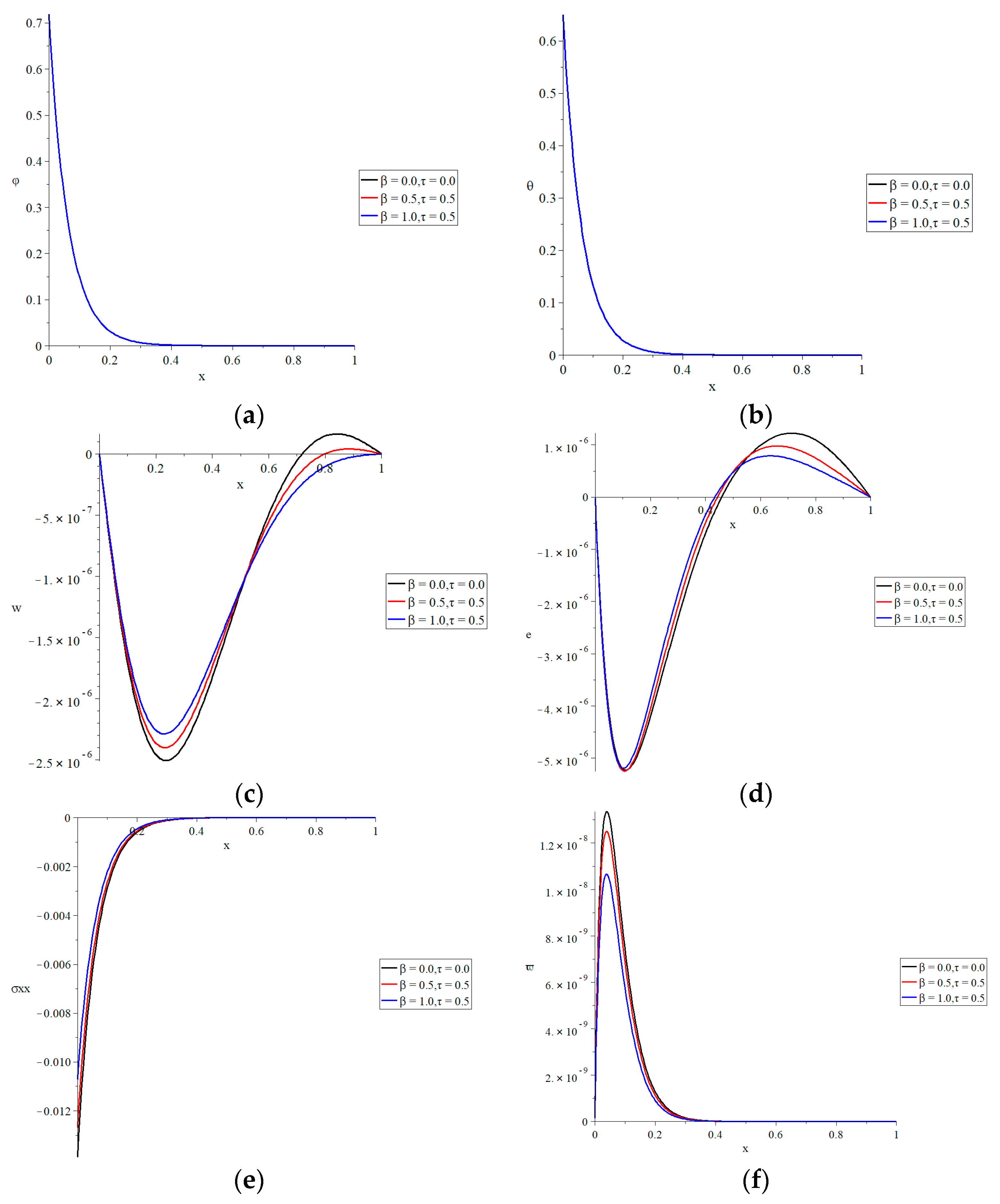
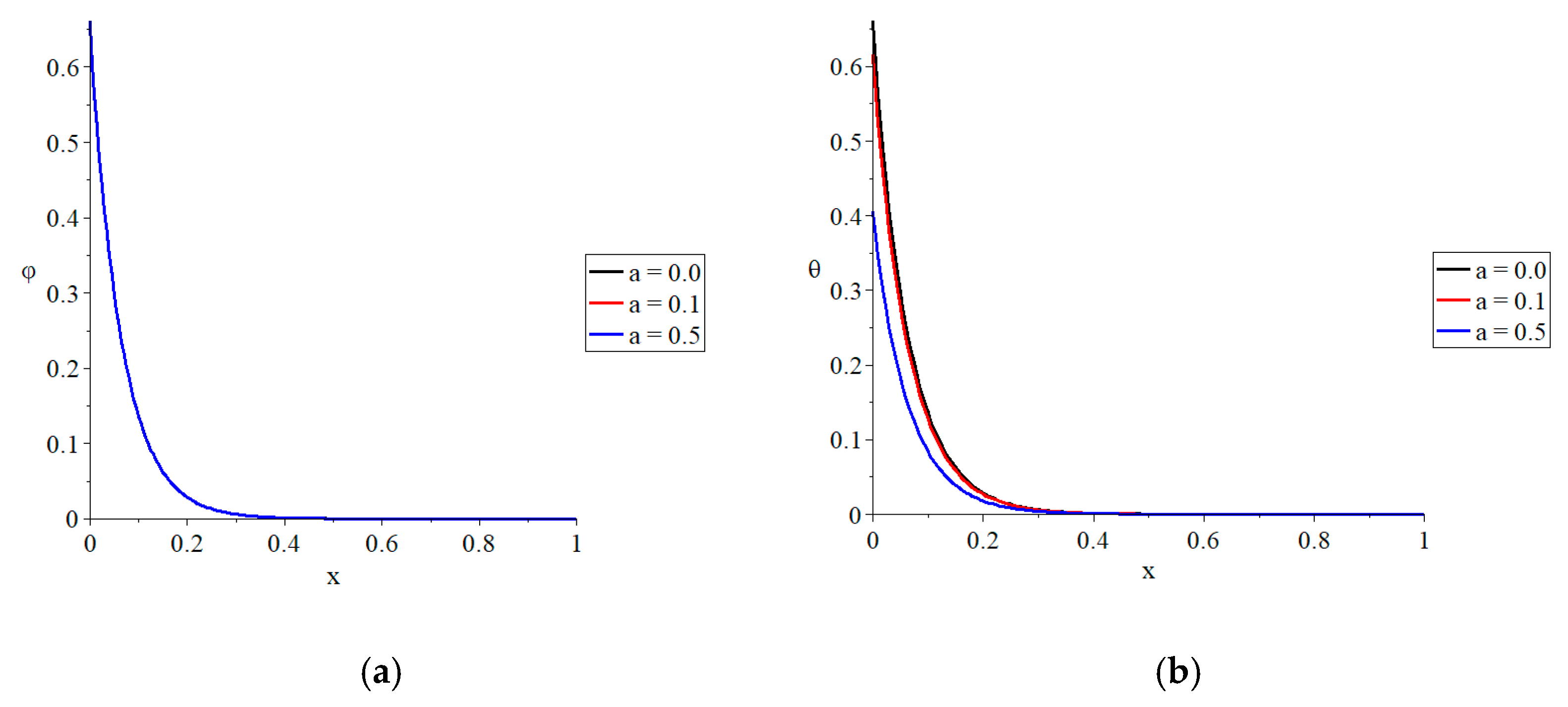
Figure 2 represents the conductive temperature increment, dynamical temperature increment, lateral deflection, strain, stress, and strain energy density function distributions for various values of the parameter of the fractional-order strain $\beta =\left(0.0,0.5,1.0\right)$ when $t_0=1.0$ in the context of the two-temperature model $\left(a=0.1\right)$, respectively. The value $\beta =0.0$ includes $\tau =0.0$, the traditional material in the context of classical strain, while the values $\beta =\left(0.5,1.0\right)$ represent the non-classical strain based on fractional-order theory.

Figure 2a,b shows that the effect of the fractional-order strain parameter $\beta$ causes a minor effect on the thermal waves, such as a dynamical and conductive temperature increment. The initial value of the conductive temperature is higher than the initial value of the dynamical temperature due to the impact of the two-temperature parameter.

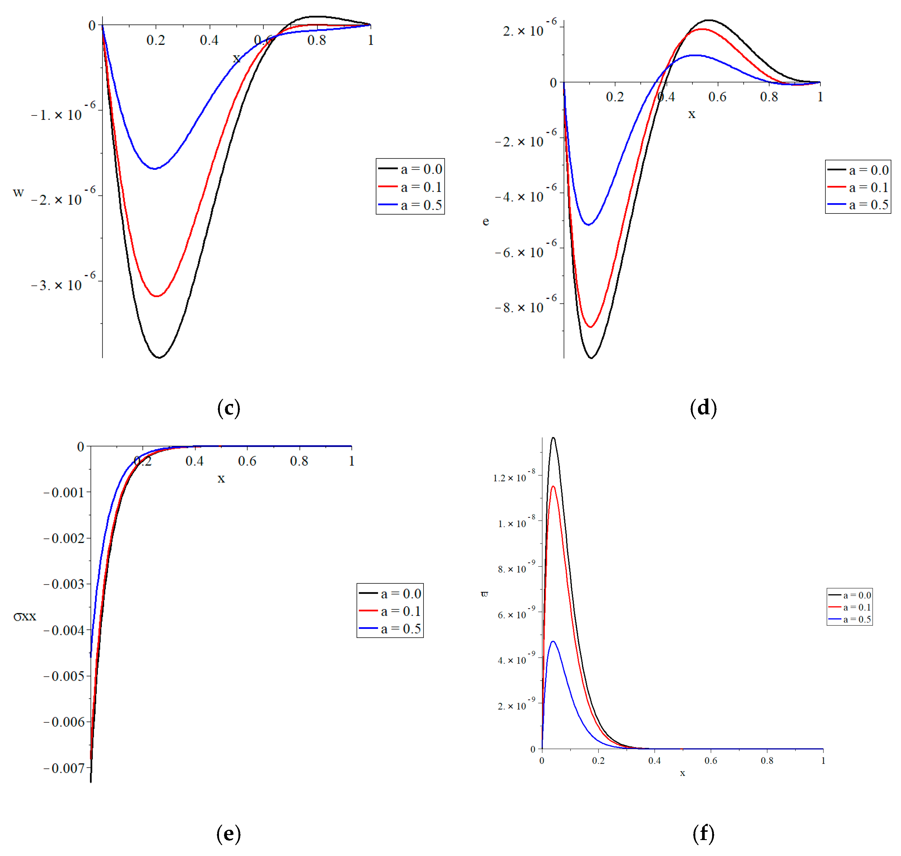
Figure 2c shows that the fractional-order strain parameter has a significant influence on the lateral deflection function. When the fractional-order strain parameter is increased, the absolute value of the lateral deflection function decreases. For the lateral-deflection function, the absolute values of the maximum points are in the following order:

$$\left|w_{\max }\left(\beta =0.0\right)\right|>\left|w_{\max }\left(\beta =0.5\right)\right|>\left|w_{\max }\left(\beta =1.0\right)\right|$$

(60)

Figure 2d shows that the fractional-order strain parameter has a major impact on the strain function. Increases in the fractional-order strain parameter result in a drop in the absolute value of the strain function.

The absolute values of the strain function’s maximum points are in the following order:

$$\left|e_{\max }\left(\beta =0.0\right)\right|>\left|e_{\max }\left(\beta =0.5\right)\right|>\left|e_{\max }\left(\beta =1.0\right)\right|$$

(61)

Figure 2e shows that the fractional-order strain parameter has a major effect on the stress function. An increase in the fractional-order strain parameter causes a decrease in the absolute value of the stress function. The absolute value of the start points of the stress function takes the following order:

$$\left|{\sigma }_{\max }\left(\beta =0.0\right)\right|>\left|{\sigma }_{\max }\left(\beta =0.5\right)\right|>\left|{\sigma }_{\max }\left(\beta =1.0\right)\right|$$

(62)

Figure 2f shows that the fractional-order strain parameter has a substantial influence on the strain energy density function. An increase in the fractional-order strain parameter causes a decrease in the strain energy density function. The values of the maximum points of the strain energy density function are in the order as follows:

$${\varpi }_{\max }\left(\beta =0.0\right)>{\varpi }_{\max }\left(\beta =0.5\right)>{\varpi }_{\max }\left(\beta =1.0\right)$$

(63)

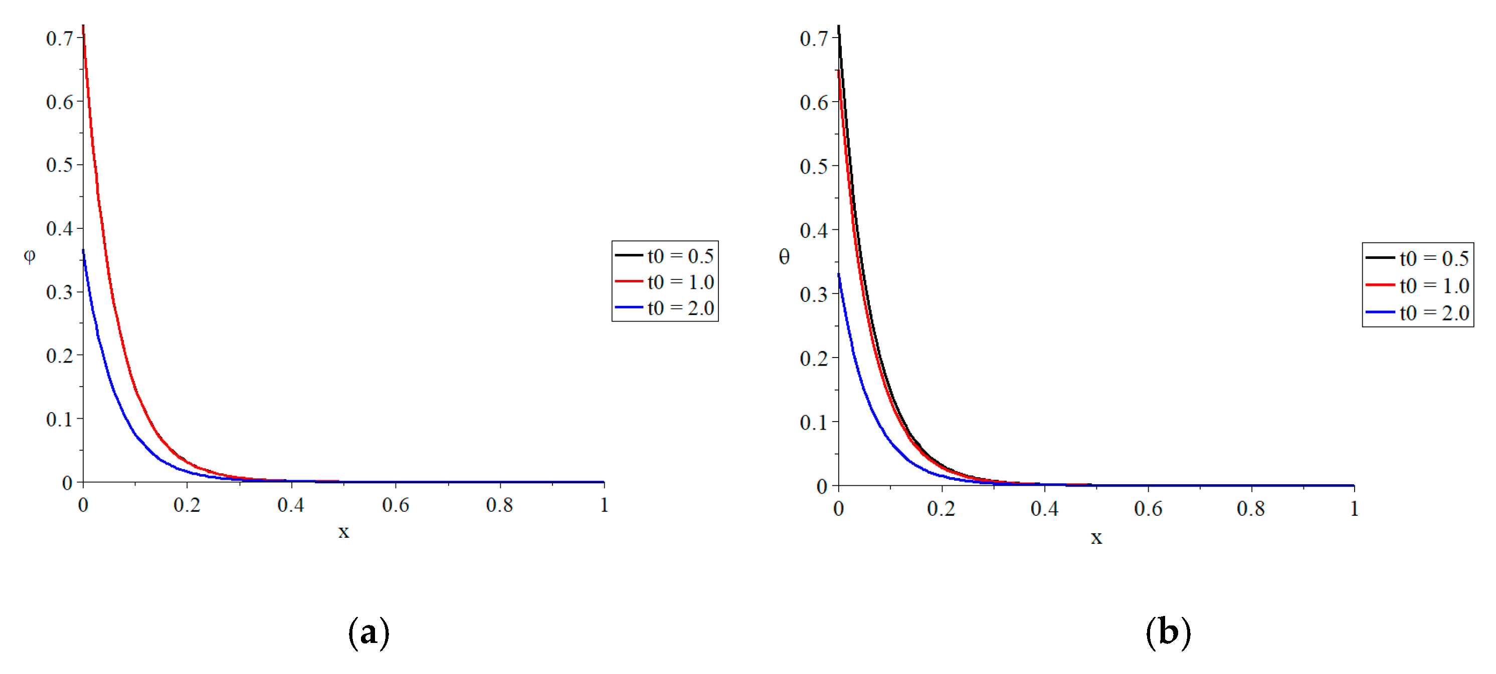
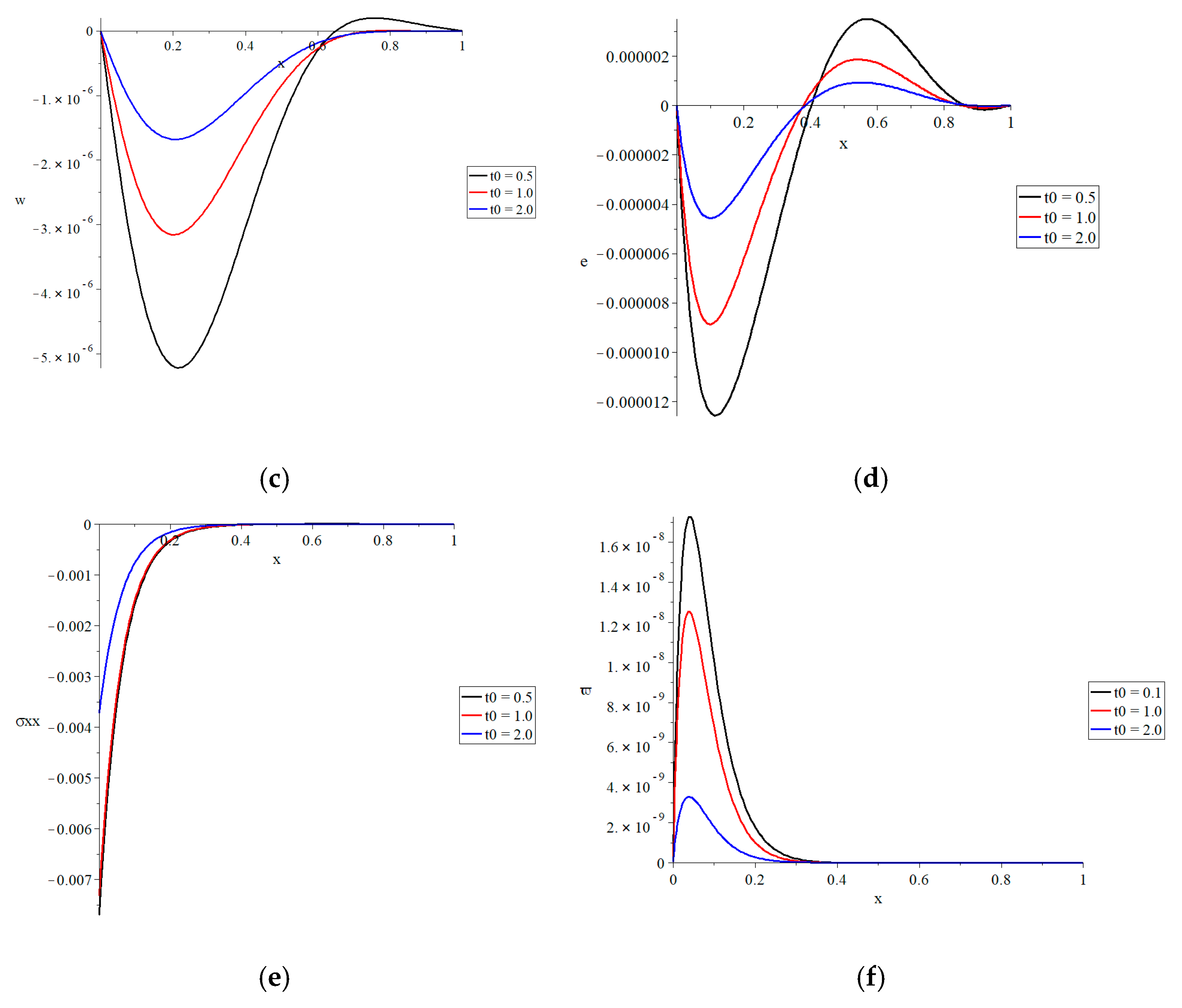
Figure 3 represents the conductive temperature increment; dynamical temperature increment; lateral deflection; and strain, stress, and strain energy density function distributions in the context of the two-temperature model when $a=0.1$ and $\beta =1.0$, for three values of the ramp-type heat parameter $t_0=\left(0.5,1.0,2.0\right)$. The value $t_0=0.5$ represents $t>t_0$, the value $t_0=1.0$ represents $t=t_0$, and the value $t_0=2.0$ represents $t<t_0$. The ramp-type heat parameter has been shown to have a substantial influence on all of the functions investigated. Increases in the ramp-type heat parameter result in decreases in the dynamical temperature increment, conductive temperature increment, lateral deflection, and strain, stress, and strain energy density function.

Figure 4 represents the conductive temperature, dynamical temperature, lateral deflection, and strain, stress, and strain energy density function distributions in the context of the two-temperature model when $t_0=1.0$ and $\beta =1.0$ for various values of the two-temperature parameter $a=\left(0.0,0.1,0.5\right)$. The value $a=0.0$ represents the one-temperature thermoelasticity theory (L–S), while the values $a=\left(0.1,0.5\right)$ represent the two-temperature thermoelasticity theory (Youssef). Except for the conductive-temperature-increase function, the two-temperature parameter has a substantial influence on the dynamical temperature increment, conductive temperature increment, lateral deflection, and strain, stress, and strain energy density function. The internal data in Figure 4 demonstrate that as the two-temperature parameter increases, the conductive temperature increment, lateral deflection, and strain, stress, and strain energy density functions all drop.

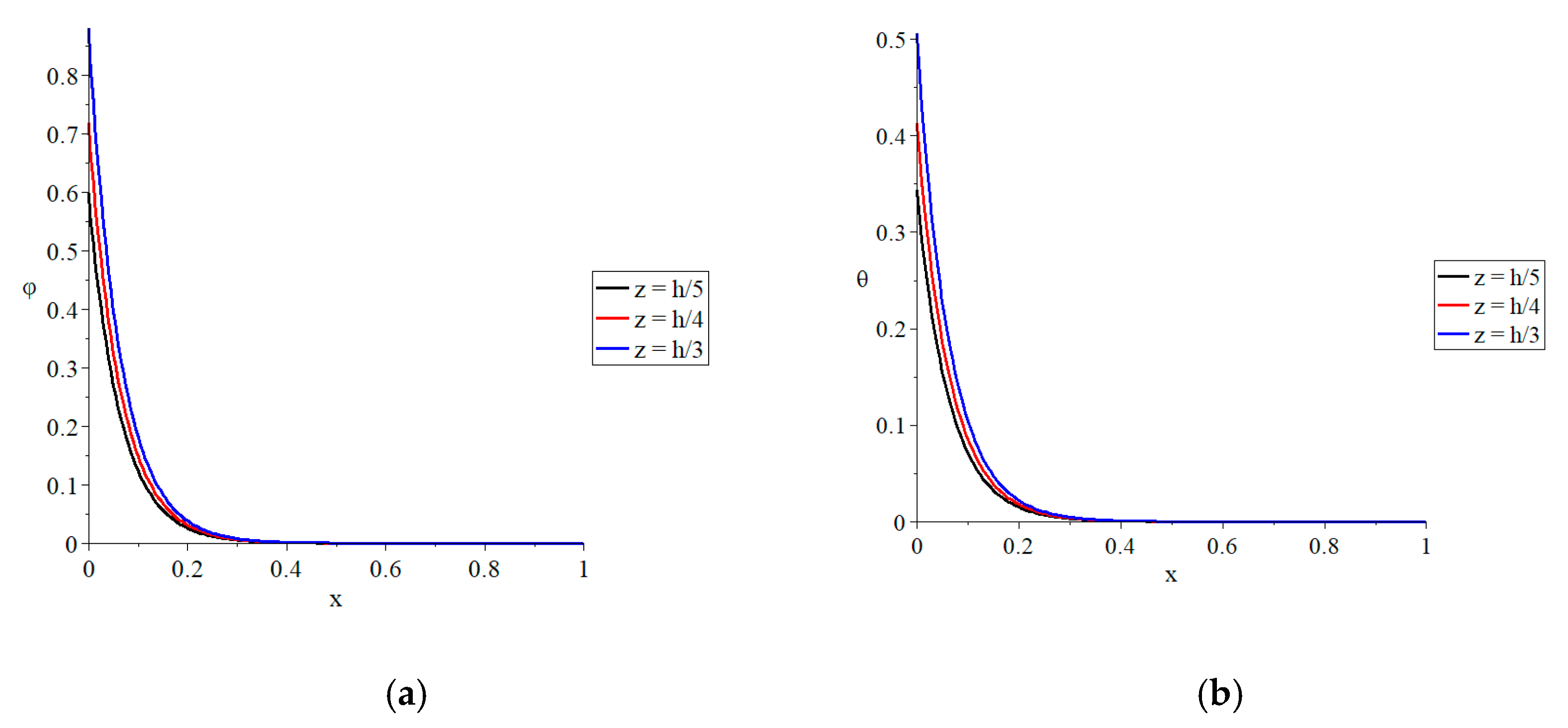
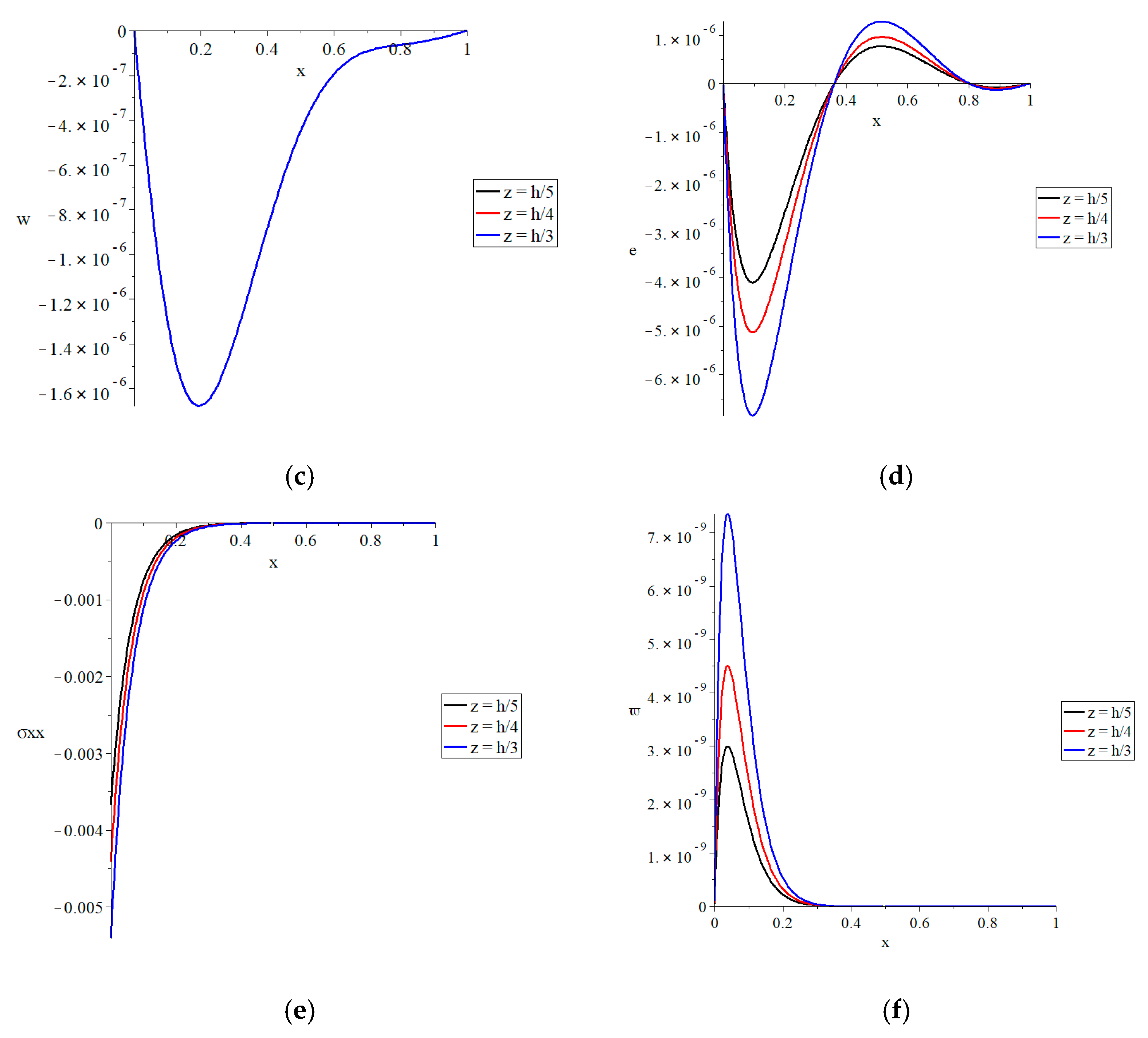
Figure 5 represents the conductive and dynamical temperature, lateral deflection, and strain, stress, and strain energy density function distributions for three different values of the beam’s thickness $z=\left(h/5,h/4,h/3\right)$ when $\beta =1.0,t_0=1.0,\mathrm{and}a=0.5$, respectively. The thickness of the beam has a substantial effect on the conductive and dynamical temperatures, as well as the strain, stress, and strain energy density function distributions, but it has no impact on the lateral deflection, which is unaffected by the variable z. The values of the conductive and dynamical temperatures, absolute values of the strain, absolute values of the stress, and strain energy density function all rise as the thickness of the beam increases.

To validate the current results, we can compare the current results with the results of Youssef and El-Bary [21]. We can see that the distributions of the studied functions in Figures 2–8 in [21] have the same behaviors as the figures in the current work.

7. Conclusions

Under fractional-order strain and two-temperature considerations, a simply supported, thermoelastic, isotropic, and homogeneous nanobeam has been thermally loaded using ramp heating.

The fractional-order strain parameter, two-temperature parameter, ramp-type heat parameter, and thickness of the nanobeam all have a substantial influence on the thermal and mechanical waves; however, the effects of the fractional-order strain parameter are only very limited for the thermal waves.

The ramp-type heat parameter may be utilized to control the thermomechanical waves’ propagation and the energy passing through the nanobeam resonator.

According to the current results and the results in similar papers, we can declare that the fractional-order strain has no major effects on heat conduction or thermal waves in general.

References

1. Biot, M.A. Thermoelasticity and irreversible thermodynamics. J. Appl. Phys. 1956, 27, 240–253. [Google Scholar] [CrossRef]
2. Lord, H.W.; Shulman, Y. A generalized dynamical theory of thermoelasticity. J. Mech. Phys. Solids 1967, 15, 299–309. [Google Scholar] [CrossRef]
3. Dhaliwal, R.S.; Sherief, H.H. Generalized thermoelasticity for anisotropic media. Q. Appl. Math. 1980, 38, 1–8. [Google Scholar] [CrossRef] [Green Version]
4. Hoang, C.M. Thermoelastic damping depending on vibration modes of nano beam resonator. Commun. Phys. 2015, 25, 317. [Google Scholar] [CrossRef] [Green Version]
5. Naik, A.K.; Hanay, M.; Hiebert, W.; Feng, X.; Roukes, M.L. Towards single-molecule nanomechanical mass spectrometry. Nat. Nanotechnol. 2009, 4, 445. [Google Scholar] [CrossRef] [PubMed]
6. O’Connell, A.D.; Hofheinz, M.; Ansmann, M.; Bialczak, R.C.; Lenander, M.; Lucero, E.; Neeley, M.; Sank, D.; Wang, H.; Weides, M. Quantum ground state and single-phonon control of a mechanical resonator. Nature 2010, 464, 697. [Google Scholar] [CrossRef]
7. van Beek, J.; Puers, R. A review of MEMS oscillators for frequency reference and timing applications. J. Micromech. Microeng. 2011, 22, 013001. [Google Scholar] [CrossRef]
8. Sharma, J.; Grover, D. Thermoelastic vibrations in micro-/nano-scale beam resonators with voids. J. Sound Vib. 2011, 330, 2964–2977. [Google Scholar] [CrossRef]
9. Sun, Y.; Saka, M. Thermoelastic damping in micro-scale circular plate resonators. J. Sound Vib. 2010, 329, 328–337. [Google Scholar] [CrossRef]
10. Lifshitz, R.; Roukes, M.L. Thermoelastic damping in micro-and nanomechanical systems. Phys. Rev. B 2000, 61, 5600. [Google Scholar] [CrossRef] [Green Version]
11. Al-Huniti, N.S.; Al-Nimr, M.; Naji, M. Dynamic response of a rod due to a moving heat source under the hyperbolic heat conduction model. J. Sound Vib. 2001, 242, 629–640. [Google Scholar] [CrossRef]
12. Al-Lehaibi, E.A.; Youssef, H.M. Vibration of gold nano-beam with variable young’s modulus due to thermal shock. World J. Nano Sci. Eng. 2015, 5, 194. [Google Scholar] [CrossRef] [Green Version]
13. Boley, B.A. Approximate analyses of thermally induced vibrations of beams and plates. J. Appl. Mech. 1972, 39, 212–216. [Google Scholar] [CrossRef]
14. Kidawa-Kukla, J. Application of the Green functions to the problem of the thermally induced vibration of a beam. J. Sound Vib. 2003, 262, 865–876. [Google Scholar] [CrossRef]
15. Manolis, G.; Beskos, D. Thermally induced vibrations of beam structures. Comput. Methods Appl. Mech. Eng. 1980, 21, 337–355. [Google Scholar] [CrossRef]
16. Youssef, H.M. Theory of two-temperature-generalized thermoelasticity. IMA J. Appl. Math. 2006, 71, 383–390. [Google Scholar] [CrossRef]
17. Magin, R.L.; Royston, T.J. Fractional-order elastic models of cartilage: A multi-scale approach. Commun. Nonlinear Sci. Numer. Simul. 2010, 15, 657–664. [Google Scholar] [CrossRef]
18. Youssef, H.M. Theory of generalized thermoelasticity with fractional order strain. J. Vib. Control. 2016, 22, 3840–3857. [Google Scholar] [CrossRef]
19. Grover, D. Transverse vibrations in micro-scale viscothermoelastic beam resonators. Arch. Appl. Mech. 2013, 83, 303–314. [Google Scholar] [CrossRef]
20. Youssef, H.M.; El-Bary, A.A. Two-Temperature Thermoelastic Damping of a Gold Nano-Beam Resonator with Variable Young’s Modulus. Int. J. Acoust. Vib. 2019, 24, 540–545. [Google Scholar] [CrossRef]
21. Youssef, H.M.; El-Bary, A.A. Generalized fractional viscothermoelastic nanobeam under the classical Caputo and the new Caputo–Fabrizio definitions of fractional derivatives. Waves Random Complex Media 2021, 1–22. [Google Scholar] [CrossRef]
22. Youssef, H.M.; El-Bary, A.A. Characterization of the thermal quality factor of two-temperature micro-viscothermoelastic resonator due to static-pre-stress based on dual-phase-lagging heat conduction. Alex. Eng. J. 2020, 59, 3919–3926. [Google Scholar] [CrossRef]
23. Grover, D.; Seth, R. Generalized viscothermoelasticity theory of dual-phase-lagging model for damping analysis in circular micro-plate resonators. Mech. Time Depend. Mater. 2019, 23, 119–132. [Google Scholar] [CrossRef]
24. Grover, D.; Seth, R. Viscothermoelastic micro-scale beam resonators based on dual-phase lagging model. Microsyst. Technol. 2018, 24, 1667–1672. [Google Scholar] [CrossRef]
25. Grover, D. Damping in thin circular viscothermoelastic plate resonators. Can. J. Phys. 2015, 93, 1597–1605. [Google Scholar] [CrossRef]
26. Youssef, H.M.; Al-Hazmi, M.W. The influence of the static-pre-stress and mechanical damage variable in the thermal quality factor of two-temperature viscothermoelastic resonators. Adv. Mech. Eng. 2020, 12, 1–9. [Google Scholar] [CrossRef]
27. Grover, D. Viscothermoelastic vibrations in micro-scale beam resonators with linearly varying thickness. Can. J. Phys. 2012, 90, 487–496. [Google Scholar] [CrossRef]
28. Tzou, D. Macro- to Microscale Heat Transfer, The Lagging Behavior; Taylor Francis: Washington, DC, USA, 1997. [Google Scholar]
29. Podlubny, I. Fractional Differential Equations: An Introduction to Fractional Derivatives, Fractional Differential Equations, to Methods of Their Solution and Some of Their Applications; Academic Press: Cambridge, MA, USA, 1998. [Google Scholar]
30. Biot, M.A. Theory of stress-strain relations in anisotropic viscoelasticity and relaxation phenomena. J. Appl. Phys. 1954, 25, 1385–1391. [Google Scholar] [CrossRef]
31. Biot, M.A. Variational principles in irreversible thermodynamics with application to viscoelasticity. Phys. Rev. 1955, 97, 1463. [Google Scholar] [CrossRef] [Green Version]
Figure 1. Rectangular thermoelastic nanobeam.
Mca 26 00078 g001
Figure 2. The distributions with variance fractional-order strain parameter when t 0 = 1.0 ,   a = 0.1 . (a) The distribution of conductive temperature, (b) the distribution of dynamic temperature, (c) the distribution of lateral deflection, (d) the distribution of strain, (e) the distribution of deformation stress, and (f) the distribution of strain energy density function.
Mca 26 00078 g002
Figure 3. The distributions with variance ramp-type heat parameter when β = 1.0 ,   a = 0.1 . (a) The distribution of conductive temperature, (b) the distribution of dynamical temperature, (c) the distribution of lateral deflection, (d) the distribution of strain, (e) the distribution of stress, (f) the distribution of strain energy density function.
Mca 26 00078 g003aMca 26 00078 g003b
Figure 4. The distributions with variance values of the two-temperature parameter when β = 1.0 ,   t 0 = 1.0 . (a) The distribution of conductive temperature, (b) the distribution of dynamical temperature, (c) the distribution of lateral deflection, (d) distribution of strain, (e) the distribution of stress, (f) the distribution of strain energy density function.
Mca 26 00078 g004aMca 26 00078 g004b
Figure 5. The distributions with variance thickness z when β = 1.0 ,   t 0 = 1.0 ,   a = 0.5 . (a) The distribution of conductive temperature, (b) the distribution of dynamical temperature, (c) the distribution of lateral deflection, (d) the distribution of strain, (e) the distribution of stress, (f) the distribution of strain energy density function.
Mca 26 00078 g005aMca 26 00078 g005b
Publisher’s Note: MDPI stays neutral with regard to jurisdictional claims in published maps and institutional affiliations.