Alternative Initial Probability Tables for Elicitation of Bayesian Belief Networks

Abstract

Bayesian Belief Networks are used in many fields of application. Defining the conditional dependencies via conditional probability tables requires the elicitation of expert belief to fill these tables, which grow very large quickly. In this work, we propose two methods to prepare these tables based on a low number of input parameters using specific structures and one method to generate the table using probability tables of each relation of a child node with a certain parent. These tables can be used further as a starting point for elicitation.

1. Introduction

A Bayesian Belief Network (BBN) is a probabilistic graphical model that represents a set of variables and their conditional dependencies via a directed acyclic graph. Bayesian networks can be used for probabilistic reasoning, deriving the effects of the occurrence of an event by predicting the likelihood of other related events. The use of BBNs has seen an enormous increase in recent years. Examples can be found in all kinds of application areas where complex systems are found, such as natural ecosystems [1,2], human behavior [3,4], risk assessment in constructions and complex technological systems [5,6,7,8], military operations [9,10,11], medicine and healthcare [12,13] and business and cyber threat analysis [14,15].

The main idea of a BBN is that it specifies the relations between variables, capturing the probability that a variable has a specific state, depending on the state of other variables, its parents. If we have three variables, X, Y and Z, each having two possible states (0, 1), and the state of X depends on the state of Y and Z, which are mutually independent, the marginal probability of X being 1 can be derived:

$$P(X=1)=\sum _{i,j\in \{0,1\}}P(X=1|Y=i,Z=j)P(Y=i)P(Z=j).$$

(1)

An example is depicted in Figure 1. The figure was created using the BBN tool Genie (www.bayesfusion.com/genie, accessed on 23 July 2021).

Important here is that the conditional probability $P\left(X\right|Y,Z)$ has to be specified. In the example in Figure 1, this means a table with conditional probabilities has to be provided as depicted in

Table 1. Example of a conditional probability table.

Y	State 0			State 1
Z	State 0	State 1		State 0	State 1
X-State 0	0.9	0.5		0.1	0.5
X-State 1	0.1	0.5		0.9	0.5

.

As an example, in this conditional probability table (CPT), it is stated that $P(X=1|Y=0,Z=0)=0.1$. This table is not that hard to fill. However, when a child has a larger number of states and multiple parents that have many states of their own, the number of entries in this table can grow very large. Such tables are not only tedious to fill, but basic relationships between parents (and their states) are difficult to identify and unambiguously process in the table.

A lot has been written about the elicitation process of expert beliefs, merely about how to quantify the opinions and uncertainty of experts, starting with the work of Cooke [16] and O’Hagan [17], as well as the work of Hanea [18]. A review of methods to fill the large conditional probability tables is given by Werner et al. [19]. Elaborate methods to fill the table automatically, e.g., as a start point for the experts, are given in the works of Wisse et al. [20] and Hassall et al. [21]. The main differences between their work are the number of values to be scored and the way the overall score is divided over the states of the child node that is under assessment. Examples of values to be scored are the relative weights of influence of the parent nodes on the child node and the direction of the relationship. What is left open is the fact that still there are a huge number of ways to translate these values in the CPT. One could of course try to fit it best to elicited beliefs of experts; however, we see in practice that this fitting is already very hard [17]. It then can be helpful to create a number of conditional probability tables that represent a trend to assess the influence of these patterns on the main, target variable of the BBN.

For some applications, the CPT or even the structure of the model can be generated automatically by using ontology-driven approaches, machine learning techniques or structural equation modeling, including entropy-based approaches [22]. However, Maung and Paris have shown that the general problem of finding the maximum entropy solution in probabilistic systems is NP complete [23,24].

In this work, we elaborate on the works of Wisse et al. [20] and Hassall et al. [21]. We assume BBNs having discrete states. We also assume that experts are able to order the states that follow from all combinations of the parents’ states in some way, e.g., the best or worst case. First, an idea is presented to create conditional probability tables that use limited input from experts, based on pre-defined patterns for the distribution of the probabilities over the table, and can be used as a starting point for further elicitation. We will compare these patterns with the approach as presented in [21]. Next, we present an approach for specific applications, where conditional probability tables for each parent are combined to create the full CPT. We end with some conclusions.

2. CPT Algorithms Using Limited Input

In this section, we present the CPT algorithms. First, we present the algorithm as introduced by Hassall et al. [21]. Next, we suggest two other methods in which we use the freedom we have to create other patterns within the CPT. In Figure 2, we see a graphical representation of the outcome of Hassall’s algorithm. Here, the CPT, for some order of all combinations of the parents’ states, for four child states is shown as a heat map, where a probability of one for a child state gives a very small black rectangle, and a probability of zero results in a white rectangle. What we try to do here is look through the eyelashes to the total CPT, where ones are black and zeros are white. In this way, you see in one glance the general distribution of the probability mass. Note that you can see now that Hassall’s algorithm distributes the probability quite evenly over all states, resulting in many gray rectangles. In Figure 3 and Figure 4, the two other algorithms are shown, where we see a clear pattern. These approaches also reach higher values, evident from the black parts. The first, in Figure 3, we will name ‘Weighted Diagonal’, giving a non-zero probability to at most two states per combination of parent states. The second, in Figure 4, we will name ‘Weighted Diamond’, where the non-zero values form a rhomboid or diamond shape.

2.1. Hassall’s Algorithm

To specify a score that captures the relative effects of different parent nodes, in a first step, an expert assigns a weight of relative importance, as shown in [21], to each parent node. This weighting is used to define the relative effects of each parent on the probability distribution of the child node. Parents with a larger weight are assigned a greater level of influence in determining the conditional probability table such that changes in the states of the parent with the largest weight will result in the biggest differences in the distribution of the child node.

The second step is to define the direction of the relationship between each parent and child. Each parent can have either a positive, negative or other relationship with the child node. A relationship is considered positive if, as the states of the parent change, according to the order they have been defined, the probability the child node is in its higher states also increases. Conversely, a negative relationship is appropriate if as the states of the parent changes according to the order they have been defined, the probability the child node is in its higher states decreases. Not every parent–child relationship can be categorized as having either a positive or negative relationship.

So, Hassall’s algorithms use as input the relative weights of the influence of the parent nodes on the child node ($w_i\in {\mathbb{R}}^{+}$) and the direction of the relationship of the parent state on the child states. They allow for a relationship where the order can be defined separately from the order the parent states are defined in the BBN. We assume that the ranking is done beforehand such that the relationship is always positive, without loss of generality. This means that we can define a score of the jth state of the ith parent by

$$P_{ij}=\frac{j-1}{n_i-1},$$

(2)

where $n_i$ is the number of states of parent i. Now, for a combination k of parent states, we define a score, given by a weighted average of the constituent scores:

$${\mathrm{Score}}_{\left\{k\right\}}=\frac{{\sum }_i{w}_i{P}_{i\left\{k\right\}}}{{\sum }_i{w}_i},$$

(3)

where $\left\{k\right\}$ is the kth combination of parent states, with $P_{i\left\{k\right\}}$ denoting the associated score of parent i for combination k. This score is translated to probabilities for the child states. Here, a specific translation is made, where all kinds of translations are possible. Formally, it is stated as: having a child with $M>2$ states, the probability that the child is in state m is given by twice the area of the mth trapezium formed when the linear line between the two probabilities of a corresponding two-state child is cut into M equal intervals. For the mth child state and the kth combination of parent nodes, this means using an auxiliary variable $\delta$:

$$\begin{array}{c}\delta =\frac{1}{M}({\mathrm{Score}}_{\left\{k\right\}}-(1-{\mathrm{Score}}_{\left\{k\right\}})),\end{array}$$

(4)

$$\begin{array}{c}{P}_{m,\left\{k\right\}}=\frac{2}{M}((1-{\mathrm{Score}}_{\left\{k\right\}})+\frac{1}{2}\delta (2m-1)).\end{array}$$

(5)

This scoring system assumes that all states can be considered on an equally spaced linear scale and that the range of CPT rows for a two-state child node will contain values in the full range of 0–100%. These assumptions act as a constraint on the construction of the scores. The next two alternative algorithms will relax parts of these assumptions to create other patterns.

2.2. Weighted Diagonal

The first alternative algorithm that we propose is the ‘Weighted Diagonal’ algorithm. Now, at most, two child states get a non-zero probability for each combination of parent states. The steps in Hassall’s algorithm as presented in the previous section are followed; however, we not only ask for a ranking of the parent states, but also for a relative weight (${\omega }_{i,j}\in {\mathbb{R}}^{+}$), with a higher weight corresponding to a better state, as defined by the experts. This means that choosing ${\omega }_{i,j}=n_j-j+1$ results in the same ranking as Hassall’s algorithm. We now define:

$$\begin{array}{c}\mathrm{score}\mathrm{best}\mathrm{combination}:BS=\sum _i\left(\underset{j}{max}{\omega }_{i,j}\right)w_i,\end{array}$$

(6)

$$\begin{array}{c}\mathrm{score}\mathrm{worst}\mathrm{combination}:WS=\sum _i\left(\underset{j}{min}{\omega }_{i,j}\right)w_i,\end{array}$$

(7)

$$\begin{array}{c}\mathrm{and}\mathrm{auxiliary}\mathrm{variables}:\delta =\frac{1}{M-1}(BS-WS),\mathrm{and}{\eta }_m=BS-m\delta .\end{array}$$

(8)

Now, for the kth combination of parent nodes, we define

$${\mathrm{score}}_k=\sum _i{w}_i{P}_{ik}.$$

(9)

We can define for each child state m the following variables:

$$\begin{array}{c}{v}_{min,1}=1,\end{array}$$

(10)

$$\begin{array}{c}{v}_{min,m}=1+\frac{1}{\delta }max\left(0,min\left({\eta }_{m-2},{\mathrm{Score}}_k\right)-\left({\eta }_{m-1}\right)\right),m=2,...,M,\end{array}$$

(11)

$$\begin{array}{c}{v}_{max,M}=1,\end{array}$$

(12)

$$\begin{array}{c}{v}_{max,m}=\frac{1}{\delta }max\left(0,min\left({\eta }_{m-1},{\mathrm{Score}}_k\right)-\left({\eta }_m\right)\right),m=1,...,M-1,\end{array}$$

(13)

and from these variables, we calculate the probability for the mth child state, given the kth combination of parent nodes

$$P_{m,k}=v_{min,m}+v_{max,m}-1.$$

(14)

2.3. Weighted Diamond

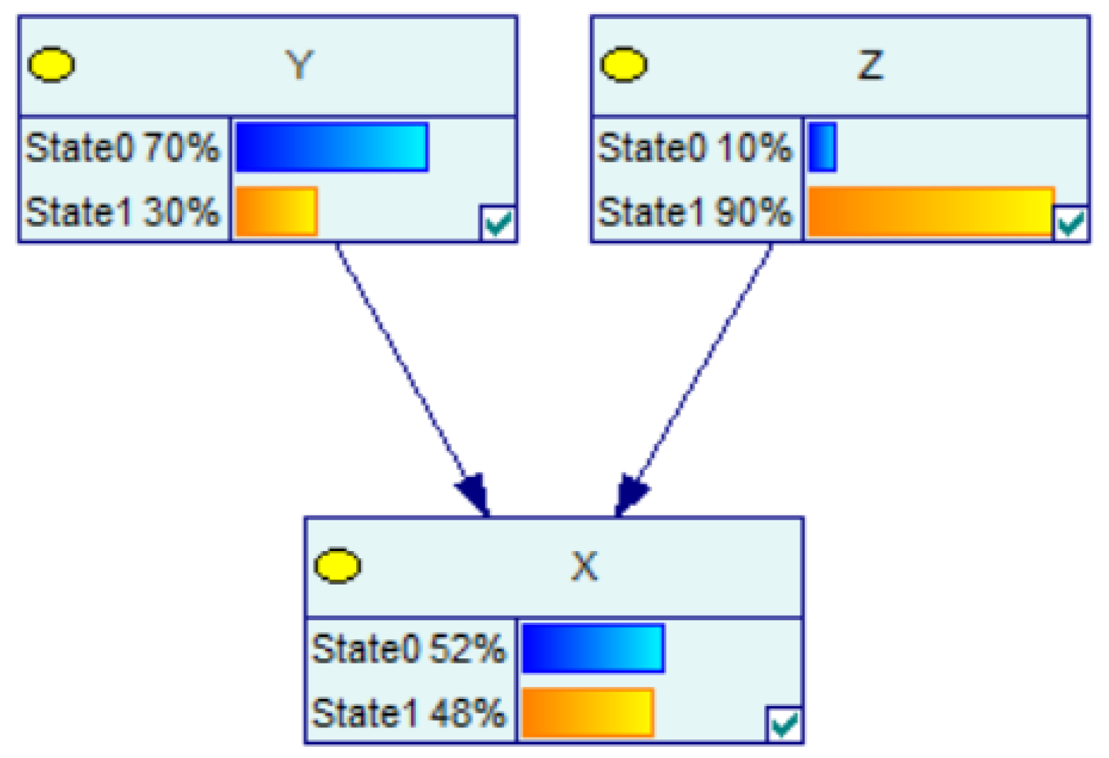
The second algorithm that we propose is the ‘Weighted Diamond’ algorithm. First, both the child state and the parent state have to be ordered. The child state has to be ordered in some relation from most preferred to least preferred. The parent state has to be ordered such that the resulting child state is expected to be decreasing. In practice, this is done by defining some ranking rules, with which the order can be generated automatically. Now, start with the combination of parent states, for which the most preferred child state gets a probability of one, and end with the combination of parent states, for which the least preferred child state gets a probability of one. For the middle one of all the combinations of the parent states, all child states have the same probability $1/M$. Again, we add extra flexibility by not only asking for a ranking of the parent states, but also assigning a relative weight (${\omega }_{i,j}\in {\mathbb{R}}^{+}$), with a higher weight corresponding to a better state and no further scaling needed. Using the same definition for $BS$ and $WS$, we define

$$\begin{array}{c}{\delta }^{\prime }=\frac{1}{2M-2}(BS-WS),\end{array}$$

(15)

$$\begin{array}{c}{\eta }_m^{\prime }=BS-m{\delta }^{\prime }.\end{array}$$

(16)

For the kth combination of parent nodes, we define

$$\begin{array}{cc}\hfill {\mathrm{Score}}_k& =\sum _i{w}_i{P}_{ik},\hfill \end{array}$$

(17)

$$\begin{array}{cc}\hfill {\mathrm{Score}}_k^{\prime }& =|{\mathrm{Score}}_k-\frac{1}{2}(BS+WS)|+\frac{1}{2}(BS+WS).\hfill \end{array}$$

(18)

Now, find the j for which ${\eta }_{j-1}^{\prime }\le {\mathrm{Score}}_k^{\prime }<{\eta }_j^{\prime }$ and calculate:

$$\begin{array}{cc}\hfill P_{j+1}^{\prime }& =\frac{1}{j+1}\frac{{\eta }_{j-1}^{\prime }-{\mathrm{Score}}_k^{\prime }}{-\delta },\hfill \end{array}$$

(19)

$$\begin{array}{cc}\hfill P_m^{\prime }& =(1-P_{j+1}^{\prime })/jm=1,...j.\hfill \end{array}$$

(20)

The last step is calculating the resulting probabilities:

$$\begin{array}{ccc}\hfill P_{m,k}& =P_m^{\prime }\hfill & \hfill \mathrm{if} TS\ge \frac{1}{2}(BS+WS),\end{array}$$

(21)

$$\begin{array}{ccc}\hfill P_{m,k}& =P_{m-j+1}^{\prime }\hfill & \hfill \mathrm{if} TS<\frac{1}{2}(BS+WS).\end{array}$$

(22)

2.4. Example

We now look at an example. Assume that a child node has four states $(Chil{d}_1,...,Chil{d}_4)$ and four parent nodes $(Paren{t}_1,...,Paren{t}_4)$, having four, two, three and four states, respectively. The weights of the parent nodes and the weights of the parent states ($Stat{e}_{XY}$ for state Y of parent X) are depicted in

Table 2. The weights of the parent nodes and the weights of the child states.

	${Parent}_1$	${Parent}_2$	${Parent}_3$	${Parent}_4$
Node weight	0.4	0.25	0.2	0.15
$Stat{e}_{X1}$ weight	2.0	2.0	2.0	2.0
$Stat{e}_{X2}$ weight	1.7	1.0	1.5	1.7
$Stat{e}_{X3}$ weight	1.3	-	1.0	1.3
$Stat{e}_{X4}$ weight	1.0	-	-	1.0

 When we order the states of the system on the score per combination of parent states, the probability per child state can be depicted. This is shown in Figure 5, Figure 6 and Figure 7. Note that despite the weights, the patterns are totally symmetric. The weights have an influence on the order of the combinations of parent states, which influences the probability per combination. The figures show that Hassall’s algorithm spreads the probability over the child nodes with small deviations. In all cases, all child states have a non-zero probability of occurrence. The Weighted Diagonal algorithm indeed gives a value to (at most) two child states at the same time, using the total range from zero to one. The Weighted Diamond algorithm starts (and ends) with full probability on one of the states and has, for the middle combination of parent states, the situation that all states have an equal probability.

Because the definition of the score parameter differs per method, the combinations of parent states are not ordered the same for each method. This is shown in Figure 8, Figure 9 and Figure 10. The given combination is for Hassall’s algorithm a bit left of the middle, and the other two are on the right side of the middle.

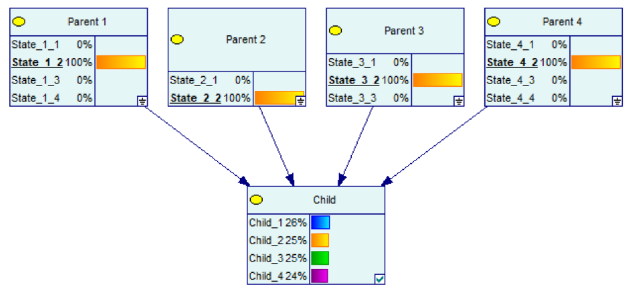
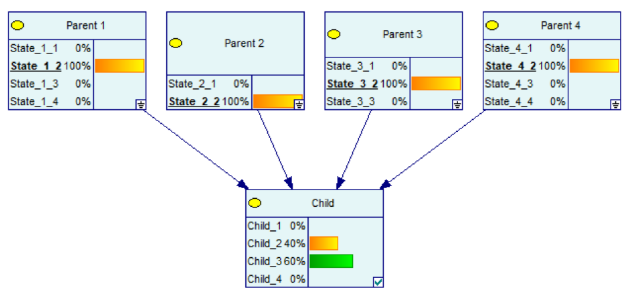
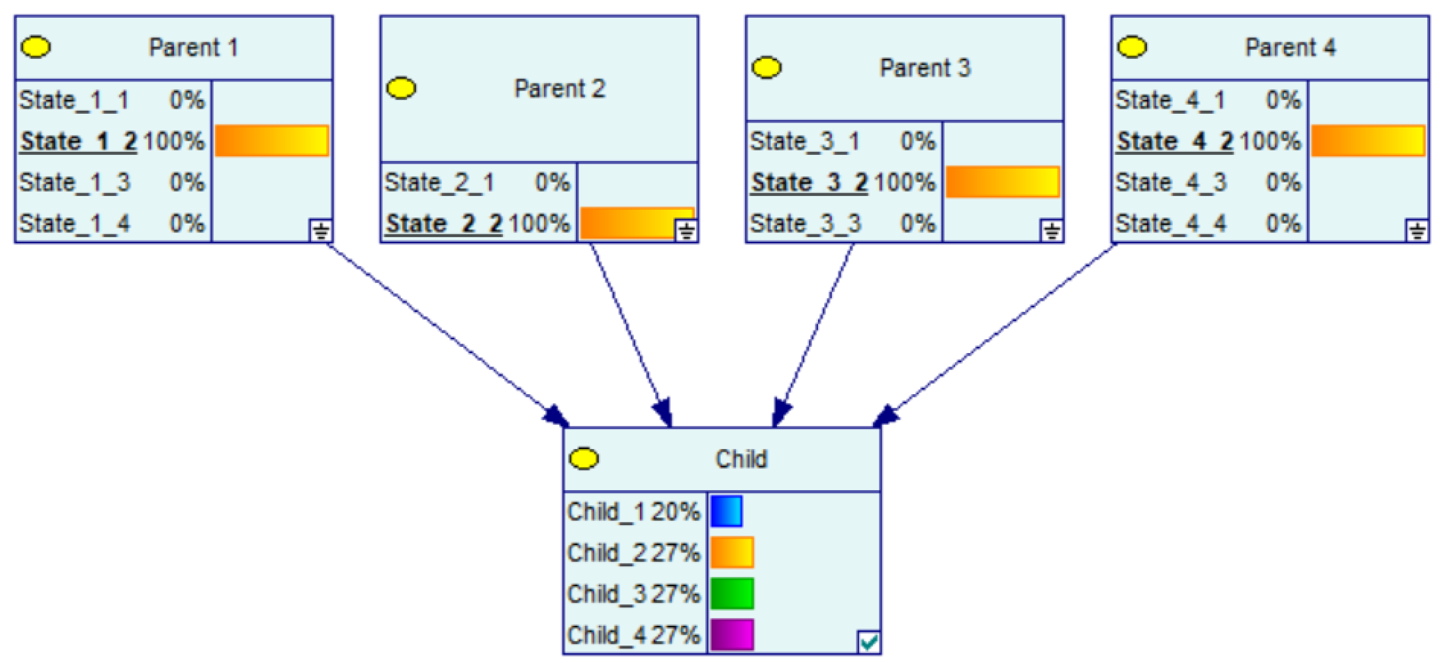
3. CPT Generation Using CPT per Parent

The second approach to generate the CPT for a child with multiple parents is using a CPT per parent and combining these to one generic table. This approach can be used when the influence of a parent, i.e., the CPT per parent, is available or can be generated quite easily and the parents are (supposed) independent of each other. Here also, there are multiple ways to realize this. Again, we have the relative weights of the influence of the parent nodes on the child node ($w_i\in {\mathbb{R}}^{+}$). Now, we assume a given CPT per parent and use $p_{m,i,j}$ to denote the probability of parent i, state j on child state m. Next, we introduce a child state (state M) that stands for ‘NONE’. Now, for a specific combination of parent states $k=\{k_1,...,k_K\}$, we calculate, using the intermediate variables $Z_m$ and $Y_m$:

$$\begin{array}{c}{Z}_m=\sum _{i=1}^K{p}_{m,i,k_i}{w}_{i}m=1,...,M-1,\end{array}$$

(23)

$$\begin{array}{c}{Y}_m=\frac{Z_m}{{\sum }_{i=1}^{M-1}{Z}_i}·\prod _{i=1}^K{\mathbb{1}}_{p_{m,i,k_i}>0}m=1,...,M-1,\end{array}$$

(24)

$$\begin{array}{c}{Y}_M=1-\sum _{m=1}^{M-1}{Y}_m,\end{array}$$

(25)

to obtain the probability for the mth child state, given the kth combination of parent nodes

$$P_{m,k}=Y_m.$$

(26)

This means that we calculate the probabilities of combining the parent states. If a certain combination is not possible, meaning $p_{m,i,j}=0$, this probability mass is assigned to the state ‘NONE’. We will call this method using the ‘NONE’ state for all combinations of parent states that are not possible in the first approach. An alternative, the second approach, is that the probability mass that disappears by a certain $p_{m,i,j}=0$ is redistributed pro rata. Now, state ‘NONE’ is a generic state, leading to

$$P_{m,k}^{\prime }=Y_m^{\prime }=\frac{Z_m}{{\sum }_{i=1}^{M-1}{Z}_i}m=1,...,M.$$

(27)

Example

We look at an example where a certain node has three parents, where each parent has two states and the child has three states and a ’NONE’ state. The conditional probability table of each parent is given in

Table 3. Example CPT for each parent separately.

	Parent 1		Parent 2		Parent 3
State	SP11	SP12	SP21	SP22	SP31	SP32
Node weight	4		4		4
State 1 weight	0.3	0.2	0.2	0.2	0.8	0.0
State 2 weight	0.2	0.6	0.2	0.5	0.2	0.5
State 3 weight	0.5	0.1	0.4	0.0	0.0	0.3
’NONE’ weight	0.0	0.1	0.2	0.3	0.0	0.2

. Here, SP11 stands for State 1 of Parent 1. The resulting CPT for the first approach is shown in

Table 4. Example of the final CPT for the first approach, using the ‘NONE’ state for all combinations of parent states that are not possible.

	SP11						SP12
	SP21			SP22			SP21			SP22
	SP31	SP32		SP31	SP32		SP31	SP32		SP31	SP32
State 1	0.46	0		0.48	0		0.44	0		0.46	0
State 2	0.21	0.35		0.33	0.48		0.37	0.52		0.50	0.67
State 3	0	0.46		0	0		0	0.32		0	0
NONE	0.32	0.19		0.19	0.52		0.19	0.16		0.04	0.33

. See, for example, that the combination $\{\mathrm{SP}11,\mathrm{SP}21,\mathrm{SP}31\}$ has a zero probability for State 3 (Table 4), caused by the zero probability of SP31 on State 3 (Table 3). For the second approach ($P_{m,k}^{\prime }$), the probabilities are listed in

Table 5. Example of the final CPT for the second approach.

	SP11						SP12
	SP21			SP22			SP21			SP22
	SP31	SP32		SP31	SP32		SP31	SP32		SP31	SP32
State 1	0.43	0.17		0.43	0.17		0.40	0.13		0.40	0.13
State 2	0.20	0.30		0.30	0.40		0.33	0.43		0.43	0.53
State 3	0.30	0.40		0.17	0.27		0.17	0.27		0.03	0.13
NONE	0.07	0.13		0.10	0.17		0.10	0.17		0.13	0.20

. Now, the zero-probability entries disappear, as expected.

4. Conclusions

Filling conditional probability tables when working with BBNs can be hard to do, caused by the size of those tables and the necessity of insight into all the relations and dependencies to fill the table in a structured way. Generating standardized starting points, based on limited input, for further use in the elicitation process can help here. Using those processes shows that there is a lot of freedom, where the modeler has to make a choice. Starting from the algorithm by Hassall et al., we proposed two other algorithms to create specific patterns for the CPT. These patterns provide a starting point, based on a small number of parameters, that can be elaborated further in co-operation with domain experts. For when there is more information available, for example a CPT per parent node, we propose another algorithm that creates the full CPT over all parent nodes. Here also, there are many choices that a modeler can exploit. For further research, we recommend to compare the approaches presented in this paper, Wisse et al. [20] and Hassall et al. [21] to the automated entropy-based solutions, like [22].

References

1. Dang, K.B.; Windhorst, W.; Burkhard, B.; Müller, F. A Bayesian Belief Network-Based Approach to Link Ecosystem Functions with Rice Provisioning Ecosystem Services. Ecol. Indic. 2019, 100, 30–44. [Google Scholar] [CrossRef]
2. Zeng, L.; Li, J. A Bayesian belief network approach for mapping water conservation ecosystem service optimization region. J. Geogr. Sci. 2019, 29, 1021–1038. [Google Scholar] [CrossRef] [Green Version]
3. Delen, D.; Topuz, K.; Eryarsoy, E. Development of a Bayesian Belief Network-Based DSS for Predicting and Understanding Freshmen Student Attrition. Eur. J. Oper. Res. 2020, 281, 575–587. [Google Scholar] [CrossRef]
4. Addae, J.H.; Sun, X.; Towey, D.; Radenkovic, M. Exploring user behavioral data for adaptive cybersecurity. User Model. User Adapt. Interact. 2019, 29, 701–750. [Google Scholar] [CrossRef]
5. Sharma, V.K.; Sharma, S.K.; Singh, A.P. Risk enablers modelling for infrastructure projects using Bayesian belief network. Int. J. Constr. Manag. 2019, 1–18. [Google Scholar] [CrossRef]
6. Tang, K.; Parsons, D.J.; Jude, S. Comparison of automatic and guided learning for Bayesian networks to analyse pipe failures in the water distribution system. Reliab. Eng. Syst. Saf. 2019, 186, 24–36. [Google Scholar] [CrossRef]
7. Khakzad, N.; Khan, F.; Amyotte, P. Safety analysis in process facilities: Comparison of fault tree and Bayesian network approaches. Reliab. Eng. Syst. Saf. 2011, 96, 925–932. [Google Scholar] [CrossRef]
8. Kammouh, O.; Gardoni, P.; Cimellaro, G.P. Probabilistic framework to evaluate the resilience of engineering systems using Bayesian and dynamic Bayesian networks. Reliab. Eng. Syst. Saf. 2020, 198, 106813. [Google Scholar] [CrossRef]
9. Falzon, L. Using Bayesian network analysis to support centre of gravity analysis in military planning. Eur. J. Oper. Res. 2006, 170, 629–643. [Google Scholar] [CrossRef]
10. Cao, T.; Coutts, A.; Lui, F. Combined Bayesian belief network analysis and systems architectural approach to analyse an amphibious C4ISR system. In Proceedings of the 22nd National Conference of the Australian Society for Operations Research, Adelaide, Australia, 1–6 December 2013; pp. 1–6. [Google Scholar]
11. Phillipson, F.; Bastings, I.C.; Vink, N. Modelling the Effects of a CBRN Defence System Using a Bayesian Belief Model. In Proceedings of the 9th Symposium on CBRNE Threats—How does the Landscape Evolve? (NBC 2015), Helsinki, Finland, 18–21 May 2015. [Google Scholar]
12. Potter, B.K.; Forsberg, J.A.; Silvius, E.; Wagner, M.; Khatri, V.; Schobel, S.A.; Belard, A.J.; Weintrob, A.C.; Tribble, D.R.; Elster, E.A. Combat-related invasive fungal infections: Development of a clinically applicable clinical decision support system for early risk stratification. Mil. Med. 2019, 184, e235–e242. [Google Scholar] [CrossRef] [PubMed] [Green Version]
13. Arora, P.; Boyne, D.; Slater, J.J.; Gupta, A.; Brenner, D.R.; Druzdzel, M.J. Bayesian Networks for Risk Prediction Using Real-World Data: A Tool for Precision Medicine. Value Health 2019, 22, 439–445. [Google Scholar] [CrossRef] [PubMed] [Green Version]
14. Phillipson, F.; Matthijssen, E.; Attema, T. Bayesian belief networks in business continuity. J. Bus. Contin. Emerg. Plan. 2014, 8, 20–30. [Google Scholar]
15. Lee, H. Design of a BIA and Continuity Strategy in BCMS Using a Bayesian Belief Network for the Manufacturing Industry. J. Korean Soc. Hazard Mitig. 2019, 19, 135–141. [Google Scholar] [CrossRef] [Green Version]
16. Cooke, R. Experts in Uncertainty: Opinion and Subjective Probability in Science; Oxford University Press: Oxford, UK, 1991. [Google Scholar]
17. O’Hagan, A.; Buck, C.E.; Daneshkhah, A.; Eiser, J.R.; Garthwaite, P.H.; Jenkinson, D.J.; Oakley, J.E.; Rakow, T. Uncertain Judgements: Eliciting Experts’ Probabilities; John Wiley & Sons: Chichester, UK, 2006. [Google Scholar]
18. Hanea, A.; McBride, M.; Burgman, M.; Wintle, B.; Fidler, F.; Flander, L.; Twardy, C.; Manning, B.; Mascaro, S. Investigate Discuss Estimate Aggregate for Structured Expert Judgement. Int. J. Forecast. 2017, 33, 267–279. [Google Scholar] [CrossRef]
19. Werner, C.; Bedford, T.; Cooke, R.M.; Hanea, A.M.; Morales-Napoles, O. Expert judgement for dependence in probabilistic modelling: A systematic literature review and future research directions. Eur. J. Oper. Res. 2017, 258, 801–819. [Google Scholar] [CrossRef] [Green Version]
20. Wisse, B.W.; van Gosliga, S.P.; van Elst, N.P.; Barros, A.I. Relieving the Elicitation Burden of Bayesian Belief Networks. In Proceedings of the Sixth UAI Bayesian Modelling Applications Workshop (BMA), Helsinki, Finland, 9 July 2008. [Google Scholar]
21. Hassall, K.L.; Dailey, G.; Zawadzka, J.; Milne, A.E.; Harris, J.A.; Corstanje, R.; Whitmore, A.P. Facilitating the Elicitation of Beliefs for Use in Bayesian Belief Modelling. Environ. Model. Softw. 2019, 122, 104539. [Google Scholar] [CrossRef]
22. Dragos, V.; Ziegler, J.; de Villiers, J.P.; de Waal, A.; Jousselme, A.L.; Blasch, E. Entropy-Based Metrics for URREF Criteria to Assess Uncertainty in Bayesian Networks for Cyber Threat Detection. In Proceedings of the 2019 22th International Conference on Information Fusion (FUSION), Ottawa, ON, Canada, 2–5 July 2019; pp. 1–8. [Google Scholar]
23. Maung, I.; Paris, J.B. A note on the infeasibility of some inference processes. Int. J. Intell. Syst. 1990, 5, 595–603. [Google Scholar] [CrossRef]
24. Holmes, D.E. Innovations in Bayesian Networks: Theory and Applications; Springer: Berlin/Heidelberg, Germany, 2008; Volume 156. [Google Scholar]
Figure 1. Example of a BBN, expressing the marginal probability of X.
Mca 26 00054 g001
Figure 2. Graphical representation of the probability mass distribution of Hassall’s algorithm as a heat map, where a probability of one gives black values and zero white values.
Mca 26 00054 g002
Figure 3. Graphical representation of the probability mass distribution of the Weighted Diagonal algorithm as a heat map, where a probability of one gives black values and zero white values.
Mca 26 00054 g003
Figure 4. Graphical representation of the probability mass distribution of the Weighted Diamond algorithm as a heat map, where a probability of one gives black values and zero white values.
Mca 26 00054 g004
Figure 5. Hassall’s algorithm: the probability per child state, given the ordening of the parents states on the x-axes.
Mca 26 00054 g005
Figure 6. Weighted Diagonal: the probability per child state, given the ordening of the parents states on the x-axes.
Mca 26 00054 g006
Figure 7. Weighted Diamond: the probability per child state, given the ordening of the parents states on the x-axes.
Mca 26 00054 g007
Figure 8. Hassall’s algorithm: example to show the order of the parent’s states.
Mca 26 00054 g008
Figure 9. Weighted Diagonal: example to show the order of the parent’s states.
Mca 26 00054 g009
Figure 10. Weighted Diamond: example to show the order of the parent’s states.
Mca 26 00054 g010