Chaotic Multi-Objective Simulated Annealing and Threshold Accepting for Job Shop Scheduling Problem

Abstract

The Job Shop Scheduling Problem (JSSP) has enormous industrial applicability. This problem refers to a set of jobs that should be processed in a specific order using a set of machines. For the single-objective optimization JSSP problem, Simulated Annealing is among the best algorithms. However, in Multi-Objective JSSP (MOJSSP), these algorithms have barely been analyzed, and the Threshold Accepting Algorithm has not been published for this problem. It is worth mentioning that the researchers in this area have not reported studies with more than three objectives, and the number of metrics they used to measure their performance is less than two or three. In this paper, we present two MOJSSP metaheuristics based on Simulated Annealing: Chaotic Multi-Objective Simulated Annealing (CMOSA) and Chaotic Multi-Objective Threshold Accepting (CMOTA). We developed these algorithms to minimize three objective functions and compared them using the HV metric with the recently published algorithms, MOMARLA, MOPSO, CMOEA, and SPEA. The best algorithm is CMOSA (HV of 0.76), followed by MOMARLA and CMOTA (with HV of 0.68), and MOPSO (with HV of 0.54). In addition, we show a complexity comparison of these algorithms, showing that CMOSA, CMOTA, and MOMARLA have a similar complexity class, followed by MOPSO.

1. Introduction

The Job Shop Scheduling Problem (JSSP) has enormous industrial applicability. This problem consists of a set of jobs, formed by operations, which must be processed in a set of machines subject to constraints of precedence and resource capacity. Finding the optimal solution for this problem is too complex, and so it is classified in the NP-hard class [1,2]. On the other hand, the JSSP foundations provide a theoretical background for developing efficient algorithms for other significant sequencing problems, which have many production systems applications [3]. Furthermore, designing and evaluating new algorithms for JSSP is relevant not only because it represents a big challenge but also for its high industrial applicability [4].

There are several JSSP taxonomies; one of which is single-objective and multi-objective optimization. The single-objective optimization version has been widely studied for many years, and the Simulated Annealing (SA) [5] is among the best algorithms. The Threshold Accepting (TA) algorithm from the same family is also very efficient in this area [6]. In contrast, in the case of Multi-Objective Optimization Problems (MOOPs), both algorithms for JSSP and their comparison are scarce.

Published JSSP algorithms for MOOP include only a few objectives, and only a few performance metrics are reported. However, it is common for the industrial scheduling requirements to have several objectives, and then the Multi-Objective JSSP (MOJSSP) becomes an even more significant challenge. Thus, many industrial production areas require the multi-objective approach [7,8].

In single-objective optimization, the goal is to find the optimal feasible solution of an objective function. In other words, to find the best value of the variables which fulfill all the constraints of the problem. On the other hand, for MOJSSP, the problem is to find the optimum of a set of objective functions $f_1\left(x\right)$, $f_2\left(x\right)\dots f_n\left(x\right)$ depending on a set of variables x and subject to a set of constraints defined by these variables. To find the optimal solution is usually impossible because fulfilling some objective functions may not optimize the other objectives of the problem. In MOOP, a preference relation or Pareto dominance relation produces a set of solutions commonly called the Pareto optimal set [9]. The Decision Makers (DMs) should select from the Pareto set the solution that satisfies their preferences, which can be subjective, based on experience, or will most likely be influenced by the industrial environment’s needs [10]. Therefore, the DM needs to have a Pareto front that contains multiple representative compromise solutions, which exhibit both good convergence and diversity [11].

In the study of single-objective JSSP, many algorithms have been applied. Some of the most common are SA, Genetic Algorithms (GAs), Tabu Search (TS), and Ant Systems (ASs) [12]. In addition, as we mention below, few works in the literature solve JSSP instances with more than two objectives and applying more than two metrics to evaluate their performance. Nevertheless, for MOJSSP, the number of objectives and performance metrics remains too small [8,13,14,15]. The works of Zhao [14] and Mendez [8] are exceptions because the authors have presented implementations with two or three significant objective functions and two performance metrics. Moreover, SA and TA have shown to be very efficient for solving NP-hard problems. Thus, this paper’s motivation is to develop new efficient SA algorithms for MOJSSP with two or more objective functions and a larger number of performance metrics.

The first adaptation of SA to MOOP was an algorithm proposed in 1992, also known as MOSA [16]. An essential part of this algorithm is that it applies the Boltzmann criterion for accepting bad solutions, commonly used in single-objective JSSP. MOSA combines several objective functions. The single-objective JSSP optimization with SA algorithm and MOSA algorithm for multi-objective optimization is different in several aspect related to determining the energy functions, using and generating new solutions, and measuring their quality as is well known, these energy functions are required in the acceptance criterion. Multiple versions of MOSA have been proposed in the last few years. One of them, published in 2008, is AMOSA, that surpassed other MOOP algorithms at this time [17]. In this work, we adapt this algorithm for MOJSSP. TA [6] is an algorithm for single-objective JSSP, which is very similar to Simulated Annealing. These two algorithms have the same structure, and both use a temperature parameter, and they accept some bad solutions for escaping from local optima. In addition, these algorithms are among the best JSSP algorithms, and their performance is very similar. Nevertheless, for MOJSSP, a TA algorithm has not been published, and so for obvious reason, it was not compared with the SA multi-objective version.

MOJSSP has been commonly solved using IMOEA/D [14], NSGA-II [18], SPEA [19], MOPSO [20], and CMOEA [21]; the latter was renamed CMEA in [8]. Nevertheless, the number of objectives and performance metrics of these algorithms remains too small. The Evolutionary Algorithm based on decomposition proposed in 2016 by Zhao in [14] was considered the best algorithm [22]. The Multi-Objective Q-Learning algorithm (MOQL) for JSSP was published in 2017 [23]; this approach uses several agents to solve JSSP. An extension of MOQL is MOMARLA, which was proposed in 2019 by Mendez [8]. This MOJSSP algorithm uses two objective functions: makespan and total tardiness. MOMARLA overcomes the classical multi-objective algorithms SPEA [19], CMOEA [21], and MOPSO [20].

The two new algorithms presented in this paper for JSSP are Chaotic Multi-Objective Simulated Annealing (CMOSA) and Chaotic Multi-Objective Threshold Accepting (CMOTA). The first algorithm is inspired by the classic MOSA algorithm [17]. However, CMOSA is different in three aspects: (1) for the first time it is designed specifically for MOJSSP, (2) it uses an analytical tuning of the cooling scheme parameters, and (3) it uses chaotic perturbations for finding new solutions and for escaping from local optima. This process allows the search to continue from a different point in the solution space and it contributes to a better diversity of the generated solutions. Furthermore, CMOTA is based on CMOSA and Threshold Accepting, and it does not require the Boltzmann distribution. Instead, it uses a threshold strategy for accepting bad solutions to escape from local optima. In addition, a chaotic perturbation function is applied.

In this paper, we present two new alternatives for MOJSSP, and we consider three objective functions: makespan, total tardiness, and total flow time. The first objective is very relevant for production management applications [7], while the other two are critical for enhancing client attention service [23]. In addition, we use six metrics for the evaluation of these algorithms, and they are Mean Ideal Distance (MID), Spacing (S), Hypervolume (HV), Spread ($\Delta$), Inverted Generational Distance (IGD), and Coverage (C). We also apply an analytical tuning parameter method to these algorithms. Finally, we compare the achieved results with those obtained with the JSSP algorithm cited below in [8,14].

The rest of the paper is organized as follows. In Section 2, we make a qualitative comparison of related MOJSSP works. In Section 3, we present MOJSSP concepts and the performance metrics that were applied. Section 4 presents the formulation of MOJSSP with three objectives. The proposed algorithms, their tuning method, and the chaotic perturbation are also shown in Section 5. Section 6 shows the application of the proposed algorithms to a set of 70, 58, and 15 instances. Finally, the results are shown and compared with previous works. In Section 7, we present our conclusions.

2. Related Works

As mentioned above, in single-objective optimization, the JSSP community has broadly investigated the performance of the different solution methods. However, the situation is entirely different for MOJSSP, and there is a small number of published works. In 1994, an analysis of SA family algorithms for JSSP was presented [24]; two of them were SA and TA, which we briefly explain in the next paragraph. These algorithms suppose that the solutions define a set of macrostates of a set of particles, while the objective functions’ values represent their energy, and both algorithms have a Metropolis cycle where the neighborhood of solutions is explored. In single-objective optimization, for the set of instances used to evaluate JSSP algorithms, SA obtained better results than TA. Furthermore, a better solution than the previous one is always accepted, while a worse solution may be accepted depending on the Boltzmann distribution criterion. This distribution is related to the current temperature value and the increment or decrement of energy (associated with the objective functions) in the current temperature value. In the TA case, a worse solution than the previous one may be accepted using a criterion that tries to emulate the Boltzmann distribution. This criterion establishes a possible acceptance of a worse solution when the decrement of energy is smaller than a threshold value depending on the temperature and a parameter $\gamma$ that is very close to one. Then at the beginning of the process, the threshold values are enormous because they depend on the temperatures. Subsequently, the temperature parameter is gradually decreased until a value close to zero is achieved, and then this threshold is very small.

In 2001, a Multi-Objective Genetic Algorithm was proposed to minimize the makespan, total tardiness, and the total idle time [25]. The proposed methodology for JSSP was assessed with 28 benchmark problems. In this publication, the authors randomly weighted the different fitness functions to determine their results.

In 2006, SA was used for two objectives: the makespan and the mean flow time [26]. This algorithm was called Pareto Archived Simulated Annealing (PASA), which used the Simulated Annealing algorithm with an overheating strategy to escape from local optima and to improve the quality of the results. The performance of this algorithm was evaluated with 82 instances taken from the literature. Unfortunately, this method has not been updated for three or more objective functions.

In 2011, a two-stage genetic algorithm (2S-GA) was proposed for JSSP with three objectives to minimize the makespan, total weighted earliness, and total weighted tardiness [13]. In the first stage, a parallel GA found the best solution for each objective function. Then, in the second stage, the GA combined the populations, which evolved using the weighted aggregating objective function.

Researchers from the Contemporary Design and Integrated Manufacturing Technology (CDIMT) laboratory proposed an algorithm named Improved Multi-Objective Evolutionary Algorithm based on Decomposition (IMOEA/D) to minimize the makespan, tardiness, and total flow time [14]. The authors experiment with 58 benchmark instances, and they use the performance metrics Coverage [27] and Mean Ideal Distance (MID) [28] to evaluate their algorithm. We notice in

Table 1. Related Works.

Algorithm	Objectives	Metrics
SA [16]	Makespan	*
SA and TA [24]	Makespan	*
Hybrid GA [25]	Makespan, total tardiness, and total idle time	*
PASA [26]	Makespan, mean flow time	*
2S-GA [13]	Makespan, total weighted earliness, and  total weighted tardiness	*
IMOEA/D [14]	Makespan, total flow time, and tardiness time	C, MID
Hybrid GA/LS/LP [15]	Weighted tardiness, and energy costs	HV
MOMARLA [8]	Makespan, total tardiness	HV
CMOSA and CMOTA (This paper)	Makespan, total tardiness, and total flow time	MID, S, HV, $\Delta$, IGD and C

* Not reported.

, studies with two or three objectives, but they do not report any metric. On the other hand, IMOEA/D stands out from the rest of the literature, not only because the authors reported good results but also because they considered a more significant number of objectives, and they applied two metrics.

In 2008, the AMOSA algorithm based on SA for several objectives was proposed [17]. In this paper, the authors reported that the AMOSA algorithm performed better than some MOEA algorithms, one of them NSGA-II [29]. They presented the main Boltzmann rules for accepting bad solutions. Unfortunately, a MOJSSP with AMOSA and with more than two objectives has not been published.

In 2017, a hybrid algorithm between an NSGA-II and a linear programming approach was proposed [15]; it was used to solve the FT10 instance of Taillard [30]. This algorithm minimized the weighted tardiness and energy costs. To evaluate the performance, the authors only used the HV metric.

In 2019, MOMARLA was proposed, a new algorithm based on Q-Learning to solve MOJSSP [8]. This work provided flexibility to use decision-maker preferences; each agent represented a specific objective and used two action selection strategies to find a diverse and accurate Pareto front. In Table 1, we present the last related studies for MOJSSP and the proposed algorithms.

This paper analyzes our algorithms CMOSA and CMOTA, as follows: (a) comparing CMOSA and CMOTA versus IMOEA/D [14], (b) comparing our algorithms with the results published for MOMARLA, MOPSO, CMOEA, and SPEA, and (c) comparing CMOSA versus CMOTA.

3. Multi-Objective Optimization

In a single-objective problem, the algorithm finishes its execution when it finds the solution that optimizes the objective function or a very close optimal solution. However, for Multi-Objective Optimization, the situation is more complicated since several objectives must be optimized simultaneously. Then, it is necessary to find a set of solutions optimizing each of the objectives individually. These solutions can be contrasting because we can obtain the best solution for an objective function that is not the best for other objective functions.

3.1. Concepts

Definitions of some concepts of Multi-Objective Optimization are shown below.

Pareto Dominance: In general, for any optimization problem, solution A dominates another solution B if the following conditions are met [31]: A is strictly better than B on at least one objective, and A is not worse than B for any objective function.

Non-dominated set: In a set of P solutions, the non-dominated solutions P1 is integrated by solutions that accomplish the following conditions [31]: any pair of P1 solutions must be non-dominated (one regarding the other), and any solution that does not belong to P1 is dominated by at least one member of P1.

Pareto optimal set: The set of non-dominated solutions of the total search space.

Pareto front: The graphic representation of the non-dominated solutions of the multi-objective optimization problem.

3.2. Performance Metrics

In an experimental comparison of different optimization techniques or algorithms, it is always necessary to have the notion of performance. In the case of Multi-Objective Optimization, the definition of quality is much more complicated than for single-objective optimization problems because the multi-objective optimization criteria itself consists of multiple objectives, of which, the most important are:

• To minimize the distance of the resulting non-dominated set to the true Pareto front.
• To achieve an adequate distribution (for instance, uniform) of the solutions is desirable.
• To maximize the extension of the non-dominated front for each of the objectives. In other words, a wide range of values must be covered by non-dominated solutions.

In general, it is difficult to find a single performance metric that encompasses all of the above criteria. In the literature, a large number of performance metrics can be found. The most popular performance metrics were used in this research and are described below:

Mean Ideal Distance: Evaluates the closeness of the calculated Pareto front ($P{F}_{calc}$) solutions with an ideal point, which is usually (0, 0) [28].

$$MID=\frac{{\sum }_{i=1}^Q{c}_i}{Q}$$

(1)

where $c_i=\sqrt{f_{1,i}^2+f_{2,i}^2+f_{3,i}^2}$ and $f_{1,i},f_{2,i},f_{3,i}$ are the values of the i-th non-dominated solution for their first, second, and third objective function, and Q is the number of solutions in the $P{F}_{calc}$.

Spacing: Evaluates the distribution of non-dominated solutions in the $P{F}_{calc}$. When several algorithms are evaluated with this metric, the best is that with the smallest S value [32].

$$S=\sqrt{\frac{{\sum }_{i=1}^Q{(d_i-\overline{d})}^2}{Q}}$$

(2)

where $d_i$ measures the distance in the space of the objective functions between the i-th solution and its nearest neighbor; that is the j-th solution in the $P{F}_{calc}$ of the algorithm, Q is the number of the solutions in the $P{F}_{calc}$, $\overline{d}$ is the average of the $d_i$, that is $\overline{d}={\sum }_{i=1}^Q\frac{d_i}{Q}$ and $d_i=mi{n}_j\left(\right|f_1^i\left(x\right)-f_1^j\left(x\right)|+|f_2^i\left(x\right)-f_2^j\left(x\right)|+\dots +|f_M^i\left(x\right)-f_M^j\left(x\right)\left|\right)$, where $f_1^i,f_2^i$ are the values of the i-th non-dominated solution for their first and second objective function, $f_1^j,f_2^j$ are the values of the j-th non-dominated solution for their first and second objective function respectively, M is the number of objective functions and $i,j=1,\dots Q$.

Hypervolume: Calculates the volume in the objective space that is covered by all members of the non-dominated set [33]. The $HV$ metric is measured based on a reference point (W), and this can be found simply by constructing a vector with the worst values of the objective function.

$$HV=volume\left({\cup }_{i=1}^{\left|Q\right|}{v}_i\right)$$

(3)

where $v_i$ is a hypercube and is constructed with a reference point W and the solution i as the diagonal corners of the hypercube [31]. An algorithm that obtains the largest $HV$ value is better. The data should be normalized by transforming the value in the range [0, 1] for each objective separately to perform the calculation.

Spread: This metric was proposed to have a more precise coverage value and considers the distance to the (extreme points) of the true Pareto front ($P{F}_{true}$) [29].

$$\Delta =\frac{{\sum }_{k=1}^M{d}_k^e+{\sum }_{i=1}^Q|d_i-\overline{d}|}{{\sum }_{k=1}^M{d}_k^e+Q\times \overline{d}}$$

(4)

where $d_k^e$ measures the distance between the “extreme” point of the $P{F}_{true}$ for the k-th objective function, and the nearest point of $P{F}_{calc}$, $d_i$ corresponds to the distance between the solution i-th of the $P{F}_{calc}$, while its nearest neighbor, $\overline{d}$ corresponds to the average of the $d_i$ and M is the number of objectives.

Inverted Generational Distance: It is an inverted indicator version of the Generational Distance (GD) metric, where all the distances are measured from the $P{F}_{true}$ to the $P{F}_{calc}$ [1].

$$IGD\left(Q\right)=\frac{{\left({\sum }_{j=1}^{\left|T\right|}{\widehat{d}}_j^p\right)}^{1/p}}{\left|T\right|}$$

(5)

where $T=\{t_1,t_2,\dots ,t_{\left|T\right|}\}$ that is, the solutions in the $P{F}_{true}$ and $\left|T\right|$ is the cardinality of T, p is an integer parameter, in this paper $p=2$ and ${\widehat{d}}_j$ is the Euclidean distance from $t_j$ to its nearest objective vector q in Q, according to (6).

$$d_j=\underset{q=1}{\overset{\left|Q\right|}{min}}\sqrt{\sum _{m=1}^M{(fm\left(t_j\right)-fm\left(q\right))}^2}$$

(6)

where $fm\left(t\right)$ is the m-th objective function value of the t-th member of T and M is the number of objectives.

Coverage: Represents the dominance between set A and set B [27]. It is the ratio of the number of solutions in set B that were dominated by solutions in set A and the total number of solutions in set B. The C metric is defined by (7).

$$C(A,B)=\frac{\left|\right\{b\in B|\exists a\in A:a⪯b\}|}{\left|B\right|}$$

(7)

When $C(A,B)=1$, all B solution are dominated or equal to solutions in A. Otherwise, $C(A,B)=0$, represents situations in which none of the solutions in B is dominated by any solution in A. The higher the value of $C(A,B)$, the more solutions in B are dominated by solutions in A. Both $C(A,B)$ and $C(B,A)$ should be considered, since $C(B,A)$ is not necessarily equal to $1-C(A,B)$.

4. Multi-Objective Job Shop Scheduling Problem

In JSSP, there are a set of n different jobs consisting of operations that must be processed in m different machines. There are a set of precedence constraints for these operations, and there are also resource capacity constraints for ensuring that each machine should process only one operation at the same time. The processing time of each operation is known in advance. The objective of JSSP is to determine the sequence of the operations in each machine (the start and finish time of each operation) to minimize certain objective functions subject to the constraints mentioned above. The most common objective is the makespan, which is the total time in which all the problem operations are processed. Nevertheless, real scheduling problems are multi-objective, and several objectives should be considered simultaneously.

The three objectives that are addressed in the present paper are:

Makespan: the maximum time of completion of all jobs.

Total tardiness: it is calculated as the total positive differences between the makespan and the due date of each job.

Total flow time: it is the summation of the completion times of all jobs.

The formal MOJSSP model can be formulated as follows [34,35]:

$$OptimizeF\left(x\right)=[f_1\left(x\right),f_2\left(x\right),\dots ,f_q\left(x\right)]Subjectto:x\in S$$

(8)

where q is the number of objectives, x is the vector of decision variables, and S represents the feasible region. Defined by the next precedence and capacity constraints, respectively:

$$\begin{array}{ll}{t}_j\ge t_i+p_i& \mathrm{For} \mathrm{all} i,j\in O \mathrm{when} i \mathrm{precedes} j\\ t_j\ge t_i+p_i \mathrm{or} t_i\ge t_j+p_i& \mathrm{For} \mathrm{all} i,j\in O \mathrm{when} M_i=M_j\end{array}$$

where

• $t_i$, $t_j$ are the starting times for the jobs i, $j\in J$.
• $p_i$ and $p_j$ are the processing times for the jobs i, $j\in J$.
• $J:\{J_1,J_2,J_3,\dots ,J_n\}$ it is the set of jobs.
• $M:\{M_1,M_2,M_3,\dots ,M_m\}$ it is the set of machines.
• O is the set of operations $O_{j,i}$ (operation i of the job j).

The objective functions of makespan, total tardiness, and total flow time, are defined by Equations (9)–(11), respectively.

$$f_1=min\left(\underset{j=1}{\overset{n}{max}}{C}_j\right)$$

(9)

where $C_j$ is the makespan of job j.

$$f_2=min\left(\sum _{j=1}^n{T}_j\right)=min\left(\sum _{j=1}^{n}max(0,C_j-D_j)\right)$$

(10)

where $T_j=max(0,C_j-D_j)$ is the tardiness of job j, and $D_j$ is the due date of job j and is calculated with $D_j=\tau {\sum }_{i=1}^m{p}_{j,i}$ [36], where $p_{j,i}$ is the time required to process the job j in the machine i. In this case, the due date of the j job is the sum of the processing time of all its operations on all machines, multiplied by a narrowing factor ($\tau$), which is in the range $1.5\le \tau \le 2.0$ [14,36].

$$f_3=min\sum _{j=1}^n{C}_j$$

(11)

5. Multi-Objective Proposed Algorithms

The two multi-objective algorithms presented in this section for solving JSSP are Chaotic Multi-Objective Simulated Annealing and Chaotic Multi-Objective Threshold Accepting. We describe these algorithms in this section after analyzing the single-objective optimization algorithms for JSSP.

5.1. Simulated Annealing

The algorithm SA proposed by Kirkpatrick et al. comes from a close analogy with the metal annealing process [5]. This process consists of heating and progressively cooling metal. As the temperature decreases, the molecules’ movement slows down and tends to adopt a lower energy configuration. Kirkpatrick et al. proposed this algorithm for combinatorial optimization problems and to escape from local minima. It starts with an initial solution and generates a new solution in its neighborhood. If the new solution is better than the old solution, then it is accepted. Otherwise, SA applies the Boltzmann distribution, which determines if a bad solution can be taken as a strategy for escaping from local optima. This process is repeated many times until an equilibrium condition is accomplished.

The SA algorithm is shown in Algorithm 1. Line 1 receives the parameters: the initial ($T_{initial}$) and final ($T_{final}$) temperatures, the alpha value ($\alpha$) for decreasing the temperature, and beta ($\beta$) for increasing the length of the Metropolis cycle. The current temperature ($T_k$) is set in line 2. An initial solution ($s_{current}$) is generated randomly in line 3. The stop criterion is evaluated (line 4); this main cycle is repeated while the current temperature ($T_k$) is higher than the final temperature ($T_{final}$). The Metropolis cycle starts in line 5, where a neighboring solution ($s_{new}$) is generated (line 6). In line 7 the increment $\Delta E$ of the objective function is determined for the current solution ($s_{current}$) and the new one ($s_{new}$). When this increment is negative (line 8) the new solution is the best. In this case, the new solution replaces the current solution (line 9). Otherwise, the Boltzmann criterion is applied (lines 11 and 12). This criterion allows the algorithm to escape from local optima depending on the current temperature and delta values. Finally, line 16 increases the number of iterations of the Metropolis cycle, and in line 17, the cooling function is applied to reduce the current temperature.

Algorithm 1 Classic Simulated Annealing algorithm
1:	procedureSA($T_{initial},T_{final},\alpha ,\beta ,L_k$)
2:	$T_k\leftarrow T_{initial}$
3:	$s_{current}\leftarrow RandomInitialSolution\left(\right)$
4:	while $T_k\ge T_{final}$ do
5:	for 1 to $L_k$ do
6:	$s_{new}\leftarrow perturbation\left(s_{current}\right)$
7:	$\Delta E\leftarrow E\left(s_{new}\right)-E\left(s_{current}\right)$
8:	if $\Delta E<0$ then
9:	$s_{current}\leftarrow s_{new}$
10:	else
11:	if $(e^{-\Delta E/T_k}>random(0,1)$ then
12:	$s_{current}\leftarrow s_{new}$
13:	end if
14:	end if
15:	end for
16:	$L_k\leftarrow \beta \times L_k$
17:	$T_k\leftarrow \alpha \times T_k$
18:	end while
19:	return $s_{current}$
20:	end procedure

5.2. Analytical Tuning for Simulated Annealing

The parameters tuning process for the SA algorithm used in this paper is based on a method proposed in [37]. This method establishes that both the initial and final temperatures are functions of the maximum and minimum energy values $E_{max}$ and $E_{min}$, respectively. These energies appeared in the Boltzmann distribution criterion that states that a bad solution is accepted in a temperature T when $random(0,1)\le e^{-\Delta E/T}$. For JSSP, $\Delta E$ is obtained with the makespan. For this tuning method, these two functions are obtained from the neighborhood of different solutions randomly generated. A set of previous SA executions must be carried out for obtaining $\Delta E_{max}$ and $\Delta E_{min}$. These value are used in the Boltzmann distribution for determining the initial and final temperatures. Then, the other parameters of Metropolis cycle are determined. The process used is detailed in the next paragraph.

Initial temperature ($T_{initial}$): It is the temperature value from which the search process begins. The probability of accepting a new solution is almost 1 at high temperatures so, its cost of deterioration is maximum. The initial temperature is associated with the maximum allowed deterioration and its defined acceptance probability. Let us define $s_i$ as the current solution, $s_j$ a new proposed solution, $E_{\left(s_i\right)}$ and $E_{\left(s_j\right)}$ are its associated costs, the maximum and minimum deterioration are $\Delta E_{max}$ and $\Delta E_{min}$. Then $P(\Delta E_{max})$, is the probability of accepting a solution with the maximum deterioration and it is calculated with (12). Thus the value of the initial temperature $\left(T_{initial}\right)$ is calculated with (13).

$$P(\Delta E_{max})=e^{(\Delta E_{max}/T_{initial})}$$

(12)

$$T_{initial}=\frac{-\Delta E_{max}}{ln\left(P(\Delta E_{max})\right)}$$

(13)

Final temperature ($T_{final}$): It is the temperature value at which the search stops. In the same way, the final temperature is determined with (14) according to the probability $P(\Delta E_{min})$, which is the probability of accepting a solution with minimum deterioration.

$$T_{final}=\frac{-\Delta E_{min}}{ln\left(P(\Delta E_{min})\right)}$$

(14)

Alpha value ($\alpha$): It is the temperature decrease factor. This parameter determines the speed at which the decrease in temperature will occur, for fast decrements 0.7 it is usually used and for slow decrements 0.99.

Cooling scheme: This function specifies how the temperature is decreased. In this case, the value of the current temperature $\left(T_k\right)$ follows the geometric scheme (15).

$$T_{k+1}=\alpha T_k$$

(15)

Length of the Markov chain or iterations in Metropolis cycle ($L_k$): This refers to the number of iterations of the Metropolis cycle that is performed at each temperature k, this number of iterations can be constant or variable. It is well known that at high temperatures, only a few iterations are required since the stochastic equilibrium is rapidly reached [37]. However, at low temperatures, a much more exhaustive level of exploration is required. Thus, a larger $L_k$ value must be used. If $L_{min}$ is the value of $L_k$ at the initial temperature, and $L_{max}$ is the $L_k$ at the final temperature, then the Formula (16) is used.

$$L_{k+1}=\beta L_k$$

(16)

where $\beta$ is the increment coefficient of $L_k$. Since the Functions (15) and (16) are applied successively in SA from the initial to the final temperature, $T_{final}$ and $L_{max}$ are calculated with (17) and (18).

$$T_{final}={\alpha }^n{T}_{initial}$$

(17)

$$L_{max}={\beta }^n{L}_{min}$$

(18)

In (17) and (18) n is the number of steps from $T_{initial}$ to $T_{final}$, then (19) and (20) are obtained.

$$n=\frac{ln\left(T_{final}\right)-ln\left(T_{initial}\right)}{ln\left(\alpha \right)}$$

(19)

$$\beta =e^{\left(\frac{ln\left(L_{max}\right)-ln\left(L_{min}\right)}{n}\right)}$$

(20)

The probability of selecting the solution $s_j$ from N random samples in the neighborhood $V_{si}$ is given by (21); and from this equation, the N value is obtained in (22), where the exploration level C is defined in Equation (23).

$$P\left(S_j\right)=1-e^{\frac{-N}{\mid V_{si}\mid }}$$

(21)

$$N=-\mid V_{si}\mid ln(1-P\left(S_j\right))=C\mid V_{si}\mid$$

(22)

$$C=ln\left(P\left(S_j\right)\right)$$

(23)

The length of the Markov chain or iterations of the Metropolis cycle are defined by (24).

$$L_{max}=N=C\mid V_{si}\mid$$

(24)

To guarantee a good exploration level, the C value determined by (23) must be established between $1\le C\le 4.6$ [38].

5.3. Chaotic Multi-Objective Simulated Annealing (CMOSA)

As we previously mentioned, the AMOSA algorithm was proposed in [17]. However, this algorithm is designed for general purposes. In this work, we adapt the AMOSA for JSSP to include the following features: (1) the mathematical constraints of MOJSSP, and (2) the objective functions makespan, total tardiness, and total flow time.

CMOSA has the same features previously described and has the next three elements: (1) a new structure, (2) chaotic perturbation, and (3) apply dominance to select solutions. These elements are described in the next subsections.

5.3.1. CMOSA Structure

The CMOSA algorithm uses a chaotic phase to improve the quality of the solutions considering the three objectives. Algorithm 2 receives its parameters in line 1: initial temperature ($T_{initial}$), final temperature ($T_{final}$), alpha ($\alpha$), beta ($\beta$), Metropolis iterations in every cycle ($L_k$), and the initial solution ($s_{current}$) to be improved. In lines 2 and 3, the variables of the algorithm are initialized. In line 4, the $s_{current}$ is processed to obtain the values for each of the three objectives as output. In line 5, the initial temperature is established as the current temperature ($T_k$). Then the main cycle begins in line 6. This cycle is repeated as long as the current temperature is greater than, or equal to, the final temperature. In line 7, the Metropolis cycle begins. Subsequently, the algorithm verifies if it is stagnant in line 8. If that is the case, lines 9 to 20 are executed. The number of iterations to perform a local search is established in line 10; this value is based on the number of tasks of the instance multiplied by an experimentally tuned parameter (in this case, this parameter is $timesLS=10$).

Algorithm 2 Chaotic Multi-Objective Simulated Annealing (CMOSA)
1: procedure CMOSA($T_{initial},T_{final},\alpha ,\beta ,L_k,s_{current}$)
2:    $MAXSTAGNANT\leftarrow 10,counterTrapped\leftarrow 0,isCaught\leftarrow FALSE$
3:    $iterationsLocalSearch\leftarrow tasks\times timesLS,verifyCaught\leftarrow TRUE,countCaught\leftarrow 0$
4:    $mk{s}_{current},td{s}_{current},fl{t}_{current}\leftarrow calculateValues\left(s_{current}\right)$	$▹mks:makespan,tds:tardiness,flt:flowtime$
5:    $T_k\leftarrow T_{initial}$
6:    while $T_k\ge T_{final}$ do
7:        for $i\leftarrow 0$ to $L_k$ do
8:           if $isCaught=TRUE$ then
9:               $isCaught\leftarrow FALSE$
10:               for $k\leftarrow 0$ to $iterationsLocalSearch$ do
11:                   if $k=0$ then
12:                       $s_{new}\leftarrow chaoticPerturbation\left(s_{current}\right)$	▹See Algorithm 4
13:                   else
14:                       $s_{new}\leftarrow regularPerturbation\left(s_{current}\right)$	▹Exchange of two operations
15:                   end if
16:                   $mk{s}_{new},td{s}_{new},fl{t}_{new}\leftarrow calculateValues\left(s_{new}\right)$
17:                   if $(mk{s}_{new}<mk{s}_{current})$ AND $(td{s}_{new}<td{s}_{current})$ AND $(fl{t}_{new}<fl{t}_{current})$ then
18:                       $s_{current}\leftarrow s_{new}$
19:                   end if
20:               end for
21:           else
22:               $s_{new}\leftarrow regularPerturbation\left(s_{current}\right)$
23:               $mk{s}_{new},td{s}_{new},fl{t}_{new}\leftarrow calculateValues\left(s_{new}\right)$
24:           end if
25:           if $(mk{s}_{new}\ne mk{s}_{current})$ AND $(td{s}_{new}\ne td{s}_{current})$ AND $(fl{t}_{new}\ne fl{t}_{current})$ then
26:               $verifyDominanceCMOSA(T_k,s_{new},s_{current})$	▹See Algorithm 5
27:           end if
28:        end for
29:        if $verifyCaught=TRUE$ then
30:           if $caught(s_{current},counterTrapped)=TRUE \mathbf{then}$	▹See Algorithm 3
31:               $countCaught=countCaught+1$
32:               if $countCaught=MAXSTAGNANT$ then
33:                   $verifyCaught\leftarrow FALSE$
34:               end if
35:           end if
36:        end if
37:        $L_k\leftarrow \beta \times L_k$
38:        $T_k\leftarrow \alpha \times T_k$
39:    end while
40:    return $s_{current}$
41: end procedure

In line 11, a local search begins. In the first iteration of this search, a chaotic perturbation (explained in Algorithm 4) is applied to the $s_{current}$ (line 12) to restart the search process from another point in the solution space. In further iterations, a regular perturbation is applied (line 14) that consists only of exchanging the position of two operations in the solution, always verifying that the solution generated is feasible. In line 16, the $s_{new}$ is processed to obtain the values for each of the three objectives. Subsequently, and only if the new solution dominates the current solution of the three objectives, the new solution is used to continue the search process (lines 17 and 18). When the algorithm is not stagnant, a regular perturbation is applied, and the flow continues (line 22). If the current and the new solution are different, we proceed with the dominance verification process to determine which solution is used to continue the search (line 26); this process is explained in Algorithm 5. Finally, from lines 29 to 36, a process is applied to set a limit to the number of times the algorithm is stagnant (See Algorithm 3). The algorithm is determined to be stagnant if, after some iterations, it fails to generate a new, non-dominated solution. In this algorithm, the stagnation is limited to 10 iterations. At the end of the algorithm, in line 37, the number of repetitions of the Metropolis cycle ($L_k$) is increased by multiplying its previous value by the $\beta$ parameter value. Additionally, in line 38, the current temperature ($T_k$) is decreased by multiplying it by the $\alpha$ value. At the end of line 40, the stored solution ($s_{current}$) is generated as the output of the algorithm.

Algorithm 3 shows the process that is carried out to verify the stagnation mentioned in line 30 of Algorithm 2.

Algorithm 3 Caught

1: procedure caught($s_{current},counterTrapped$)

2:    $isCaught\leftarrow FALSE,timesDominated\leftarrow 0,maxTrapped\leftarrow 10$

3:    $timesDominated\leftarrow countTimesDominated\left(s_{current}\right)$

4:    if $timesDominated=0$ then

5:        $F\leftarrow s_{current}$

6:    end if

7:    if $timesDominated\ge 1$ then

8:        $counterTrapped\leftarrow counterTrapped+1$

9:    end if

10:    if $counterTrapped=maxTrapped$ then

11:        $isCaught\leftarrow TRUE$

12:        $counterTrapped\leftarrow 0$

13:    end if

14:    return $isCaught$

15: end procedure

In this Algorithm 3 the current solution ($s_{current}$) and the counter of times it has trapped ($counterTrapped$) are received as input. In line 2 the variables used are initialized. Then the times that the current solution is dominated by at least one solution from the non-dominated front are counted (line 3). If the current solution is non-dominated (line 4) it is stored in the front of non-dominated solutions (line 5). If the current solution is dominated by at least one solution (line 7) then the $counterTrapped$ is incremented (line 8). When $counterTrapped$ equals the maximum number of trapped allowed (line 10), the value of $isCaught$ is set to $TRUE$ (line 11) and the trap counter is reset to zero in line 12.

5.3.2. Chaotic Perturbation

The logistic equation or logistic map is a well-known mathematical application of the biologist Robert May for a simple demographic model [39]. This application tells us the population in the n-th generation based on the size of the previous generation. This value may be found by a popular logistic model mathematically expressed as:

$$x_{n+1}=r{x}_n(1-x_n)$$

(25)

In Equation (25), the variable $x_n$ takes values ranged between zero and one. This variable represents the fraction of individuals in a specific situation (for instance, into a territory or with a particular feature) in a given instant n. The parameter r is a positive number representing the combined ratio between reproduction and mortality. Even though we are not interested in this paper in demographic or similar problems, we notice the very fast last variable changes. Then it can be taken as a chaotic variable. Thus, we use this variable for performing a chaotic perturbation function, which may help to escape from local optima for our CMOTA and CMOSA algorithms.

The chaotic function used is very sensitive to changes in the initial conditions, and this characteristic is used to generate a perturbation to the solution for escaping from local optima. Then chaos or chaotic perturbation is a process carried out to restart the search from another point in the space of solutions.

Algorithm 4 can be explained in three steps. Firstly, the feasible operations (operations that can be performed without violating any restrictions) are searched (line 4). Secondly, whether there is only one feasible operation (line 5) means that it is the last operation and selected (line 6). When there is more than one feasible operation, a chaotic function is applied to select the operations. In this case, the logistic function is used (lines 8–19), which applies a threshold in the range [0.5 to 1]. Finally, the selected operation is added to the new solution (line 21). This process is applied until all the operations are selected.

Algorithm 4 Chaotic perturbation

1: procedure chaoticPerturbation($s_{current}$)

2:    $feasibleTasksNumber\leftarrow 0,r\leftarrow 4,repeat\leftarrow TRUE,X_n\leftarrow 0,X_{n1}\leftarrow 0$

3:    while $counter<tasks$ do

4:        $feasibleTasksNumber\leftarrow searchFeasibleTasks\left(\right)$

5:        if $feasibleTasksNumber=1$ then

6:           $index\leftarrow 0$

7:        else

8:           while $repeat=TRUE$ do

9:               $X_n\leftarrow random(0,1)$

10:               for $i\leftarrow 0$ to $feasibleTasksNumber$ do

11:                   $X_{n1}\leftarrow (r\times X_n)\times (1.0-X_n)$

12:                   if $X_{n1}>0.5$ then

13:                       $index\leftarrow i$

14:                       $repeat\leftarrow FALSE$

15:                       $break$

16:                   end if

17:                   $X_n\leftarrow X_{n1}$

18:               end for

19:           end while

20:        end if

21:        $s_{new}\leftarrow addTask\left(index\right)$

22:        $counter\leftarrow counter+1$

23:    end while

24:    return $s_{new}$

25: end procedure

5.3.3. Applying Dominance to Select Solutions

In Algorithm 5, the current solution ($s_{current}$) is compared with the new solution ($s_{new}$) to determine which solution is used to continue the search. In this comparison, there are three cases:

• If $s_{new}$ dominates $s_{current}$, then $s_{new}$ is used to continue the search (lines 3 to 6).
• If $s_{new}$ is dominated by $s_{current}$ then the differences of each objective are calculated separately from the two solutions compared to obtain the decreased parameter ($\Delta$) and use it to determine if the $s_{new}$ continues with the search according to the condition in line 12. In this case, $s_{current}$ is added to the non-dominated front (F) and $s_{new}$ replaces $s_{current}$ (lines 13 and 14).
• If the two solutions are non-dominated by each other, then the current solution $s_{current}$ is added to the non-dominated front (F), and the search continues with $s_{new}$ (lines 18 to 21).

Algorithm 5: Verify dominance CMOSA

1:procedureverifyDominanceCMOSA($T_k,s_{new},s_{current},mk{s}_{new},td{s}_{new},fl{t}_{new},mk{s}_{current},td{s}_{current},fl{t}_{current}$)

2:    $newDominateCurrent\leftarrow FALSE,currentDominateNew\leftarrow FALSE$

3:    if $s_{new}\prec s_{current}$ then

4:        $s_{current}\leftarrow s_{new}$

5:        $newDominateCurrent\leftarrow TRUE$

6:    end if

7:    if $s_{current}\prec s_{new}$ then

8:        ${\Delta }_{MKS}\leftarrow mk{s}_{new}-mk{s}_{current}$

9:        ${\Delta }_{TDS}\leftarrow td{s}_{new}-td{s}_{current}$

10:        ${\Delta }_{FLT}\leftarrow fl{t}_{new}-fl{t}_{current}$

11:        $\Delta \leftarrow {\Delta }_{MKS}+{\Delta }_{TDS}+{\Delta }_{FLT}$

12:        if $random(0,1)<e^{-\Delta /T_k}$ then

13:           $F\leftarrow s_{current}$

14:           $s_{current}\leftarrow s_{new}$

15:        end if

16:        $currentDominateNew\leftarrow TRUE$

17:    end if

18:    if $(newDominateCurrent=FALSE)$ AND $(currentDominateNew=FALSE)$ then

19:        $F\leftarrow s_{current}$

20:        $s_{current}\leftarrow s_{new}$

21:    end if

22:    return $s_{current}$

23: end procedure

5.4. Chaotic Multi-Objective Threshold Accepting (CMOTA)

In 1990, Dueck et al. proposed the TA algorithm as a general-purpose algorithm for the solution of combinatorial optimization problems [6]. This TA algorithm has a simpler structure than SA, and is very efficient for solving many problems but has never been applied for MOJSSP. The difference between SA and TA is basically in the criteria for accepting bad solutions. TA accepts every new configuration, which is not much worse than the old one. In contrast, SA would accept worse solutions only with small probabilities. An apparent advantage of TA is that it is higher simply because it is not necessary to compute probabilities or to make decisions based on a Boltzmann probability distribution.

Algorithm 6 shows CMOTA algorithm, where we observe that it has the same structure as CMOSA algorithm. These two algorithms have a temperature cycle and, within it, a Metropolis cycle. In these algorithms, a perturbation is applied to the current solution. Then, the dominance of the two solutions is verified to determine which of them is used to continue the searching process (Algorithm 7). Finally, the increment of the variable that controls the iterations of the Metropolis cycle, the reduction of the temperature, and the increment of the counter (line 39) for the number of temperatures are performed.

Algorithm 6 Chaotic Multi-Objective Threshold Accepting (CMOTA)
1: procedure CMOTA($T_{initial},T_{final},\alpha ,\beta ,L_k,s_{current}$)
2:     $counter\leftarrow 1,MAXSTAGNANT\leftarrow 10,counterTrapped\leftarrow 0,isCaught\leftarrow FALSE$
3:     $iterationsLocalSearch\leftarrow tasks\times timesLS,verifyCaught\leftarrow TRUE,countCaught\leftarrow 0$
4:     $mk{s}_{current},td{s}_{current},fl{t}_{current}\leftarrow calculateValues\left(s_{current}\right)$	$▹mks:makespan,tds:tardiness,flt:flowtime$
5:     $T_k\leftarrow T_{initial}$
6:     while $T_k\ge T_{final}$ do
7:         for $i\leftarrow 0$ to $L_k$ do
8:            if $isCaught=TRUE$ then
9:                $isCaught=FALSE$
10:                for $k\leftarrow 0$ to $iterationsLocalSearch$ do
11:                    if $k=0$ then
12:                        $s_{new}\leftarrow chaoticPerturbation\left(s_{current}\right)$	▹ See Algorithm 4
13:                    else
14:                        $s_{new}\leftarrow regularPerturbation\left(s_{current}\right)$	▹ Exchange of two operations
15:                    end if
16:                    $mk{s}_{new},td{s}_{new},fl{t}_{new}\leftarrow calculateValues\left(s_{new}\right)$
17:                    if $(mk{s}_{new}<mk{s}_{current})$ AND $(td{s}_{new}<td{s}_{current})$ AND $(fl{t}_{new}<fl{t}_{current})$ then
18:                        $s_{current}\leftarrow s_{new}$
19:                    end if
20:                end for
21:            else
22:                $s_{new}\leftarrow regularPerturbation\left(s_{current}\right)$
23:                $mk{s}_{new},td{s}_{new},fl{t}_{new}\leftarrow calculateValues\left(s_{new}\right)$
24:            end if
25:            if $(mk{s}_{new}\ne mk{s}_{current})$ AND $(td{s}_{new}\ne td{s}_{current})$ AND $(fl{t}_{new}\ne fl{t}_{current})$ then
26:                $verifyDominanceCMOTA(counter,T_k,s_{new},s_{current})$	▹ See Algorithm 7
27:            end if
28:         end for
29:         if $verifyCaught=TRUE$ then
30:            if $caught(s_{current},counterTrapped)=TRUE$then	▹ See Algorithm 3
31:                $countCaught=countCaught+1$
32:                if $countCaught=MAXSTAGNANT$ then
33:                    $verifyCaught\leftarrow FALSE$
34:                end if
35:            end if
36:         end if
37:         $L_k\leftarrow \beta \times L_k$
38:         $T_k\leftarrow \alpha \times T_k$
39:         $counter\leftarrow counter+1$
40:     end while
41:     return $s_{current}$
42: end procedure

In Algorithm 7, the dominance of the two solutions is verified to determine which continues with the search. It has the same three cases used in CMOSA (Algorithm 5). The main differences are the following:

• In the beginning, while the temperature counter ($counter$) is less than the value of bound (line 4) T has a value equal to $T_k$ (line 5), which is too large, which implies that at high temperature, the new solution ($s_{new}$) will often be accepted to continue the search. That is, during the processing of 95% temperatures (parameter $limit=0.95$, whose value is obtained with Equation (19) in the tuning process), the parameter $\gamma$ is used to obtain the value T (threshold), and since $\gamma$ is equal to 1, then it means that T has the value of $T_k$. For the five percent of the remaining temperatures, $\gamma$ takes the value of ${\gamma }_{reduced}$ (0.978). This parameter is tuned experimentally (line 12), and it is established to control the acceptance criterion and make it more restrictive as part of the process.

• CMOTA includes a verification process for accepting bad solution lighting different from CMOSA. To determine if the searching process continues using a dominated solution, CMOTA does not use the Boltzmann criterion to accept it as the current solution. Instead, CMOTA uses a threshold defined as the T parameter value (line 19), which is updated in line 29. In other words, it is no longer necessary to calculate the decrement of the objective functions. This modification makes CMOTA much more straightforward than CMOSA or any other AMOSA algorithm. Moreover, because the parameter $\gamma$ is usually very close to one, it is unnecessary to calculate probabilities for the Boltzmann distribution or make a random decision process for bad solutions.

Algorithm 7 Verify dominance CMOTA

1: procedureverifyDominanceCMOTA($counter,T_k,s_{new},s_{current}$)

2:     $\gamma \leftarrow 1,{\gamma }_{reduced}\leftarrow 0.978,setT\leftarrow 1,bound\leftarrow NumberOfTemperatures\times limit$

3:     $newDominateCurrent\leftarrow FALSE$, $currentDominateNew\leftarrow FALSE$

4:     if $counter<bound$ then

5:         $T\leftarrow T_k$

6:     end if

7:     if $(counter=bound)$ AND $(setT=1)$ then

8:         $setT\leftarrow 0$

9:         $T\leftarrow T_k$

10:     end if

11:     if $setT=0$ then

12:         $\gamma \leftarrow {\gamma }_{reduced}$

13:     end if

14:     if $s_{new}\prec s_{current}$ then

15:         $s_{current}\leftarrow s_{new}$

16:         $newDominateCurrent\leftarrow TRUE$

17:     end if

18:     if $s_{current}\prec s_{new}$ then

19:         if $random(0,1)<T$ then

20:            $F\leftarrow s_{current}$

21:            $s_{current}\leftarrow s_{new}$

22:         end if

23:         $currentDominateNew\leftarrow TRUE$

24:     end if

25:     if $(newDominateCurrent=FALSE)$ AND $(currentDominateNew=FALSE)$ then

26:         $F\leftarrow s_{current}$

27:         $s_{current}\leftarrow s_{new}$

28:     end if

29:     $T\leftarrow T\times \gamma$

30: end procedure

6. Main Methodology for CMOSA and CMOTA

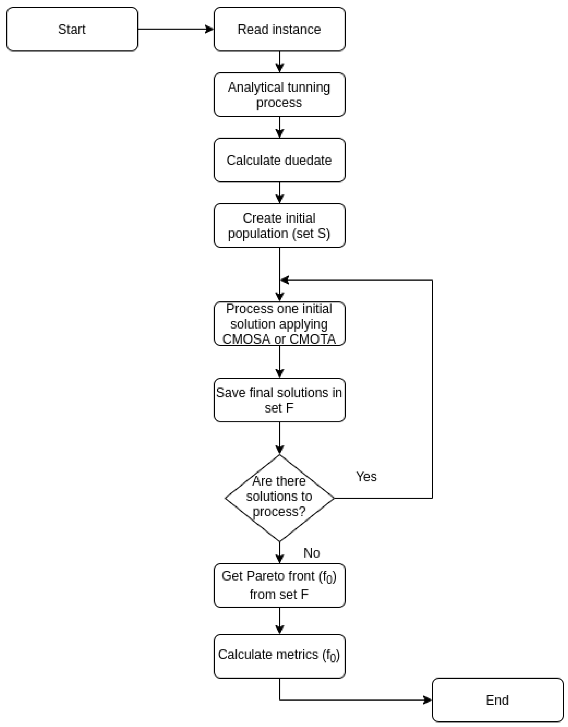
Figure 1 shows the main module for each of the two proposed algorithms CMOSA and CMOTA, which may be considered the main processes in any high-level language.

In this main module, the instance to be solved is read, then the tuning process is performed. The due date is calculated, which is an essential element for calculating the tardiness. The set of initial solutions (S) is generated randomly, as follows. First, a collection of feasible operations are determined, then one of them is randomly selected and added to the solution until all the job operations are added.

Once the set of initial solutions has been generated, an algorithm (CMOSA or CMOTA) is applied to improve each initial solution, and the generated solution is stored in a set of final solutions (F). To obtain the set of non-dominated solutions, also called the zero front ($f_0$) from the set of final solutions, we applied the fast non-dominated Sorting algorithm [29]. To know the quality of the non-dominated set obtained, the MID, Spacing, HV, Spread, IGD, and Coverage metrics are calculated. To perform the calculation of the spread and IGD, the true Pareto front ($P{F}_{true}$) is needed. However, for the instances used in this paper, the $P{F}_{true}$ has not been published for all the instances. For this reason, the calculation was made using an approximate Pareto front ($P{F}_{approx}$), which we obtained from the union of the fronts calculated with previous executions of the two algorithms presented here (CMOSA and CMOTA).

6.1. Computational Experimentation

A set of 70 instances of different authors was used to evaluate the performance of the algorithms, including: (1) FT06, FT10, and FT20 proposed by [40]; (2) ORB01 to ORB10 proposed by [41]; (3) LA01 to LA40 proposed by [42]; (4) ABZ5, ABZ6, ABZ7, ABZ8, and ABZ9 proposed by [43]; (5) YN1, YN2, YN3, and YN4 proposed by [44], and (6) TA01, TA11, TA21, TA31, TA41, TA51, TA61, and TA71 proposed by [30].

As already explained, to perform the analytical tuning, some previous executions of the algorithm are necessary. The parameters used for those previous executions are shown in

Table 2. Tuning parameters for CMOSA/CMOTA.

Number of Executions	Initial Temperature	Final Temperature	Alpha	${\mathit{L}}_{\mathit{k}}$
50	100	0.1	0.98	100

, and the parameters used in the final experimentation for each instance are shown in

Table 3. General parameters for CMOSA/CMOTA.

Number of Executions	Initial Solutions	Alpha	Stagnant Number
30	30	0.98	10

.

The execution of the algorithm was carried out on one of the terminals of the Ehecatl cluster at the TecNM/IT Ciudad Madero, which has the following characteristics: Intel® Xeon® processor at 2.30 GHz, Memory: 64 GB (4 × 16 GB) ddr4-2133, Linux operating system CentOS, and C language was used for the implementation. We developed CMOSA (https://github.com/DrJuanFraustoSolis/CMOSA-JSSP.git) and CMOTA (https://github.com/DrJuanFraustoSolis/CMOTA-JSSP.git) and we tested the software and using three data sets reported in the paper and taken from the literature.

In the first experiment, the algorithms CMOSA and CMOTA were compared with AMOSA algorithm using the 70 described instances and six performance metrics. In a second experiment, we compared CMOSA and CMOTA with the IMOEA/D algorithm, with the 58 instances used by Zhao [14]. In the second experiment, we used the same MID metric of this publication. The third experiment was based on the 15 instances reported in [8], where the results of the next MOJSSP algorithms are published: SPEA, CMOEA, MOPSO, and MOMARLA. In this publication the authors used two objective functions and two metrics (HV and Coverage); they determined that the best algorithm is MOMARLA followed by MOPSO. We executed CMOSA and CMOTA for the instances of this dataset and we compared our results using the HV metric with those published in [8]. However, a comparison using the coverage metric was impossible because the Pareto fronts of these methods have not been reported [8]. In our case, we show in Appendix A the fronts of non-dominated solutions obtained with 70 instances.

6.2. Results

The average values of 30 runs, for the six metrics obtained by CMOSA and CMOTA for the complete data set of 70 instances are shown in

Table 4. Results obtained by the metrics for 70 instances.

Metric	CMOSA	CMOTA	Significant Difference CMOSA-CMOTA
MID	30,680.19 *	31,233.15	Yes
SPACING	28,445.62	28,183.17 *	No
SPREAD	24,969.31	23,401.88 *	No
HV	0.42 *	0.42 *	No
IGD	1666.25 *	1870.94	Yes

* Best result

and

Table 5. Results obtained by the coverage metric.

Coverage (CMOSA, CMOTA)	Coverage (CMOTA, CMOSA)
0.854 *	0.063

* Best result

. We observed that CMOSA obtained the best values for MID and IGD metrics. For Spacing and Spread, CMOTA obtained the best results. For the HV metric, both algorithms achieved the same result (0.42). We observed in Table 5 that CMOSA obtained the best coverage result.

A two-tailed Wilcoxon test was performed with a significance level of 5% (last column in Table 4) and this shows that there are no significant differences between the CMOSA and CMOTA except in MID and IGD metrics.

Table 6. Comparison among CMOSA with AMOSA.

Metric	CMOSA	AMOSA [17]	Significant Difference CMOSA-AMOSA
MID	30,680.19 *	32,138.19	Yes
SPACING	28,445.62 *	30,129.36	Yes
SPREAD	24,969.31 *	26,625.04	No
HV	0.42 *	0.37	No
IGD	1666.25 *	2209.96	Yes

* Best result

shows the comparison of CMOSA and AMOSA. We observed that CMOSA obtains the best performance in all the metrics evaluated. In addition, the Wilcoxon test indicates that there are significant differences in most of them; thus, CMOSA overtakes AMOSA. We compared CMOTA and AMOSA in

Table 7. Comparison among CMOTA with AMOSA.

Metric	CMOTA	AMOSA [17]	Significant Difference CMOTA-AMOSA
MID	31,233.15 *	32,138.19	No
SPACING	28,183.17 *	30,129.36	Yes
SPREAD	23,401.88 *	26,625.04	No
HV	0.42 *	0.37	No
IGD	1870.94 *	2209.96	Yes

* Best result

. In this case, CMOTA also obtains the best average results in all the metrics; however, according to the Wilcoxon test, there are significant differences in only two metrics.

We compare in

Table 8. CMOSA, CMOTA, and IMOEA/D results obtained using MID metric.

CMOSA	CMOTA	IMOEA/D [14]	Significant Difference CMOSA-IMOEA/D	Significant Difference CMOTA-IMOEA/D
15,729.65 *	16,567.07	18,727.04	Yes	Yes

* Best result

the CMOSA and CMOTA with the IMOEA/D algorithm using the 58 common instances published in [14] where the MID metric was measured. This table shows the MID average value of this metric for the non-dominated set of solutions of CMOSA and CMOTA. The results showed that CMOSA and CMOTA obtain better performances than IMOEA/D. We notice that both algorithms, CMOSA and CMOTA, achieved smaller MID values than IMOEA/D, which indicates that the Pareto fronts of our algorithms are closer to the reference point (0,0,0). The Wilcoxon test confirms that CMOSA and CMOTA surpassed the IMOEA/D.

The results of CMOSA and CMOTA were compared with the SPEA, CMOEA, MOPSO, and MOMARLA algorithms [8]. In the last reference, only two objective functions were reported, the makespan and total tardiness. The experimentation was carried out with 15 instances and the average HV values were calculated to perform the analysis of the results, which are shown in

Table 9. Comparison among SPEA, CMOEA, MOPSO, CMOSA, CMOTA, and MOMARLA using HV.

	Instance	SPEA [8]	CMOEA [8]	MOPSO [8]	MOMARLA [8]	CMOSA	CMOTA
1	FT06	0.07	0.07	0.50	0.65	0.64	0.75 *
2	FT10	0.17	0.26	0.87	0.96	0.71	0.69
3	FT20	0.20	0.20	0.21	0.25	0.57 *	0.77 *
4	ABZ5	0.34	0.33	0.36	0.40	0.85 *	0.56 *
5	ABZ6	0.22	0.36	0.31	0.42	0.60 *	0.81 *
6	ABZ7	0.51	0.45	1.00	1.00	0.79	0.51
7	ABZ8	0.88	0.36	0.99	0.99	0.69	0.66
8	LA26	0.33	0.39	0.47	0.47	0.91 *	0.70 *
9	LA27	0.58	0.56	0.41	0.60	0.71 *	0.93 *
10	LA28	0.48	0.42	0.48	0.54	0.92 *	0.44
11	ORB01	0.62	0.74	0.59	0.80	0.87 *	0.63
12	ORB02	0.20	0.04	0.30	0.53	0.88 *	0.77 *
13	ORB03	0.69	0.31	0.85	0.86	0.76	0.80
14	ORB04	0.63	0.28	0.52	0.79	0.76	0.81 *
15	ORB05	0.00	0.023	0.22	0.90	0.74	0.32
	Mean HV	0.39	0.32	0.54	0.68	0.76 *	0.68

* Best result.

. We notice that MOMARLA surpassed SPEA, CMOEA, and MOPSO. We can observe that CMOSA obtained a better performance than MOMARLA and the other algorithms. Comparing CMOTA and MOMARLA, we notice that both algorithms obtained the same HV average results.

6.3. CMOSA-CMOTA Complexity and Run Time Results

In this section, we present the complexity of the algorithms analyzed in this paper. The algorithms’ complexity is presented in

Table 10. Complexity of the algorithms.

AMOSA	IMOEA/D	SPEA	MOPSO	MOMARLA	CMOSA	CMOTA
$O\left(n{\mathsf{\Gamma }}^2\right)$	$O\left(M\mathsf{\Gamma }T\right)$	$O\left(M\mathsf{\Gamma }\right)$	$O\left(M{\mathsf{\Gamma }}^2\right)$	$O\left(Mnp\right)$	$O\left(Mnp\right)$	$O\left(Mnp\right)$

, and it was obtained directly when it was explicitly published or determined from the algorithms’ pseudocodes. In this table, M is the number of objectives, $\mathsf{\Gamma }$ is the population size, T is the neighborhood size, n is the number of iterations (temperatures for AMOSA, CMOSA, and CMOTA), and p is the problem size. The latter is equal to $jm$ where j and m are the number of jobs and machines, respectively. Because the algorithms with the best quality metrics are CMOSA, CMOTA MOMARLA, and MOPSO, their complexity is compared in this section.

It is well known that the complexity of classical SA is $O\left(p^{2}logp\right)$ [45]. However, we notice from Table 10 that CMOSA, and CMOTA have a different complexity even though they are based on SA. This is because these new algorithms applied a different chaotic perturbation and another local search (see Algorithms 2 and 6 in lines 10–20).

The temporal function of MOMARLA, CMOSA, and CMOTA belong to $O\left(Mnp\right)$. For MOMARLA, n is the number of iterations, a variable used at the beginning of this algorithm. On the other hand, for CMOSA and CMOTA, n is the number of temperatures used in the algorithm, also at its beginning; in any case, the difference will be only a constant.

We note that AMOSA and MOPSO have a similar complexity class expression, that is $O\left(n{\mathsf{\Gamma }}^2\right)$ and $O\left(M{\mathsf{\Gamma }}^2\right)$ respectively. However, MOPSO overtakes AMOSA because M is in general lower than n. We observe that CMOSA, CMOTA and MOMARLA belong to $O\left(Mnp\right)$ class complexity, while MOPSO belongs to $O\left(M{\mathsf{\Gamma }}^2\right)$ [46]. Thus, the relation between them is $np/{\mathsf{\Gamma }}^2$ which in general is lower than one. Thus CMOSA, CMOTA and MOMARLA have a lower complexity than MOPSO. Moreover, CMOSA, CMOTA, and MOMARLA have better HV metric quality as is shown in Table 9.

In the next paragraph, we present a comparative analysis of the execution time of the algorithms implemented in this paper.

In

Table 11. Runtimes for CMOSA, CMOTA and AMOSA.

Algorithm	CMOSA	CMOTA	AMOSA [17]
Data set of 70 instances
Average execution time	495.22	229.42 *	505.84
% time saved vs AMOSA	2.1	55 *	0
Data set of 58 instances
Average execution time	111.68	41.97 *	139.39
% time saved vs AMOSA	19.87	69.89 *	0
Data set of 15 instances
Average execution time	81.24	75.24 *	141.25
% time saved vs AMOSA	42.48	46.73 *	0

* Best result

we show the execution time, expressed in seconds, for the three algorithms (CMOSA, CMOTA, and AMOSA) implemented in this paper for three data sets (70, 58, and 15 instances). In all these cases, we emphasize that the AMOSA algorithm was the base to design the other two algorithms. In fact, all of them have the same structure except that CMOSA and CMOTA apply chaotic perturbations when they detect a possible stagnation. Thus, all of them have similar complexity measures for the worst-case. Table 11 shows the percentage of time saved by these two algorithms concerning AMOSA. For these datasets, we measured that AMOSA saved 2.1, 19.87, and 42.48 percent of the AMOSA run time; on the other hand, these figures of CMOTA versus AMOSA are 55, 68.89, and 46.73 percent. Thus, both of our proposed algorithms CMOSA and CMOTA are significantly more efficient than AMOSA. Unfortunately, we do not have the tools to compare these algorithms versus the other algorithms’ execution time in Table 1. Nevertheless, we made the quality comparisons by using the metrics previously published.

7. Conclusions

This paper presents two multi-objective algorithms for JSSP, named CMOSA and CMOTA, with three objectives and six metrics. The objective functions for these algorithms are makespan, total tardiness, and total flow time. Regarding the results from the comparison of CMOSA and CMOTA with AMOSA, we observe that both algorithms obtained a well-distributed Pareto front, closest to the origin, and closest to the approximate Pareto front as was indicated by Spacing, MID, and IGD metrics, respectively. Thus, using these five metrics, we found that CMOSA and CMOTA surpassed the AMOSA algorithm. Regarding the volume covered by the front calculated by the HV metric, it was observed that both algorithms, CMOSA and CMOTA, have the same performance; however, CMOSA has a higher convergence than CMOTA. In addition, the proposed algorithms surpass IMOEA/D when MID metric was used. Moreover, we use the HV to compare the proposed algorithms with SPEA, CMOEA, MOPSO, and MOMARLA. We found that CMOSA outperforms these algorithms, followed by CMOTA, MOMARLA, and MOPSO.

We observe that CMOSA and CMOTA have similar complexity as the best algorithms in the literature. In addition, we show that CMOSA and CMOTA surpass AMOSA when we compare them using execution time for three data sets. We found CMOTA is, on average, 50 percent faster than AMOSA and CMOSA. Finally, we conclude that CMOSA and CMOTA have similar temporal complexity than the best literature algorithms, and the quality metrics show that the proposed algorithms outperform them.

References

1. Coello, C.; Cruz, N. Solving Multiobjective Optimization Problems Using an Artificial Immune System. Genet. Program. Evolvable Mach. 2005, 6, 163–190. [Google Scholar] [CrossRef]
2. Garey, M.R.; Johnson, D.S.; Sethi, R. PageRank: The complexity of flowshop and jobshop scheduling. Math. Oper. Res. 1976, 1, 117–129. [Google Scholar] [CrossRef]
3. Ojstersek, R.; Brezocnik, M.; Buchmeister, B. Multi-objective optimization of production scheduling with evolutionary computation: A review. Int. J. Ind. Eng. Comput. 2020, 11, 359–376. [Google Scholar] [CrossRef]
4. Pinedo, M. Scheduling: Theory, Algorithms, and Systems; Springer-Verlag: New York, NY, USA, 2008. [Google Scholar]
5. Kirkpatrick, S.; Gelatt, C.D.; Vecchi, M.P. Optimization by simulated annealing. Am. Assoc. Adv. Sci. 1983, 220, 671–680. [Google Scholar] [CrossRef] [PubMed]
6. Dueck, G.; Scheuer, T. Threshold Accepting: A General Purpose Algorithm Appearing Superior to Simulated Annealing. J. Comput. Phys. 1990, 90, 161–175. [Google Scholar] [CrossRef]
7. Scaria, A.; George, K.; Sebastian, J. An artificial bee colony approach for multi-objective job shop scheduling. Procedia Technol. 2016, 25, 1030–1037. [Google Scholar] [CrossRef] [Green Version]
8. Méndez-Hernández, B.; Rodriguez Bazan, E.D.; Martinez, Y.; Libin, P.; Nowe, A. A Multi-Objective Reinforcement Learning Algorithm for JSSP. In Proceedings of the 28th International Conference on Artificial Neural Networks, Munich, Germany, 17–19 September 2019; pp. 567–584. [Google Scholar] [CrossRef]
9. López, A.; Coello, C. Study of Preference Relations in Many-Objective Optimization. In Proceedings of the Genetic and Evolutionary Computation Conference (GECCO’ 2009), Montreal, QC, Canada, 8–12 July 2009; pp. 611–618. [Google Scholar] [CrossRef]
10. Blasco, X.; Herrero, J.; Sanchis, J.; Martínez, M. Decision Making Graphical Tool for Multiobjective Optimization Problems; Springer: Berlin/Heidelberg, Germany, 2007; Volume 4527, pp. 568–577. [Google Scholar] [CrossRef]
11. García-León, A.; Dauzère-Pérès, S.; Mati, Y. An Efficient Pareto Approach for Solving the Multi-Objective Flexible Job-Shop Scheduling Problem with Regular Criteria. Comput. Oper. Res. 2019, 108. [Google Scholar] [CrossRef]
12. Qiu, X.; Lau, H.Y.K. An AIS-based hybrid algorithm for static job shop scheduling problem. J. Intell. Manuf. 2014, 25, 489–503. [Google Scholar] [CrossRef] [Green Version]
13. Kachitvichyanukul, V.; Sitthitham, S. A two-stage genetic algorithm for multi-objective job shop scheduling problems. J. Intell. Manuf. 2011, 22, 355–365. [Google Scholar] [CrossRef]
14. Zhao, F.; Chen, Z.; Wang, J.; Zhang, C. An improved MOEA/D for multi-objective job shop scheduling problem. Int. J. Comput. Integr. Manuf. 2016, 30, 616–640. [Google Scholar] [CrossRef]
15. González, M.; Oddi, A.; Rasconi, R. Multi-objective optimization in a job shop with energy costs through hybrid evolutionary techniques. In Proceedings of the Twenty-Seventh International Conference on Automated Planning and Scheduling, Pittsburgh, PA, USA, 18–23 June 2017; pp. 140–148. [Google Scholar]
16. Serafini, P. Simulated Annealing for Multi Objective Optimization Problems. In Proceedings of the Tenth International Conference on Multiple Criteria Decision Making, Taipei, Taiwan, 19–24 July 1992. [Google Scholar]
17. Bandyopadhyay, S.; Saha, S.; Maulik, U.; Deb, K. A Simulated Annealing-Based Multiobjective Optimization Algorithm: AMOSA. Evol. Comput. IEEE Trans. 2008, 12, 269–283. [Google Scholar] [CrossRef] [Green Version]
18. Liu, Y.; Dong, H.; Lohse, N.; Petrovic, S.; Gindy, N. An Investigation into Minimising Total Energy Consumption and Total Weighted Tardiness in Job Shops. J. Clean. Prod. 2013, 65, 87–96. [Google Scholar] [CrossRef]
19. Zitzler, E.; Thiele, L. Multiobjective Evolutionary Algorithms: A Comparative Case Study and the Strength Pareto Approach. IEEE Trans. Evol. Comput. 2000, 3, 257–271. [Google Scholar] [CrossRef] [Green Version]
20. Wisittipanich, W.; Kachitvichyanukul, V. An Efficient PSO Algorithm for Finding Pareto-Frontier in Multi-Objective Job Shop Scheduling Problems. Ind. Eng. Manag. Syst. 2013, 12, 151–160. [Google Scholar] [CrossRef]
21. Lei, D.; Wu, Z. Crowding-measure-based multiobjective evolutionary algorithm for job shop scheduling. Int. J. Adv. Manuf. Technol. 2006, 30, 112–117. [Google Scholar] [CrossRef]
22. Kurdi, M. An Improved Island Model Memetic Algorithm with a New Cooperation Phase for Multi-Objective Job Shop Scheduling Problem. Comput. Ind. Eng. 2017, 111, 183–201. [Google Scholar] [CrossRef]
23. Méndez-Hernández, B.; Ortega-Sánchez, L.; Rodriguez Bazan, E.D.; Martinez, Y.; Fonseca-Reyna, Y. Bi-objective Approach Based in Reinforcement Learning to Job Shop Scheduling. Revista Cubana de Ciencias Informáticas 2017, 11, 175–188. [Google Scholar]
24. Aarts, E.H.L.; van Laarhoven, P.J.M.; Lenstra, J.K.; Ulder, N.L.J. A Computational Study of Local Search Algorithms for Job Shop Scheduling. INFORMS J. Comput. 1994, 6, 118–125. [Google Scholar] [CrossRef]
25. Ponnambalam, S.G.; Ramkumar, V.; Jawahar, N. A multiobjective genetic algorithm for job shop scheduling. Prod. Plan. Control 2001, 12, 764–774. [Google Scholar] [CrossRef]
26. Suresh, R.K.; Mohanasundaram, M. Pareto archived simulated annealing for job shop scheduling with multiple objectives. Int. J. Adv. Manuf. Technol. 2006, 29, 184–196. [Google Scholar] [CrossRef]
27. Zitzler, E.; Deb, K.; Thiele, L. Comparison of Multiobjective Evolutionary Algorithms: Empirical Results. Evol. Comput. 2000, 8, 173–195. [Google Scholar] [CrossRef] [PubMed] [Green Version]
28. Karimi, N.; Zandieh, M.; Karamooz, H. Bi-objective group scheduling in hybrid flexible flowshop: A multi-phase approach. Expert Syst. Appl. 2010, 37, 4024–4032. [Google Scholar] [CrossRef]
29. Deb, K.; Agrawal, S.; Pratap, A.; Meyarivan, T. Agrawal, S.; Pratap, A.; Meyarivan, T. A fast elitist non-dominated sorting genetic algorithm for multi-objective optimization: NSGA-II. In International Conference on Parallel Problem Solving from Nature; Spring: Berlin/Heidelberg, Germany, 2000; Volume 1917. [Google Scholar]
30. Taillard, E. Benchmarks for basic scheduling problems. Eur. J. Oper. Res. 1993, 64, 278–285. [Google Scholar] [CrossRef]
31. Deb, K. Multiobjective Optimization Using Evolutionary Algorithms; Wiley: New York, NY, USA, 2001. [Google Scholar]
32. Schott., J.R. Fault Tolerant Design Using Single and Multicriteria Genetic Algorithm Optimization. Master’s Thesis, Department of Aeronautics and Astronautics, Massachusetts Institute of Technology, Cambridge, MA, USA, 1995.
33. Veldhuizen, D.A.V. Multiobjective Evolutionary Algorithms: Classifications, Analyses, and New Innovations. Ph.D. Thesis, Air Force Institute of Technology, Wright-Patterson AFB, Dayton, OH, USA, 1999. [Google Scholar]
34. Sawaragi, Y.; Nakagama, H.; Tanino, T. Theory of Multi-Objective Optimization; Springer: Boston, MA, USA, 1985. [Google Scholar]
35. Bakuli, D.L. A Survey of Multi-Objective Scheduling Techniques Applied to the Job Shop Problem (JSP). In Applications of Management Science: In Productivity, Finance, and Operations; Emerald Group Publishing Limited: Bingley, UK, 2015; pp. 51–62. [Google Scholar]
36. Baker, K.R. Sequencing rules and due-date assignments in job shop. Manag. Sci. 1984, 30, 1093–1104. [Google Scholar] [CrossRef]
37. Sanvicente, S.H.; Frausto, J. A method to establish the cooling scheme in simulated annealing like algorithms. In International Conference on Computational Science and Its Applications; Springer: Berlin/Heidelberg, Germany, 2004; pp. 755–763. [Google Scholar]
38. Solís, J.F.; Sánchez, H.S.; Valenzuela, F.I. ANDYMARK: An analytical method to establish dynamically the length of the Markov chain in simulated annealing for the satisfiability problem. Lect. Notes Comput. Sci. 2006, 4247, 269–276. [Google Scholar]
39. May, R. Simple Mathematical Models With Very Complicated Dynamics. Nature 1976, 26, 457. [Google Scholar] [CrossRef] [PubMed]
40. Fisher, H.; Thompson, G.L. Probabilistic learning combinations of local job-shop scheduling rules. Ind. Sched. 1963, 1, 225–251. [Google Scholar]
41. Applegate, D.; Cook, W. A computational study of the job-shop scheduling problem. ORSA J. Comput. 1991, 3, 149–156. [Google Scholar] [CrossRef]
42. Lawrence, S. Resource Constrained Project Scheduling: An Experimental Investigation of Heuristic Scheduling Techniques (Supplement); Graduate School of Industrial Administration, Carnegie-Mellon University: Pittsburgh, PA, USA, 1984. [Google Scholar]
43. Adams, J.; Balas, E.; Zawack, D. The shifting bottleneck procedure for job shop scheduling. Manag. Sci. 1988, 34, 391–401. [Google Scholar] [CrossRef]
44. Yamada, T.; Nakano, R. A genetic algorithm applicable to large-scale job-shop problems. In Proceedings of the Second International Conference on Parallel Problem Solving from Nature, Brussels, Belgium, 28–30 September1992; pp. 281–290. [Google Scholar]
45. Hansen, P.B. Simulated Annealing. In Electrical Engineering and Computer Science-Technical Reports; School of Computer and Information Science, Syracuse University: Syracuse, NY, USA, 1992. [Google Scholar]
46. Tripathi, P.K.; Bandyopadhyay, S.; Pal, S.K. Multi-Objective Particle Swarm Optimization with time variant inertia and acceleration coefficients. Inf. Sci. 2007, 177, 5033–5049. [Google Scholar] [CrossRef] [Green Version]
Figure 1. Main module for CMOSA and CMOTA.
Mca 26 00008 g001