A Non-Standard Finite Difference Scheme for Magneto-Hydro Dynamics Boundary Layer Flows of an Incompressible Fluid Past a Flat Plate

Abstract

This paper deals with a non-standard implicit finite difference scheme that is defined on a quasi-uniform mesh for approximate solutions of the Magneto-Hydro Dynamics (MHD) boundary layer flow of an incompressible fluid past a flat plate for a wide range of the magnetic parameter. The proposed approach allows imposing the given boundary conditions at infinity exactly. We show how to improve the obtained numerical results via a mesh refinement and a Richardson extrapolation. The obtained numerical results are favourably compared with those available in the literature.

1. Introduction

The simplest example of the application of the boundary layer theory is related to the celebrated Blasius [1] problem. This problem describes the flow around a very thin flat plate.

The first goal of this paper is to numerically solve, with great accuracy, the Magneto-Hydro Dynamics (MHD) boundary layer equation that governs the flow of an incompressible fluid past a flat plate by an implicit non-standard finite difference scheme that is defined on a quasi-uniform mesh that allows imposing the given boundary conditions exactly.

Numerical methods for problems, like the one considered in this paper, can be classified according to the numerical treatment of the boundary condition imposed at infinity. The oldest and simplest treatment is to replace infinity with a suitable finite value, the so-called truncated boundary. However, being the simplest approach, this has revealed, within the decades, some drawbacks that suggest not to apply it, especially if we have to face a given problem without any clue on its solution behaviour. Several other treatments have been proposed in the literature to overcome the shortcomings of the truncated boundary approach. In this research area, some treatments are worthy of consideration: the formulation of so-called asymptotic boundary conditions by de Hoog and Weiss [2], Lentini and Keller [3], and Markowich [4,5]; the reformulation of the given problem in a bounded domain, as first studied by de Hoog and Weiss and more recently developed by Kitzhofer et al. [6]; the free boundary formulation that was proposed by Fazio [7], where the unknown free boundary can be identified with a truncated boundary; the treatment on the original domain via pseudo-spectral collocation methods, see the book by Boyd [8] or the review by Shen and Wang [9] for more details on this topic; and, finally, a non-standard finite difference scheme on a quasi-uniform grid that is defined on the original domain by Fazio and Jannelli [10]. The proposed non-standard finite difference scheme has been successively modified by Fazio and Jannelli [11] and used in [12,13]. Moreover, this method has been applied to the numerical solution of the perpetual American put option problem of financial markets, see Fazio [14].

The key advantage of the presented approach is that the given BVP is solved on a semi-infinite interval by introducing a stencil that is constructed in such a way that the boundary conditions at infinity are exactly assigned. In this way, the whole infinite domain is taken into account in the mapping where the grid-points are located at the mid-point of each sub-interval, and then the difficulty that is caused by numerical treatment of the last infinite sub-interval is avoided.

Finally, via a mesh refinement, by using Richardson’s extrapolation, we improve the accuracy of the obtained numerical results, showing that they are in excellent agreement with the solutions found in the literature. This study concludes by comparing the current numerical results with those that are given by the integral approximation method (ITM) and the non-integral technique (NIT) used by Singh and Chandarki [15].

2. Model Problem

We consider a steady two-dimensional flow of a viscous fluid on a flat plate in the presence of a given transverse magnetic field with small electric conductivity and a large transverse magnetic field. When introducing appropriate similarity variables, the governing equations can be reduced to the following boundary value problem (BVP) [15]

$$\begin{array}{cc}\hfill & {\displaystyle \frac{d^{3}u}{d{x}^3}}+u{\displaystyle \frac{d^{2}u}{d{x}^2}}+\beta \left(1-{\displaystyle \frac{du}{dx}}\right)=0\\ \hfill & \\ & u\left(0\right)={\displaystyle \frac{du}{dx}}\left(0\right)=0,{\displaystyle \frac{du}{dx}}(\infty )=1,\end{array}$$

(1)

where $\beta$ is the magnetic parameter. Let us notice that, for $\beta =0$, the BVP (1) reduces to the celebrated Blasius problem [1]. For a general class of problems, including (1), Brighi [16] obtained results on the existence, uniqueness, and boundedness of solutions.

3. The Finite Difference Scheme

Without a loss of generality, we consider the class of BVPs

$$\begin{array}{ccc}& & {\displaystyle \frac{d\mathbf{u}}{dx}}=\mathbf{f}\left(x,\mathbf{u}\right),x\in [0,\infty ),\hfill \\ \hfill \\ & & \mathbf{g}\left(\mathbf{u}\left(0\right),\mathbf{u}(\infty )\right)=\mathbf{0},\hfill \end{array}$$

(2)

where $\mathbf{u}\left(x\right)$ is a $d—$dimensional vector with ${}^{\ell }u\left(x\right)$ for $\ell =1,\cdots ,d$ as components, $\mathbf{f}:[0,\infty )\times \mathrm{I}{\mathrm{R}}^d\to \mathrm{I}{\mathrm{R}}^d$, and $\mathbf{g}:\mathrm{I}{\mathrm{R}}^d\times \mathrm{I}{\mathrm{R}}^d\to \mathrm{I}{\mathrm{R}}^d$. Here, and in the following, we use Lambert’s notation for the vector components [17] (pp. 1–5).

In order to solve the problem (2) on the original domain, we first discuss quasi-uniform grids maps from a reference finite domain and then introduce, on the original domain, a non-standard finite difference scheme that allows for us to impose the given boundary conditions exactly. Let us consider the smooth strict monotone quasi-uniform maps $x=x\left(\xi \right)$, the so-called grid generating functions, see Boyd [8] (pp. 325–326) or Canuto et al. [18] (p. 96),

$$x=-c·ln(1-\xi ),$$

(3)

and

$$x=c\frac{\xi }{1-\xi },$$

(4)

where $\xi \in \left[0,1\right]$, $x\in \left[0,\infty \right]$, and $c>0$ is a control parameter. Accordingly, a family of uniform grids ${\xi }_n=n/N$ defined on interval $[0,1]$ generates one parameter family of quasi-uniform grids $x_n=x\left({\xi }_n\right)$ on the interval $[0,\infty ]$. The two maps (3) and (4) are referred to as logarithmic and algebraic maps, respectively. As far as the authors’ knowledge is concerned, van de Vooren and Dijkstra [19] were the first to use these kinds of maps. We notice that more than half of the intervals are in the domain with a length approximately equal to c and $x_{N-1}=clnN$ for (3), while $x_{N-1}\approx cN$ for (4). For both maps, the equivalent mesh in x is nonuniform, with the most rapid variation occurring with $c\ll x$. The logarithmic map (3) gives slightly better resolution near $x=0$ than the algebraic map (4), while the algebraic map gives much better resolution than the logarithmic map as $x\to \infty$. In fact, it is easily verified that

$$-c·ln(1-\xi )<c\frac{\xi }{1-\xi },$$

for all $\xi$, but $\xi =0$.

The problem under consideration can be discretized by introducing a uniform grid ${\xi }_n$ of $N+1$ nodes in $\left[0,1\right]$ with ${\xi }_0=0$ and ${\xi }_{n+1}={\xi }_n+h$ with $h=1/N$, so that $x_n$ is a quasi-uniform grid in $\left[0,\infty \right]$. The last interval in (3) and (4), namely $\left[x_{N-1},x_N\right]$, is infinite, but the point $x_{N-1/2}$ is finite, because the non integer nodes are defined by

$$x_{n+\alpha }=x\left(\xi =\frac{n+\alpha }{N}\right),$$

with $n\in \{0,1,\dots ,N-1\}$ and $0<\alpha <1$. These maps allow for us to describe the infinite domain by a finite number of intervals. The last node of such grid is placed on infinity, so right boundary conditions are correctly taken into account.

We approximate the values of the scalar variable $u\left(x\right)$ and its derivative at mid-points of the grid $x_{n+1/2}$, for $n=0,\cdots ,N-1$, while using non-standard difference discretizations

$$\begin{array}{ccc}\hfill u_{n+1/2}& \approx & \frac{x_{n+3/4}-x_{n+1/2}}{x_{n+3/4}-x_{n+1/4}}{u}_n+\frac{x_{n+1/2}-x_{n+1/4}}{x_{n+3/4}-x_{n+1/4}}{u}_{n+1},\hfill \\ \hfill \\ \hfill {\left.\frac{du}{dx}\right|}_{n+1/2}& \approx & \frac{u_{n+1}-u_n}{2\left(x_{n+3/4}-x_{n+1/4}\right)}.\hfill \end{array}$$

(5)

We emphasize that the key advantage of our non-standard finite difference formulation is to overcome the difficulty of the numerical treatment of the boundary conditions at infinity. In fact, the formulae (5) use the value $u_N=u(\infty )$, but not $x_N=\infty$ and, then, the boundary conditions at infinity are taken into account in a natural way.

For the class of BVPs (2), a non-standard finite difference scheme on a quasi-uniform grid can be defined using the approximations given by (5) above, and it can be written, as follows

$$\begin{array}{cc}& {\mathbf{U}}_{n+1}-{\mathbf{U}}_n-a_{n+1/2}\mathbf{f}\left(x_{n+1/2},b_{n+1/2}{\mathbf{U}}_{n+1}+c_{n+1/2}{\mathbf{U}}_n\right)=\mathbf{0},\\ & forn=0,1,\dots ,N-1\\ & \mathbf{g}\left({\mathbf{U}}_0,{\mathbf{U}}_N\right)=\mathbf{0},\end{array}$$

(6)

where

$$\begin{array}{ccc}\hfill a_{n+1/2}& =& 2\left(x_{n+3/4}-x_{n+1/4}\right),\hfill \\ \hfill b_{n+1/2}& =& \frac{x_{n+1/2}-x_{n+1/4}}{x_{n+3/4}-x_{n+1/4}},\hfill \\ \hfill c_{n+1/2}& =& \frac{x_{n+3/4}-x_{n+1/2}}{x_{n+3/4}-x_{n+1/4}},\hfill \end{array}$$

(7)

for $n=0,1,\dots ,N-1$. The finite difference formulation (6) has an order of accuracy $O\left(N^{-2}\right)$. It is evident that (6) is a nonlinear system of $d(N+1)$ equations in the $d(N+1)$ unknowns $\mathbf{U}={({\mathbf{U}}_0,{\mathbf{U}}_1,\dots ,{\mathbf{U}}_N)}^T$. For the solution of (6), we can apply the classical Newton’s method along with the simple termination criterion

$${\displaystyle \frac{1}{d(N+1)}\sum _{\ell =1}^d\sum _{n=0}^N|\Delta {}^{\ell }{U}_n|\le \mathrm{TOL}},$$

(8)

where $\Delta {}^{\ell }{U}_n$, for $n=0,1,\dots ,N$ and $\ell =1,2,\dots ,d$, is the difference between two successive iterate components and $\mathrm{TOL}$ is a fixed tolerance.

4. Numerical Results and Comparison

In this Section, we present the numerical results that were obtained by solving the mathematical model (1) using the non-standard finite difference scheme (6) on the quasi-uniform grid that was defined by the logarithmic map (3) with control parameter $c=2$. The control parameter c defines the grid points distribution in the original physical infinite domain and it is chosen in such a way that $[x_0,x_{N-1}]$ is not too large, being $x_N\to \infty$. The chosen value $c=2$ leads to obtaining a finer grid points distribution close to $x=0$ and then a better resolution where the solution has a transient behavior, with an increasing spatial resolution going toward infinity.

Now, let us rewrite the model (1) as a first-order system, as follows

$$\begin{array}{ccc}& & \frac{d{}^{1}u}{dx}={}^{2}u,\hfill \\ & & \frac{d{}^{2}u}{dx}={}^{3}u,x\in (0,\infty )\hfill \\ & & \frac{d{}^{3}u}{dx}=-{}^{1}u{}^{3}u-\beta (1-{}^{2}u),\hfill \end{array}$$

(9)

with

$$\begin{array}{c}\hfill \begin{array}{c}{}^{1}u\left(0\right)={}^{2}u\left(0\right)=0,{}^{2}u(\infty )=1,\hfill \end{array}\end{array}$$

or, in an equivalent form,

$$\begin{array}{ccc}& & \mathbf{u}={({}^{1}u,{}^{2}u,,{}^{3}u)}^T,\hfill \\ & & \mathbf{f}(x,\mathbf{u})={\left({}^{2}u,{}^{3}u,-{}^{1}u{}^{3}u-\beta (1-{}^{2}u)\right)}^T,\hfill \\ & & \mathbf{g}(\mathbf{u}\left(0\right),\mathbf{u}(\infty ))={({}^{1}u\left(0\right),{}^{2}u\left(0\right),{}^{2}u(\infty )-1)}^T,\hfill \end{array}$$

where $\mathbf{u}\left(x\right)$ is a three-dimensional vector with components ${}^{\ell }u\left(x\right)$ for $\ell =1,2,3$, and $\mathbf{f}:[0,\infty )\times \mathrm{I}{\mathrm{R}}^d\to \mathrm{I}{\mathrm{R}}^d$ and $\mathbf{g}:\mathrm{I}{\mathrm{R}}^d\times \mathrm{I}{\mathrm{R}}^d\to \mathrm{I}{\mathrm{R}}^d$, with $d=3$.

For all tests, we consider the control parameter $c=2$, a fixed tolerance $\mathrm{TOL}={10}^{-8}$, and, as a first guess for Newton’s iteration, the following initial data

$$\begin{array}{ccc}\hfill & & {}^{1}u\left(x\right)=0.5x,{}^{2}u\left(x\right)=1,{}^{3}u\left(x\right)=exp(-x).\hfill \end{array}$$

In

Table 1. Numerical results that are related to ${\displaystyle \frac{d^{2}u}{d{x}^2}}\left(0\right)$ for different values of N.

N	Iter	${\displaystyle \frac{{\mathit{d}}^2\mathit{u}}{{\mathit{dx}}^2}}\left(0\right)$
10	6	$1.1790527$
20	6	$1.1776846$
40	6	$1.1773411$
80	6	$1.1772552$
160	6	$1.1772336$
320	7	$1.1772282$
640	7	$1.1772269$
1280	7	$1.1772261$

, we report the numerical results that were obtained for the missing initial data ${\displaystyle \frac{d^{2}u}{d{x}^2}}$ for increasing points number N and $\beta =1.2$. Here, “iter ”stands for the number of the Newton’s iterations. It is well known that Newton’s method could have a computational cost that is quite high, depending on the initial iterate and the analytic form of the function whose root is being sought. A suitable choice of the initial iterate can contribute to reducing the computational cost. In this context, the chosen initial guess leads to obtain a low iterations number: 6 or 7 iterations, depending on the values of the grid point number.

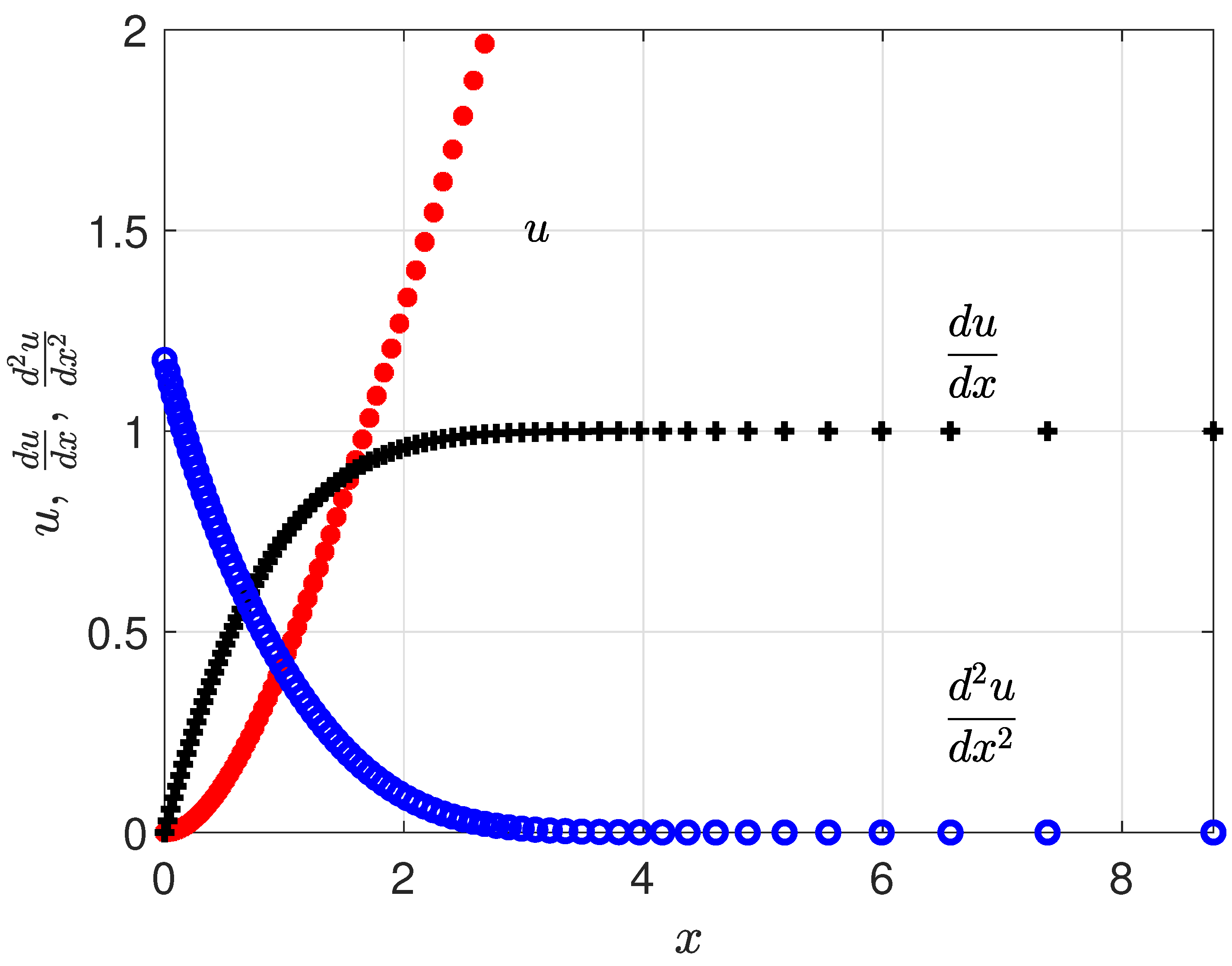
In Figure 1, we show the numerical solution that was obtained for $\beta =1.2$ and $N=80$. The recovered value of the second order derivative of the solution at the origin is ${\displaystyle \frac{d^{2}u}{d{x}^2}}\left(0\right)=1.177255155089504$, obtained in 6 iterations.

Table 2. Numerical results, related to ${\displaystyle \frac{d^{2}u}{d{x}^2}}\left(0\right)$, and comparison with results by [15].

$\mathit{\beta }$	DTM [15]	FD (This Study)	Err Rel
0.0	0.46910	0.4695839	0.0010
0.2	0.66343	0.6389912	0.0382
0.4	0.80009	0.7749739	0.0324
0.6	0.91659	0.8917536	0.0279
0.8	1.01988	0.9956343	0.0244
1.0	1.11362	1.0900815	0.0216
1.2	1.20006	1.1772448	0.0194
1.4	1.28068	1.2585668	0.0176
1.6	1.35652	1.3350710	0.0161
1.8	1.42834	1.4075142	0.0148
2.0	1.49671	1.4764751	0.0137

and

Table 3. Numerical results, related to ${\displaystyle \frac{d^{2}u}{d{x}^2}}\left(0\right)$, and comparison with results by [15].

$\mathit{\beta }$	NIT [15]	FD (This Study)	Err Rel
0.0	0.46920	0.4695839	0.0008
0.2	0.64819	0.6389912	0.0174
0.4	0.78749	0.7749739	0.0162
0.6	0.90562	0.8917536	0.0156
0.8	1.01002	0.9956343	0.0145
1.0	1.10460	1.0900815	0.0133
1.2	1.19170	1.1772448	0.0123
1.4	1.27285	1.2585668	0.0113
1.6	1.34913	1.3350710	0.0105
1.8	1.42132	1.4075142	0.0098
2.0	1.49002	1.4764751	0.0092

list the obtained numerical results for different values of parameter $\beta$, with $\beta =0,0.2,\cdots ,2$ and $N=100$. For the sake of brevity, we have chosen to only report the values of the wall shear stress, which is the second derivative value at the origin. Within the same table, we can compare our results with those that were reported by Singh and Chandarki [15]. The last column, named Err Rel, reports the values of the relative errors, as computed by

$$RelErr=\frac{\left|DTM-FD\right|}{\left|FD\right|}RelErr=\frac{\left|NIT-FD\right|}{\left|FD\right|}$$

where, DTM, NIT, and FD represent the numerical solutions obtained, for different values of $\beta$, by the integral approximation method (ITM) and the non-integral technique (NIT) used by Singh and Chandarki [15], and by the proposed numerical method, respectively. In both cases, the value of the relative errors decrease as the values of $\beta$ increase. Note that the relative errors are all of same the order and, moreover, for $\beta =0$, we obtain the smaller relative error. This is due to the fact that $\beta$ affects the non-linearity of the model under study. The problem with $\beta =0$ corresponding to the Blasius problem and, in this case, the computed missing initial condition ${\displaystyle \frac{d^{2}u}{d{x}^2}}\left(0\right)=0.4695839$ can be compared with the value $0.469599988361$ that wascomputed by Fazio [7] by a free boundary formulation of the Blasius problem.

We apply Richardson’s extrapolation, using several refinements of the computational domain, in order to improve the accuracy of the computed solution. On the computational domain of the problem, we build a quasi-uniform grid with a mesh-points number equal to $N_0$ and proceed with subsequent grid refinements by constructing meshes with grid-point numbers $N_g$ for $g=1,2,\cdots$, where $N_{g+1}=r{N}_g$ with refinement factor $r=2$. On each grid, the numerical solution $U_g$, $g=0,1,\cdots ,G$ is computed using the non-standard finite difference method. We adopt a continuation strategy in order to reduce the calculations; in fact, we use the final solution $U_g$ that was obtained on the grid g as an initial guess for calculating the solution $U_{g+1}$ on the grid $g+1$, where the new grid values are approximated by linear interpolations. We define the level of the Richardson’s extrapolation by the index k and the two numerical solutions related to the grids g and $g+1$ at the extrapolated level k by $U_{g,k}$ and $U_{g+1,k}$. We use the following formula to calculate a more accurate approximation

$$U_{g+1,k+1}=U_{g+1,k}+\frac{U_{g+1,k}-U_{g,k}}{2^{p_k}-1}k=0,1,\cdots ,G-1.$$

(10)

In

Table 4. Extrapolated values at origin $x=0$ for ${\displaystyle \frac{d^{2}u}{d{x}^2}}\left(0\right)$ with $\beta =1$.

${\mathit{N}}_{\mathit{g}}$	${}^3{\mathit{U}}_{\mathit{g},0}$	${}^3{\mathit{U}}_{\mathit{g},1}$	${}^3{\mathit{U}}_{\mathit{g},2}$
100	$1.090081494$	-	-
200	$1.090069055$	$1.090064908$	-
400	$1.090065945$	$1.090064908$	$1.090064908$

, we report the extrapolated values with $N=100,200,400$ grid points for $\beta =1$. The last extrapolated value is ${}^3{U}_{2,2}=1.090064908$ and it can be considered as our benchmark value for ${\displaystyle \frac{d^{2}u}{d{x}^2}}\left(0\right)$. We can conclude that the reported extrapolated value is correct up to 9 decimal places.

5. Concluding Remarks

In this paper, the mathematical model, which describes the MHD boundary layer flow of an incompressible fluid past a flat plate, is solved by the non-standard implicit finite difference method on a quasi-uniform grid for the different magnetic parameters $\beta$. We solved the given BVP on a semi-infinite interval by introducing a stencil that is built in such a way that the boundary conditions at infinity are exactly assigned. Moreover, we improved the accuracy of the numerical results by Richardson’s extrapolation, which allowed for us to find a more accurate solution.

The values of the second-order derivative of the solution at the origin, for different values of parameter $\beta$, are reported in the Table 2 and Table 3. The results are compared with those by Singh and Chandarki [15] in order to verify the accuracy of the proposed method. Moreover, in the case of the Blasius problem, we compare the missing initial condition with the one that was computed by Fazio [7] by a free boundary formulation of the Blasius problem. The computed values are found to be really accurate.