Article

Exponential Perturbative Expansions and Coordinate Transformations

Institut de Matemàtiques i Aplicacions de Castelló (IMAC) and Departament de Matemàtiques, Universitat Jaume I, E-12071 Castellón, Spain
*
Author to whom correspondence should be addressed.
Math. Comput. Appl. 2020, 25(3), 50; https://doi.org/10.3390/mca25030050
Submission received: 3 July 2020 / Revised: 10 August 2020 / Accepted: 11 August 2020 / Published: 13 August 2020

Abstract

:
We propose a unified approach for different exponential perturbation techniques used in the treatment of time-dependent quantum mechanical problems, namely the Magnus expansion, the Floquet–Magnus expansion for periodic systems, the quantum averaging technique, and the Lie–Deprit perturbative algorithms. Even the standard perturbation theory fits in this framework. The approach is based on carrying out an appropriate change of coordinates (or picture) in each case, and it can be formulated for any time-dependent linear system of ordinary differential equations. All of the procedures (except the standard perturbation theory) lead to approximate solutions preserving by construction unitarity when applied to the time-dependent Schrödinger equation.

1. Introduction

Linear differential equations of the form
d U d t = A ( t ) U , U ( 0 ) = I
are ubiquitous in many branches of physics, chemistry and mathematics. Here, U is a real or complex d × d matrix, and A ( t ) is a sufficiently smooth matrix to ensure the existence of solutions. Perhaps the most important example corresponds to the Schrödinger equation for the evolution operator in quantum systems with a time-dependent Hamiltonian H ( t ) , in which case A ( t ) = i H ( t ) / . Particular cases include spin dynamics in magnetic resonance (Nuclear Magnetic Resonance—NMR, Electronic Paramagnetic Resonance—EPR, Dynamic Nuclear Polarization—DNP, etc.) [1,2,3], electron-atom collisions in atomic physics, pressure broadening of rotational spectra in molecular physics, control of chemical reactions with driving induced by laser beams, etc. When the time-dependence of the Hamiltonian is periodic, as occurs, for instance, in periodically driven quantum systems, atomic quantum gases in periodically driven optical lattices, etc. [4,5], the Floquet theorem [6] relates H ( t ) with a constant Hamiltonian. More specifically, it implies that the evolution operator is factorized as U ( t ) = P ( t ) exp ( t F ) , with P ( t ) a periodic time-dependent matrix and F a constant matrix. This theorem has been widely used in problems of solid state physics, in NMR, in the quantum simulation of systems with time-independent Hamiltonians by periodically driven quantum systems, etc. [7]. The Average Hamiltonian Theory is also closely related with this result, and the effective Hamiltonian is an important tool in the description of the system [8,9].
In general, Equation (1) cannot be solved in closed form, and so different approaches have been proposed along the years to obtain approximations, both analytic and numerical. Among the former, we can mention the standard perturbation theory, the average Hamiltonian theory, and the Magnus expansion [5,8,10]. Concerning the second approach, different numerical algorithms have been applied to obtain solutions on specific time intervals [11,12,13].
In this work, we will concentrate on different techniques providing analytic approximations to the solution of (1) that also share some of its most salient qualitative features. In particular, if (1) represents the Schrödinger equation, it is well known that U ( t ) is unitary for all t, and this guarantees that its elements represent probabilities of transition between the different states of the system. However, it happens that not every approximate scheme (either analytic or numerical) renders unitary matrices and, thus, the physical description they provide is unreliable, especially for large integration times.
The Magnus expansion [14] presents the remarkable feature that it allows one to express the solution as the exponential of a series, U ( t ) = exp ( Ω ( t ) ) , so that, even when the series Ω ( t ) = n 1 Ω n ( t ) is truncated, the corresponding approximation is still unitary when applied to the Schrödinger equation. More generally, if (1) is defined in a Lie group G , then it provides an approximate solution also belonging to G . Moreover, it has also been used to construct efficient numerical integration algorithms also preserving this feature [12,15].
When A ( t ) periodically depends on time with period T, the Magnus expansion does not explicitly provide the structure of the solution ensured by the Floquet theorem, i.e., U ( t ) = P ( t ) e t F . with P ( t ) periodic and F a constant matrix. Nevertheless, it can be conveniently generalized to cover also this situation, in such a way that the matrix P ( t ) is expressed as the exponential of a series of periodic terms. The resulting approach (the so-called Floquet–Magnus expansion [10]) has been used during the last years in a variety of physical problems [4,5,7,16].
Very often, the coefficient matrix in (1) is of the form A ( t ) = A 0 + ε A 1 ( t ) , where A 0 is constant, A 1 ( t + T ) = A 1 ( t ) , and ε > 0 is a (small) parameter. In other words, one is dealing with a time-dependent perturbation of a solvable problem defined by A 0 . In that case, several perturbative procedures exist to construct U ( t ) as a power series in ε , either directly (by applying standard perturbation techniques in the interaction picture defined by A 0 ) or taking into account the structure ensured by the Floquet theorem and constructing both matrices P ( t ) and F as power series [9]. Of course, if P ( t ) = exp ( Λ ( t ) ) and Λ ( t ) is also constructed as a power series in ε , then the qualitative properties of the solution are inherited by the approximations (in particular, they are unitary in quantum evolution problems) [17].
An alternative manner of viewing the Floquet theorem is to interpret the matrix P ( t ) , provided that it is invertible, as a time-periodic transformation to a new set of coordinates where the new evolution equation has a constant coefficient matrix F, so that exp ( t F ) is the exact solution in the new coordinates. In the language of Quantum Mechanics, this corresponds to a change of picture. This interpretation leads to the important mathematical notion of a reducible system: according to Lyapunov, the general system (1) is called reducible if there exists a matrix P ( t ) which together with det ( P 1 ( t ) ) is bounded on 0 t < + , such that the system obtained from (1) by applying the linear transformation defined by P ( t ) has constant coefficients [18]. In this sense, if A ( t ) is a periodic matrix, then (1) is reducible by means of a periodic matrix. The situation is not so clear; however, when A ( t ) is quasi-periodic or almost periodic: although several general results exist ensuring reducibility [19,20,21], there are also examples of irreducible systems [22].
In this work, we pursue and generalize this interpretation to show that all of the above mentioned exponential perturbative treatments can be considered as particular instances of a generic change of variables applied to the original differential equation. The idea of making a coordinate change to analyze a problem arises of course in many application settings, ranging from canonical (or symplectic) transformations in classical mechanics (based either on generating functions expressed in terms of mixed, old and new, variables [23], or on the Lie-algebraic setting [24,25]) to changes of picture and unitary transformations in quantum mechanics. What we intend here is to show that several widely used perturbative expansions in quantum mechanics can be indeed derived from the same basic principle using different variations of a unique ansatz based on a generic linear transformations of coordinates. We believe that this interpretation sheds new light into the different expansions and, moreover, allows one to elaborate a unique procedure for analyzing a given problem and compare in an easy way how they behave in practice.
It is important to remark that all the procedures considered here (with the exception of course of the standard perturbation theory) preserve by construction the unitarity of the solution when (1) refers to the Schrödinger equation. More generally, the approximations obtained evolve in the same matrix Lie group as the exact solution of the differential Equation (1).

2. Coordinate Transformations and Linear Systems

To begin with, let us consider the most general situation of a linear differential equation
x ˙ d x d t = A ( t ) x , x ( 0 ) = x 0 C d ,
with A ( t ) a d × d matrix whose entries are integrable functions of t. Notice that U ( t ) in (1) can be considered the fundamental matrix of (2). We analyze a change of variables x X transforming the original system (2) into
d X d t = F ( t ) X , X ( 0 ) = X 0 ,
where the matrix F adopts some desirable form. Because we are interested in preserving qualitative properties of (2), we impose an additional requirement for the transformation, namely, it has to be of the form
x ( t ) = exp ( Ω ( t ) ) X ( t ) , with Ω ( 0 ) = 0 ,
so that x ( 0 ) = X ( 0 ) . Thus, in particular, if (2) is the Schrödinger equation with Hamiltonian H ( t ) = i A ( t ) , Ω ( t ) is skew-Hermitian.
It is clear that the transformation (4) is completely determined once the generator Ω ( t ) is obtained. An evolution equation for Ω is obtained by introducing (4) in (2) and also taking into account (3) as
d d t exp ( Ω ) = A ( t ) exp ( Ω ) exp ( Ω ) F ( t ) .
The derivative of a matrix exponential can be written as [26]
d d t exp ( Ω ( t ) ) = d exp Ω ( t ) ( Ω ˙ ( t ) ) exp ( Ω ) ,
where the symbol d exp Ω ( C ) stands for the (everywhere convergent) power series
d exp Ω ( C ) = k = 0 1 ( k + 1 ) ! ad Ω k ( C ) exp ( ad Ω ) I ad Ω ( C ) .
Here ad Ω 0 C = C , ad Ω k C = [ Ω , ad Ω k 1 C ] , and [ Ω , C ] denotes the usual commutator. By inserting (6) into (5), one gets
d exp Ω ( Ω ˙ ) = A exp ( Ω ) F exp ( Ω ) = A exp ( ad Ω ) F ,
where
exp ( ad Ω ) F = n 0 1 n ! ad Ω n F = e Ω F e Ω .
If we invert the d exp Ω operator given by (7), we get from (8) the formal identity
Ω ˙ = x e x 1 ( A e x F ) , with x ad Ω .
Now, taking into account that
x e x e x 1 = x e x 1 + x ,
it is clear that
Ω ˙ = x e x 1 ( A F ) x F .
A more convenient way of expressing this identity is obtained by recalling that
d exp Ω 1 ( C ) = ad Ω exp ( ad Ω ) I ( C ) = k = 0 B k k ! ad Ω k ( C ) ,
where B k are the Bernoulli numbers, so that (9) reads
Ω ˙ = k = 0 B k k ! ad Ω k ( A F ) ad Ω F .
With more generality, we can assume that both A ( t ) and F ( t ) are power series of some appropriate parameter ε ,
A ( t ) = A 0 ( t ) + n 1 ε n A n ( t ) , F ( t ) = F 0 ( t ) + n 1 ε n F n ( t ) ,
and, thus, the generator Ω will be also a power series,
Ω ( t ) = n 1 ε n Ω n ( t ) , Ω n ( 0 ) = 0 .
The successive Ω n ( t ) can be determined by inserting (11) and (12) into Equation (10) and equating terms of the same power in ε . Thus, one obtains the following recursive procedure:
n = 0 : F 0 = A 0 n = 1 : Ω ˙ 1 + [ Ω 1 , A 0 ] = W 1 ( 0 ) n 2 : Ω ˙ n + [ Ω n , A 0 ] = W n ( 0 ) + G n V n ,
where
W n ( 0 ) = A n F n , n 1 W n ( k ) = m = 1 n k [ Ω m , W n m ( k 1 ) ] , n 1 , 1 k n 1 G n = k = 1 n 1 B k k ! W n ( k ) , V n = k = 1 n 1 [ Ω k , F n k ] , n 2 .
Of course, although the change of variables x X is completely general, it is only worth to be considered if Equation (3) is simpler to solve than (2). In the following we analyze several ways of choosing F fulfilling this basic requirement, and how, in this way, we are able to recover different exponential perturbative expansions.

3. Magnus Expansion

The simplest choice one can imagine of is taking F = 0 or, in other words, one is looking for a linear transformation rendering the original system (2) into
d X d t = 0 ,
with trivial solution X ( t ) = X ( 0 ) = x 0 . A sufficient condition for the reducibility of Equation (2) to (15) is [18]
0 + A ( t ) F d t < + ,
where A ( t ) F = i , j = 1 d | a i j | 2 . If this is the case, from (4),
x ( t ) = exp ( Ω ( t ) ) X ( t ) = exp ( Ω ( t ) ) x 0 ,
where Ω ( t ) is determined from (10) with F = 0 , i.e.,
Ω ˙ = k = 0 B k k ! ad Ω k A .
This, of course, corresponds to the well known Magnus expansion for the solution x ( t ) of (2) [14,26]. The terms Ω n ( t ) are then determined by the recursion (14) by taking F n = 0 . If we take A 0 = 0 and A 1 ( t ) = A ( t ) in (11), then we get the familiar recursive procedure [26]
W 1 ( 0 ) = A , W n ( 0 ) = 0 , n 2 W n ( k ) = m = 1 n k [ Ω m , W n m ( k 1 ) ] , n 1 , 1 k n 1 G n = k = 1 n 1 B k k ! W n ( k ) , n 2 Ω ˙ 1 = A 1 , Ω ˙ n = G n , n 2 ,
whence the successive terms Ω n are obtained by integration. An explicit expression for Ω n ( t ) involving only independent nested commutators can be obtained by working out this recurrence and using the class of bases proposed by Dragt and Forest [27] for the Lie algebra generated by the operators A 1 ( t 1 ) , A 1 ( t n ) . Specifically, one has [28]
Ω n ( t ) = 1 n σ S n 1 ( 1 ) d σ 1 n 1 d σ 0 t d t 1 0 t 1 d t 2 0 t n 1 d t n [ A ( t σ ( 1 ) ) , [ A ( t σ ( 2 ) ) [ A ( t σ ( n 1 ) ) , A ( t n ) ] ] ] ,
where σ is a permutation of { 1 , 2 , , n 1 } and d σ corresponds to the number descents of σ . We recall that σ has a descent in i if σ ( i ) > σ ( i + 1 ) , i = 1 , , n 2 . Notice that the argument in the last term is fixed to t n , and one considers all of the permutations in A ( t 1 ) , A ( t 2 ) , , A ( t n 1 ) . Moreover, the series (12) converges in this case in the interval t [ 0 , t f ] , such that
0 t f A ( s ) 2 d s < π
and the sum Ω ( t ) satisfies exp ( Ω ( t ) ) = U ( t ) [26]. Here, · 2 denotes the spectral norm, characterized as A 2 = max { λ : λ is an eigenvalue of A A } .
The Magnus expansion has a long history as a tool to approximate solutions in a wide spectrum of fields in Physics and Chemistry, from atomic and molecular physics to Nuclear Magnetic Resonance to Quantum Electrodynamics (see [26] and references therein). Additionally, in computational mathematics, it has been used to construct efficient algorithms for the numerical integration of differential equations within the widest field of geometric numerical integration [12,13,15]. Recently, it has also been used in the treatment of dissipative driven two-level systems [29].

4. Floquet–Magnus Expansion

The Magnus expansion can be, in principle applied for any particular time dependence in A ( t ) , as long as the integrals in Ω n ( t ) can be computed or conveniently approximated. When A ( t ) in (2) is periodic in t with period T; however, other changes of variables may be more suitable. According to Floquet’s theorem, the original system is reducible to a system with a constant coefficient matrix F, whose eigenvalues (the so-called characteristic exponents) determine the asymptotic stability of the solution x ( t ) . In addition, the linear transformation is periodic with the same period T [6].
In our general framework, then, it makes sense to determine a change of variables x = exp ( Ω ( t ) ) X ( t ) in such a way that F in (3) is constant, so that X ( t ) = exp ( t F ) x 0 and Ω ( t ) is periodic. Proceeding as before, if we take A 0 = 0 and A 1 ( t ) = A ( t ) in (11), the procedure (13)–(14) simplifies to
W 1 ( 0 ) = A F 1 , W n ( 0 ) = F n , n 2 W n ( k ) = m = 1 n k [ Ω m , W n m ( k 1 ) ] , n 1 , 1 k n 1 G n = k = 1 n 1 B k k ! W n ( k ) , V n = k = 1 n 1 [ Ω k , F n k ] , n 2
and
n = 1 : Ω ˙ 1 = A F 1 n 2 : Ω ˙ n = F n + G n V n F n F n
Notice that, in general, F n = G n V n depends on the previously computed Ω k , F k , k = 1 , , n 1 , so that equations (21) can be solved recursively, as follows. First, we determine F 1 and F n by taking the average of A and F n , respectively, over one period T,
F 1 = 1 T 0 T A ( s ) d s , F n = F n 1 T 0 T ( G n ( s ) V n ( s ) ) d s ,
and then compute the integrals
Ω 1 ( t ) = 0 t A ( s ) d s t F 1 , Ω n ( t ) = 0 t ( G n ( s ) V n ( s ) ) d s t F n ,
respectively, thus ensuring that Ω n is periodic with the same period T. This results in the well known Floquet–Magnus expansion for the solution of (2),
x ( t ) = exp ( Ω ( t ) ) exp ( t F ) x 0 ,
originally introduced in [10] and subsequently applied in different areas [4,5,7,16]. In the context of periodic quantum mechanical problems, H ef i F is called the effective Hamiltonian of the problem. This expansion presents the great advantage that, in addition to preserving unitarity as the Magnus expansion, also allows one to determine the stability of the system by analyzing the eigenvalues of F.
As shown in [10], the resulting series for Ω ( t ) is absolutely convergent at least for t [ 0 , t f ] , such that
0 t f A ( s ) 2 d s < 0.20925
The procedure can be easily generalized to quasi-periodic problems [30]. We recall that A ( t ) is quasi-periodic in t with frequencies ( ω 1 , , ω r ) if A ( t ) = A ˜ ( θ 1 , , θ r ) , where A ˜ is 2 π -periodic with respect to θ 1 , , θ r and θ j = ω j t for j = 1 , , r . In that case, we can write
A ( t ) = k Z r a k e i ( k , ω ) t
where ( k , ω ) k 1 ω 1 + + k r ω r and | a k | 2 < [31].
In this case, F n is also quasi-periodic (by induction) and we take
F n = F n lim T 1 T a a + T F n ( s ) d s ,
the limiting mean value of F n ( t ) , independent of the particular value of a. In consequence,
Ω ˙ n = F n + F n ( t ) = k Z r \ { 0 } f j , k e i ( k , ω ) t
and
Ω n ( t ) = 0 t F n ( s ) d s t F n
is also quasi-periodic with the same basic frequencies as F n .

5. Perturbed Problems

There are many problems that can be formulated as (2) with A ( t ) , depending on a perturbation parameter ε ,
A ( t ) = A 0 + n 1 ε n A n ( t ) ,
so that A 0 is a constant matrix and A n ( t ) are periodic or quasi-periodic functions of t. Here, again the issue of reducibility has received much attention along the years, and the problem consists in determining both the linear transformation P ( t ) and the constant matrix F. In this section, we consider several possible ways to proceed, depending on the final matrix F one is aiming for.

5.1. Removing the Perturbation

One obvious approach is to take F = A 0 . In other words, we try to construct a transformation rendering the original system into another one in which the perturbation is removed [17]. Therefore, the transformation fulfilling this requirement is
x ( t ) = exp ( Ω ( t , ε ) ) exp ( t A 0 ) x 0 , Ω ( t , ε ) = n 1 ε n Ω n ( t ) ,
where we have written explicitly the dependence on ε , the parameter of the perturbation. The recurrence for determining the generators Ω n is obtained from (13)–(14) as
W n ( 0 ) = A n , n 1 W n ( k ) = m = 1 n k [ Ω m , W n m ( k 1 ) ] , n 1 , 1 k n 1 G 1 = 0 , G n = k = 1 n 1 B k k ! W n ( k ) , n 2 Ω ˙ n + [ Ω n , A 0 ] = A n + G n , n 1 .
Alternatively, we can write
Ω ˙ n = ad A 0 Ω n + A n + G n
with solution verifying Ω j ( 0 ) = 0 given by
Ω n ( t ) = e t ad A 0 0 t e s ad A 0 A n ( s ) + G n ( s ) d s .
As a matter of fact, this scheme can be related with the usual perturbation treatment of Equation (2). To keep the formalism simple, let us assume that A ( t ) in (11) is A ( t ) = A 0 + ε A 1 ( t ) and work directly with the power series of the transformation,
P ( t , ε ) = exp ( Ω ( t , ε ) ) = n 0 ε n P n ( t ) , with P 0 = I .
Subsequently, by inserting x ( t ) = P ( t , ε ) e t A 0 x 0 into Equation (2), one determines the differential equation satisfied by P as
P ˙ + P A 0 = A P ,
whence the successive terms P n ( t ) verify
P ˙ n + [ P n , A 0 ] = A 1 P n 1 , P n ( 0 ) = 0 , n 1 .
The solution, as with Equation (24), is given by
P n ( t ) = e t A 0 g n ( t ) e t A 0 ,
with
g n ( t ) = 0 t d s e s A 0 A 1 ( s ) P n 1 ( s ) e s A 0 = 0 t d s e s A 0 A 1 ( s ) e s A 0 g n 1 ( s ) = 0 t d s 1 0 s 1 d s 2 0 s n 1 d s n A I ( s 1 ) A I ( s 2 ) A I ( s n ) .
Here, g 0 I and we have denoted A I ( s ) e s A 0 A 1 ( s ) e s A 0 . Therefore, the solution of (2) reads
x ( t ) = P ( t , ε ) e t A 0 x 0 = I + n 1 ε n P n ( t ) e t A 0 x 0 = e t A 0 + n 1 ε n e t A 0 g n ( t ) x 0 = e t A 0 I + n 1 ε n g n ( t ) x 0
and so, taking into account the explicit expression (25) for g n ( t ) , one recovers the solution provided by the standard perturbation theory in the picture defined by A 0 .

5.2. Lie–Deprit Perturbative Algorithm

The previous treatment has one important drawback (in addition to the lack of preservation of unitarity when one deals with the Schrödinger equation and the expansion is truncted), namely, when  A ( t ) is a periodic or quasi-periodic function of time, the secular terms are not removed and, as a result, the time interval of validity of the resulting approximations is very small indeed. For this reason it is worth considering in the general framework (13) and (14) the quasi-periodic case and look for a quasi-periodic transformation leading to a constant coefficient matrix
F ( ε ) = F 0 + n 1 ε n F n , with F 0 = A 0 .
This problem has been addressed a number of times in the literature (see, e.g., [21,32] and references therein). In particular, in [33] a perturbative algorithm is presented for constructing this transformation as the exponential of a quasi-periodic matrix. Here, we show how the results of [17,33] can be reproduced by the generic scheme proposed here in a more direct way, in the sense that the terms Ω j are determined at once from (13)–(14).
It is clear that the problem reduces to solve
Ω ˙ n + [ Ω n , A 0 ] = F n F n , Ω n ( 0 ) = 0
where now
F 1 A 1 , F n A n + G n V n , n 2 ,
and the goal is to determine the constant term F n and construct Ω n ( t ) as a quasi-periodic function with the same basic frequencies as A n for n 1 .
As shown in Appendix A, the solution verifying all of these requirements is given by
F n = F n ( t ) [ A 0 , M n ( 0 ) ] , Ω n ( t ) = M n ( 0 ) + e t ad A 0 M n ( t ) ,
where M n ( t ) is the antiderivative
M n ( t ) = e t ad A 0 F n ( t ) F n ( t ) d t .
Finally, the solution of (2) is written as
x ( t ) = exp ( Ω ( t , ε ) ) exp ( t F ( ε ) ) x 0 ,
where Ω ( t , ε ) and F ( ε ) are appropriate truncations of the corresponding series.

5.3. Quantum Averaging

In the context of time-dependent quantum mechanical systems, the averaging method has been used to construct quantum analogues of classical perturbative treatments [34,35]. Essentially, the basic approach in that setting is to transform the original Hamiltonian of the problem by a unitary transformation, so that the problem of finding the time evolution of the transformed Hamiltonian is easier than the original one. The idea has been also applied in the perturbative treatment of pulse-driven quantum problems [36,37,38].
This approach to quantum averaging can be fit into our general framework of Section 2 by taking F 0 = A 0 and the terms F n ( t ) in (11) verifying in addition
F ˙ n ( t ) + [ F n ( t ) , A 0 ] = 0 , n 1 .
Clearly, the solution of (27) verifies F n ( t ) = e t ad A 0 F n ( 0 ) = e t A 0 F n ( 0 ) e t A 0 and, thus,
d d t e t A 0 X ( t ) = F ( 0 ) A 0 e t A 0 X ( t ) ,
which leads to exp ( t A 0 ) X ( t ) = exp ( t ( F ( 0 ) A 0 ) X ( 0 ) and finally
X ( t ) = e t A 0 e t ( F ( 0 ) A 0 ) X ( 0 ) .
In other words, condition (27) guarantees that Equation (3) can be solved in a closed way and the dynamics of (2) is obtained once the generator Ω ( t ) is determined, even when F n depends explicitly on time. As shown in [35], the corresponding solutions are
F n ( t ) = lim T 1 T 0 T B n ( σ , t ) d σ , Ω n ( t ) = lim T 1 T 0 T d τ 0 τ d σ B n ( σ , t ) F n ( t ) ,
where
B n ( σ , t ) = e ( t σ ) A 0 F n ( t σ ) e ( t σ ) A 0
provided
lim T 1 T F n ( t ) e T A 0 F n ( t T ) e T A 0 = 0 .
Here F 1 = A 1 and F n = A n + G n V n for n 2 .

6. Illustrative Examples

In previous sections, we have reviewed several perturbative expansions aimed to get analytic approximations for the solution of (1), and how they can be derived from a same basic principle, namely a transformation of coordinates. This allows one, in particular, to design a unique computational procedure to deal with a particular problem defined by A ( t ) and take the most appropriate variant in each case. To illustrate the technique we next consider two examples describing the dynamics of simple time-dependent quantum systems, although the same treatment can be applied of course to other more involved problems.

6.1. The Three-Lambda System

The so-called driven three-lambda system describes an atomic three energy-level system with two ground states | 1 , | 2 with the same energy E 1 that are coupled with an excited state | 3 with energy E 3 via a time-dependent laser field. In the interaction picture, the Hamiltonian is given by H ( t ) = f ( t ) | 3 1 | + 2 | (+ Hermitian conjugate), or equivalently,
H ( t ) = 0 0 f ¯ ( t ) 0 0 f ¯ ( t ) f ( t ) f ( t ) 0 ,
where f ( t ) is usually a periodic function. The corresponding Schrödinger equation, i U ˙ ( t ) = H ( t ) U ( t ) , is then a particular case of Equation (2) with A ( t ) = i H ( t ) / , and one is typically interested in obtaining the induced probability of transition between states | 1 and | 2 , namely P 12 ( t ) = | 1 | U ( t ) | 2 | 2 .
We follow [30] and take
f ( t ) = β e i ω t
with β = 1 and ω = 10 ( 1 + 2 2 ) 1 2 7.65 as an example of periodic function. Starting from the initial condition U ( 0 ) = I , we compute the approximate solution until the final time ω t = 400 , i.e., for 487 periods, with the Floquet–Magnus (FM) expansion (20)–(21) up to n = 3 and n = 4 and determine the corresponding transition probability. In this way, we get Figure 1, where the result achieved by the effective Hamiltonian X ( t ) = e t F , with F = i H ef / , is also depicted. We see that, for this value of ω , considering more terms in the series for both Ω ( t ) and F leads to better results and that working only with the effective Hamiltonian gives indeed a good approximation. The reference solution is computed with the DSolve function of Mathematica. For completeness, the value of the effective Hamiltonian up to n = 4 reads
H ef = 6 ω 2 ω 4 6 ω 2 ω 4 4 ω 3 6 ω 2 ω 4 6 ω 2 ω 4 4 ω 3 4 ω 3 4 ω 3 2 ω 2 6 ω 4 ,
whereas, the transition probability obtained with H ef up to n = 3 is given by ( = 1 )
P 12 ( 3 ) = sin 2 ( t ω ˜ ) ( ω 2 + 8 ) 4 cos ( 2 t ω ˜ ) + ω 2 + 4
with ω ˜ ω 2 + 8 / ω 3 .
Next, we repeat the simulation with ω = 6 and ω = 12 , by taking n = 3 terms in both the Floquet–Magnus and the Magnus expansion (17). The results are shown in Figure 2 (top). Notice that the approximations get worse for smaller values of ω . To get a more quantitative view, also in Figure 2 (bottom) we show the error in the transition probability (in logarithmic scale) for the same values of ω , but now include n = 3 and n = 7 terms in the FM expansion, as well as the result obtained with just the effective Hamiltonian in this last case. As is clear from the figure, taking into account more terms in the FM expansion improves the approximations, and this improvement is more remarkable for larger values of ω .
Here, the approximate solution is obtained as
U ( t ) = exp ( Ω ˜ ( t ) ) exp ( i t H ef / )
and the two parts of U encode different behaviors of the system. Thus, exp ( Ω ˜ ( t ) ) describes fast fluctuations around the envelope evolution provided by exp ( i t H ef / ) , but these fluctuations are not always negligible, especially if the driving frequency is not too large. In any case, it is worth noticing that taking only into consideration the effective Hamiltonian renders less accurate results than working with the full approximation.
Next, we take f ( t ) in (28) to be a quasi-periodic function, namely
f ( t ) = β ( e i ω t + e i 2 ω t ) ,
with β = 1 and ω = 12 , and compute approximations using the Floquet–Magnus and Magnus expansions with n = 2 and n = 3 terms. The corresponding errors in the transition probability are shown in Figure 3. We see that, in this case, including more terms in the expansions does not improve significantly the accuracy of the approximations. This is an indication of the lack of convergence of the expansions for these values of the parameters. In fact, it is straightforward to verify that A ( t ) 2 = 8 β cos 2 1 2 ω t , so that for the values of the parameters considered, the convergence of the Magnus expansion is ensured for t < 1.6117 according to the estimate (19). To illustrate the behavior in this range of times, in Figure 4 we collect the results obtained by taking up to n = 6 terms in the expansion. It is worth noticing the systematic decrease in the error when more terms are included in the expansion. A similar pattern is observed for the Floquet–Magnus expansion, but with much smaller times (the convergence is only assured for t < 0.074 ).

6.2. Bloch–Siegert Dynamics

This is an example of a periodically driven two-level quantum system described by the time-dependent Hamiltonian
H ( t ) = ω 0 / 2 2 b cos ( ω t ) 2 b cos ( ω t ) ω 0 / 2 .
The coupling parameter b is the amplitude of a driving radio-frequency field and ω is its frequency. We can write
H ( t ) = H 0 + ε H 1 ( t )
with ε = 2 b and
H 0 = ω 0 2 σ 3 , H 1 ( t ) = cos ( ω t ) σ 1 ,
where σ i are Pauli matrices. With this simple example, we can illustrate the different treatments previously considered, both perturbative and non-perturbative, and also analyze how the results vary with the perturbation parameter ε .
The use of the Magnus expansion for the approximate analytic treatment of time-dependent two-level systems has a long history. In particular, the work of Pechukas and Light [39] includes, for the first time, an specific analysis of the convergence of the procedure for this class of systems.
As in [40], we consider the resonant case ω = ω 0 = 1 and two different values of the perturbation, ε = 0.2 and ε = 1 . One could use the Magnus expansion (17) directly to the matrix A ( t ) = i H ( t ) / . However, in that case, the convergence of the series, as given by (19), is only ensured for times t [ 0 , t f ] , such that
0 t f 1 4 + ε 2 cos 2 ( t ) d t < π .
Thus, in particular, if ε = 0.2 , then t f 6.056 , whereas, for ε = 1 , it reduces to t f 3.608 . We cannot expect, then, accurate results for larger time intervals, and this is indeed what is observed in practice. Something analogous also happens for the Floquet–Magnus expansion, with the difference that the interval of convergence is even smaller. It makes sense, in consequence, to apply both procedures in the interaction picture, i.e., to the matrix A I ( t ) = e t A 0 A 1 ( t ) e t A 0 and this is what we have done in our computations by applying the procedure of Section 4. We also compare with the Lie–Deprit (LD) perturbation algorithm and the formalism removing the perturbation, i.e., such that F = A 0 . As in the previous example, we compute | U 12 ( t ) | 2 , i.e., the probability of transition between the two levels, obtained with each procedure with n = 3 terms. The corresponding results are shown in Figure 5 as a function of time, where we also include the exact result for comparison. Left diagrams are obtained with FM (in the interaction picture), whereas we depict in the right diagrams the results obtained by LD and also when F is taken as A 0 . Notice that top and bottom panels correspond to ε = 0.2 and ε = 1 , respectively. We have also depicted the result obtained with just the effective Hamiltonian in the case of the Floquet–Magnus expansion.
It can be observed that both the LD perturbative algorithm and the one obtained by removing the perturbation provide accurate results only when ε takes small values, in contrast with Floquet–Magnus in the interaction picture, with an enlarged validity domain in ε . Notice that, also in this case, the effective Hamiltonian is not enough to get a precise description of the dynamics when ε increases. We should remark that all schemes render unitary approximations by construction.
For comparison, in Figure 6 we collect the results achieved by the standard Magnus expansion in the interaction picture for this same problem and values of the perturbation parameter: ε = 0.2 (left) and ε = 1 (right). Here again, increasing the value of ε leads to a loss of accuracy for long times. If the Magnus expansion is applied to the matrix A ( t ) , then only accurate results are obtained for times in the convergence domain.
To analyze how incorporating an increasing number of terms in the Floquet–Magnus expansion leads to an improvement of the approximation, even for large values of ε , we show in Figure 7 the results for the transition probability for ε = 1.5 obtained with n = 3 , 5 , 7 , 9 terms (left to right, top to bottom) as a function of time. Notice that, even for this large value of the perturbation parameter, we still have a correct description of the dynamics when a sufficiently large number of terms is taken into account.
To get a more quantitative description of the different approximations, in Figure 8 we depict the error in the transition probability committed by the Floquet–Magnus expansion (left) and Lie–Deprit (right) with n = 3 , 5 , 7 , 9 terms each for ε = 0.5 . Notice that taking into account more terms leads to a reduction in the error, and the LD approximation clearly deteriorates with time, whereas FM still provides excellent results, even for large time intervals.

7. Concluding Remarks

The subject of the perturbative treatment of linear systems of time-dependent differential equations has a long history in physics and mathematics. In physics, in particular, it plays a fundamental role in the study of the evolution of quantum systems. Among the different procedures, the so-called exponential perturbation algorithms have the relevant property of preserving the unitary character of the evolution. More in general, the approximations they provide belong to the same Lie group than the exact solution of the problem. Archetypical examples of exponential perturbation theories are the Magnus expansion since its inception in the 1950s and, more recently, the Floquet–Magnus expansion, several quantum averaging procedures and a generalization of the well known Hori–Deprit perturbation theory of classical mechanics. Each of these algorithms has been derived in an independent way and it is not always easy to establish connections and common points between them.
The present paper tries to bridge this gap by showing that all of them can be seen in fact as the result of linear changes of coordinates expressed as the exponential of a certain series whose terms can be obtained recursively. In addition to the Magnus and Floquet–Magnus expansions, other techniques can also be incorporated into our general framework, including the quantum averaging method and the Lie–Deprit perturbative algorithm. In the process, we have also considered a novel approach, namely an exponential transformation rendering the original system into another one in which the perturbation is removed. The resulting approximations preserve whatever qualitative features the exact solution may possess (unitarity, orthogonality, symplecticness, etc.). Even the standard perturbation theory in the interaction picture is recovered in this setting when the exponential defining the transformation is truncated.
With this same framework one might of course consider other exponential transformations, and this would automatically lead to new perturbation formalisms that might be particularly adapted to the problem at hand. For instance, we could choose F ( t ) as a diagonal time-dependent matrix, so that equation (3) is easy to solve, and construct the corresponding generator Ω ( t ) . We believe that the proposed framework sheds new light into nature of the different expansions and allows one to create a unique procedure to analyze a given problem, obtaining all of the expansions by choosing appropriately the coefficient matrix in the new variables. Moreover, it also allows one to determine in an easy way what is the best algorithm for a given problem. This feature has been illustrated in this work by applying the procedure to two simple examples.
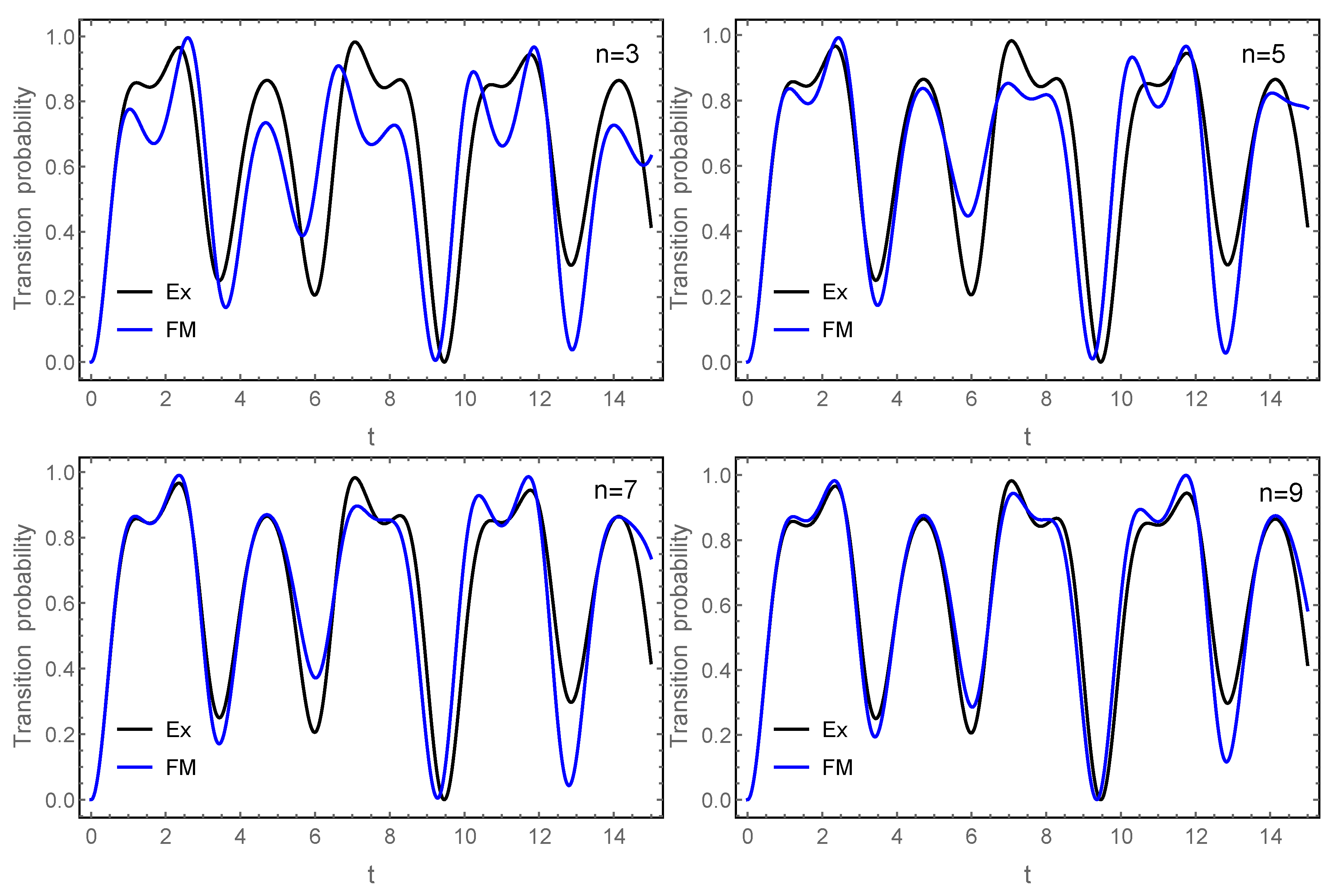
We have seen, in particular, that for problems with a periodic time dependence, the Floquet–Magnus expansion leads to more accurate results over longer time intervals, even for perturbed problems of the form A ( t ) = A 0 + ε A 1 ( t ) in the interaction picture, unless the parameter ε is exceedingly small, in which other purely perturbative procedures are competitive. It would be interesting to check whether this conclusion remains valid for more involved problems.
The interested reader may find useful the file available in [41] containing the Mathematica implementation of the techniques exposed here for the quantum mechanical problem describing the Bloch–Siegert dynamics.
In this paper we have always taken X ( 0 ) = x ( 0 ) = x 0 , but it is clear that we can also take instead X ( 0 ) as the image by the transformation of x 0 . In that case, the solution is factorized as
x ( t ) = exp ( Ω ( t ) ) exp ( t F ) X ( 0 ) = exp ( Ω ( t ) ) exp ( t F ) exp ( Ω ( 0 ) ) x 0 ,
where, obviously, the recurrences for determining Ω ( t ) and F are slightly different from those collected here. The final results can also vary, as shown in [33].
Although only examples of quantum mechanics have been considered here, the formalism of this paper can be applied in fact to any explicitly time-dependent linear system of differential equations. This might include the treatment of open quantum systems described by a non-Hermitian Hamiltonian operator [42]. This will be the subject of future research.

Author Contributions

Investigation, Software, Writing-original draft, Writing-review & editing: A.A., F.C., C.C. All authors have read and agreed to the published version of the manuscript.

Funding

This research has been funded by Ministerio de Economía, Industria y Competitividad (Spain) through project MTM2016-77660-P (AEI/FEDER, UE) and by Universitat Jaume I (projects UJI-B2019-17 and GACUJI/2020/05).

Conflicts of Interest

The authors declare no conflict of interest.

Appendix A

In this appendix we solve the equation
Ω ˙ n + [ Ω n , A 0 ] = F n F n ,
with initial condition Ω n ( 0 ) = 0 and where F n ( t ) is a quasi-periodic function
F n ( t ) = k Z r f n , k e i ( k , ω ) t ,
in such a way that F n is constant and Ω n ( t ) is quasi-periodic with the same frequencies as F n ( t ) .
First we compute the limiting mean value of F n ( t ) ,
F n lim T 1 T 0 T F n ( t ) d t
and then the antiderivative
M n ( t ) = e t ad A 0 F n ( t ) F n d t .
Then, a direct computation show that
F n = F n ( t ) [ A 0 , M n ( 0 ) ] , Ω n ( t ) = M n ( 0 ) + e t ad A 0 M n ( t )
provides the solution of (A1). To show that Ω n ( t ) is indeed quasi-periodic, we proceed as follows. First, it is clear that
F n ( t ) F n = k Z r \ { 0 } f n , k e i ( k , ω ) t
and thus
M n ( t ) = d t k Z r \ { 0 } e t ad A 0 f n , k e i ( k , ω ) t = d t k Z r \ { 0 } e t ad A 0 + i ( k , ω ) t I f n , k = d t k Z r \ { 0 } e t ad A 0 + i ( k , ω ) t I ( ad A 0 + i ( k , ω ) I ) g n , k = k Z r \ { 0 } e t ad A 0 + i ( k , ω ) t I g n , k = e t ad A 0 k Z r \ { 0 } g n , k e i ( k , ω ) t ,
where g n , k is the unique solution of the linear system consisting of d 2 equations
ad A 0 + i ( k , ω ) I X = f n , j .
In that case,
Ω n ( t ) = M n ( 0 ) + k Z r \ { 0 } g n , k e i ( k , ω ) t
is clearly a quasi-periodic function with the same basic frequencies as F n ( t ) . On the other hand, the system (A5) has a unique solution if and only if X = 0 is the unique solution of
ad A 0 + i ( k , ω ) I X = A 0 X + X ( A 0 + i ( k , ω ) I ) = 0 ,
and this happens when A 0 and A 0 + i ( k , ω ) I do not have common characteristic values, or equivalently when λ λ m i ( k , ω ) 0 for all , m { 1 , , s } , where { λ j } j = 1 s denote the distinct eigenvalues of A 0 . To avoid the problem of small divisors, a diophantine condition is introduced, namely one assumes that
| λ λ m i ( k , ω ) | > δ | k | γ , m { 1 , , s } k Z r \ { 0 }
for some constants δ > 0 and γ > r 1 , see [20,43,44] for more details. Here | k | = | k 1 | + + | k r | .
Notice that both F n and Ω n ( t ) in (A3) depend on the constant of integration M n ( 0 ) . One way of fixing it is to solve Equation (A5) and substitute g n , k into the expression of M n ( t ) . In any case, it is worth mentioning a remarkable property of the Equation (A1), namely if we have one solution F n and Ω n ( t ) , then we can get infinite solutions of the form
F ˜ n = F n + [ A 0 , R ] , Ω ˜ n ( t ) = Ω n ( t ) + R ,
where R is an arbitrary constant matrix. If we choose R = M n ( 0 ) , then
F ˜ n = F n ( t ) , Ω ˜ n ( t ) = e t ad A 0 M n ( t ) ,
so that Ω ˜ n ( 0 ) = M n ( 0 ) and one has the factorization
x ( t ) = exp ( Ω ( t ) ) exp ( t F ) X ( 0 ) = exp ( Ω ( t ) ) exp ( t F ) exp ( Ω ( 0 ) ) x 0
for the solution of (2).

References

  1. Ernst, R.R.; Bodenhausen, G.; Wokaun, A. Principles of NMR in One and Two Dimensions; Clarendon Press: Oxford, UK, 1986. [Google Scholar]
  2. Mehring, M.; Weberruss, V. Object-Oriented Magnetic Resonance; Academic Press: London, UK, 2001. [Google Scholar]
  3. Slichter, C.P. Principles of Magnetic Resonance, 3rd ed.; Springer-Verlag: Berlin, Germany, 1990. [Google Scholar]
  4. Eckardt, A. Atomic quantum gases in periodically driven optical lattices. Rev. Mod. Phys. 2017, 89, 011004. [Google Scholar] [CrossRef] [Green Version]
  5. Oka, T.; Kitamura, S. Floquet engineering of quantum materials. Annu. Rev. Condens. Matter Phys. 2019, 10, 387–408. [Google Scholar] [CrossRef] [Green Version]
  6. Hale, J. Ordinary Differential Equations; Krieger Publishing Company: Malabar, FL, USA, 1980. [Google Scholar]
  7. Mananga, E.; Charpentier, T. On the Floquet–Magnus expansion: Applications in solid-state nuclear magnetic resonance and physics. Phys. Rep. 2016, 609, 1–50. [Google Scholar] [CrossRef]
  8. Goldman, N.; Dalibard, J. Periodically driven quantum systems: Effective Hamiltonians and engineered gauge fields. Phys. Rev. X 2014, 4, 031027. [Google Scholar] [CrossRef] [Green Version]
  9. Maricq, M.M. Application of average Hamiltonian theory to the NMR of solids. Phys. Rev. B 1982, 25, 6622–6632. [Google Scholar] [CrossRef]
  10. Casas, F.; Oteo, J.A.; Ros, J. Floquet theory: Exponential perturbative treatment. J. Phys. A Math. Gen. 2001, 34, 3379–3388. [Google Scholar] [CrossRef]
  11. Lubich, C. From Quantum to Classical Molecular Dynamics: Reduced Models and Numerical Analysis; European Mathematical Society: Zürich, Switzerland, 2008. [Google Scholar]
  12. Blanes, S.; Casas, F. A Concise Introduction to Geometric Numerical Integration; CRC Press: London, UK, 2016. [Google Scholar]
  13. Hairer, E.; Lubich, C.; Wanner, G. Geometric Numerical Integration. Structure-Preserving Algorithms for Ordinary Differential Equations, 2nd ed.; Springer-Verlag: Berlin, Germany, 2006. [Google Scholar]
  14. Magnus, W. On the exponential solution of differential equations for a linear operator. Commun. Pure Appl. Math. 1954, VII, 649–673. [Google Scholar] [CrossRef]
  15. Iserles, A.; Munthe-Kaas, H.; Nørsett, S.; Zanna, A. Lie-group methods. Acta Numer. 2000, 9, 215–365. [Google Scholar] [CrossRef] [Green Version]
  16. Haga, T. Divergence of the Floquet–Magnus expansion in periodically driven one-body system with energy localization. Phys. Rev. E 2019, 100, 062138. [Google Scholar] [CrossRef] [Green Version]
  17. Casas, F.; Oteo, J.A.; Ros, J. Unitary transformations depending on a small parameter. Proc. R. Soc. A 2012, 468, 685–700. [Google Scholar] [CrossRef]
  18. Nemytskii, V.V.; Stepanov, V.V. Qualitative Theory of Differential Equations; Dover: Mineola, NY, USA, 1989. [Google Scholar]
  19. Afzal, M.; Ismaeel, T.; Jamal, M. Reducible problem for a class of almost-periodic non-linear Hamiltonian. J. Inequal. Appl. 2018, 2018, 199. [Google Scholar] [CrossRef] [PubMed]
  20. Jorba, A.; Ramírez-Ros, R.; Villanueva, J. Effective reducibility of quasi-periodic linear equations close to constant coefficients. SIAM J. Math. Anal. 1997, 28, 178–188. [Google Scholar] [CrossRef] [Green Version]
  21. Jorba, A.; Simó, C. On the reducibility of linear differential equations with quasiperiodic coefficients. J. Differ. Equ. 1992, 98, 111–124. [Google Scholar] [CrossRef] [Green Version]
  22. Palmer, K.J. On the reducibility of almost periodic systems of linear differential equations. J. Differ. Equ. 1980, 36, 374–390. [Google Scholar] [CrossRef] [Green Version]
  23. Arnold, V.; Kozlov, V.; Neishtadt, A.I. Mathematical Aspects of Classical and Celestial Mechanics, 3rd ed.; Springer: Berlin, Germany, 2006. [Google Scholar]
  24. Deprit, A. Canonical transformations depending on a small parameter. Celest. Mech. 1969, 1, 12–30. [Google Scholar] [CrossRef]
  25. Hori, G. Theory of general perturbations with unspecified canonical variables. Publ. Astron. Soc. Jpn. 1966, 18, 287–296. [Google Scholar]
  26. Blanes, S.; Casas, F.; Oteo, J.; Ros, J. The Magnus expansion and some of its applications. Phys. Rep. 2009, 470, 151–238. [Google Scholar] [CrossRef] [Green Version]
  27. Dragt, A.; Forest, E. Computation of nonlinear behavior of Hamiltonian systems using Lie algebraic methods. J. Math. Phys. 1983, 24, 2734–2744. [Google Scholar] [CrossRef]
  28. Arnal, A.; Casas, F.; Chiralt, C. A general formula for the Magnus expansion in terms of iterated integrals of right-nested commutators. J. Phys. Commun. 2018, 2, 035024. [Google Scholar] [CrossRef]
  29. Begzjav, T.K.h.; Eleuch, H. Magnus expansion applied to a dissipative driven two-level system. Results Phys. 2020, 17, 103098. [Google Scholar] [CrossRef]
  30. Verdeny, A.; Puig, J.; Mintert, F. Quasi-periodically driven quantum systems. Z. Naturforsch. 2016, 71, 897–907. [Google Scholar] [CrossRef] [Green Version]
  31. Corduneanu, C. Almost Periodic Functions; John Wiley & Sons: Hoboken, NJ, USA, 1968. [Google Scholar]
  32. Burd, V. Methods of Averaging for Differential Equations on an Infinite Interval; Chapman & Hall/CRC Press: London, UK, 2007. [Google Scholar]
  33. Arnal, A.; Casas, F.; Chiralt, C. A perturbative algorithm for quasi-periodic linear systems close to constant coefficients. Appl. Math. Comput. 2016, 273, 398–409. [Google Scholar]
  34. Scherer, W. Quantum Averaging. Habilitationsschrift, TU Clausthal, Clausthal-Zellerfeld, Germany, June 1996. [Google Scholar]
  35. Scherer, W. New perturbation algorithms for time-dependent quantum systems. Phys. Lett. A 1997, 233, 1–6. [Google Scholar] [CrossRef]
  36. Daems, D.; Guérin, S.; Jauslin, H.; Atabek, O. Pulse-driven quantum dynamics beyond the impulsive regime. Phys. Rev. A 2004, 69, 033411. [Google Scholar] [CrossRef] [Green Version]
  37. Daems, D.; Guérin, S.; Jauslin, H.; Keller, A.; Atabek, O. Optimized time-dependent perturbation theory for pulse-driven quantum dynamics in atomic or molecular systems. Phys. Rev. A 2003, 68, 051402(R). [Google Scholar] [CrossRef] [Green Version]
  38. Sugny, D.; Keller, A.; Atabek, O. Time-dependent unitary perturbation theory for intense laser-driven molecular orientation. Phys. Rev. A 2004, 69, 043407. [Google Scholar] [CrossRef] [Green Version]
  39. Pechukas, P.; Light, J.C. On the exponential form of time-displacement operators in quantum mechanics. J. Chem. Phys. 1966, 44, 3897–3912. [Google Scholar] [CrossRef]
  40. Giscard, P.-L.; Bonhomme, C. General solutions for quantum dynamical systems driven by time-varying Hamiltonians: Applications to NMR. arXiv 2020, arXiv:1905.04024v3. [Google Scholar]
  41. Arnal, A.; Casas, F.; Chiralt, C. Exponential perturbative expansions: A Mathematica code for the Bloch–Siegert Hamiltonian. Available online: http://www.gicas.uji.es/Research/EPE-VT/VarTransf.nb (accessed on 13 August 2020).
  42. Eleuch, H.; Rotter, I. Nearby states in non-Hermitian quantum systems I: Two states. Eur. Phys. J. D 2015, 69, 229. [Google Scholar] [CrossRef] [Green Version]
  43. Braaksma, B.; Broer, H. On a quasiperiodic Hopf bifurcation. Ann. Inst. Henri Poincaré Anal. Non Linéaire 1987, 4, 115168. [Google Scholar] [CrossRef] [Green Version]
  44. Broer, H. Resonance and fractal geometry. Acta Appl. Math. 2012, 120, 61–86. [Google Scholar] [CrossRef] [Green Version]
Figure 1. Transition probability for the three-lambda system with f ( t ) = e i ω t for ω = 10 ( 1 + 2 2 ) 1 2 obtained with Floquet–Magnus (FM) with n = 3 (left) and n = 4 (right) terms in the expansion. Blue line corresponds to FM, orange (Ef) line stands for the effective Hamiltonian H ef i F and black (Ex) line is the exact solution.
Mca 25 00050 g001
Figure 2. Top: transition probability for the three-lambda system with f ( t ) = e i ω t obtained with Floquet–Magnus (blue line) and Magnus expansion (red line), both with n = 3 terms. Left diagram is for ω = 6 , right diagram is for ω = 12 . Bottom: error (in logarithmic scale) as a function of time for Floquet–Magnus with n = 3 and n = 7 terms, and the effective solution with n = 7 terms (purple).
Mca 25 00050 g002
Figure 3. Error (in logarithmic scale) in the transition probability (in logarithmic scale) for the quasi-periodic case (30) as a function of time for FM (left) and Magnus (right) with n = 2 and n = 3 terms in the expansion. In both cases ω = 12 in (30).
Mca 25 00050 g003
Figure 4. Detail of Figure 3 right in the interval ω t [ 0 , 30 ] . We have included up to n = 6 terms in the Magnus series.
Mca 25 00050 g004
Figure 5. Transition probability obtained with FM (left, blue line) and LD (right, green line) with n = 3 terms in comparison with the exact result for the Bloch–Siegert Hamiltonian with ε = 0.2 (top) and ε = 1 (bottom). Black line corresponds to the exact solution, and orange to the result achieved with the effective Hamiltonian. On the right panels, the results achieved by the algorithm removing the perturbation are also depicted ( F = A 0 ).
Mca 25 00050 g005
Figure 6. Transition probability obtained with the standard Magnus expansion with n = 3 terms (red line) in comparison with the exact result (black line) for the Bloch–Siegert Hamiltonian with ε = 0.2 (left) and ε = 1 (right).
Mca 25 00050 g006
Figure 7. Transition probability obtained with FM (solid blue line) with n = 3 , 5 , 7 , 9 terms (left to right, top to bottom) in comparison with the exact result (black line) for the Bloch–Siegert Hamiltonian with ε = 1.5 .
Mca 25 00050 g007
Figure 8. Error (in logarithmic scale) in the transition probability committed by FM (left) and LD (right) with n = 3 , 5 , 7 , 9 terms each for the Bloch-Siegert Hamiltonian with ε = 0.5 . Notice the different time interval in each panel.
Mca 25 00050 g008

