Article

ssMousetrack—Analysing Computerized Tracking Data via Bayesian State-Space Models in R

by
Antonio Calcagnì
*,
Massimiliano Pastore
and
Gianmarco Altoé
Department of Developmental and Social Psychology, University of Padova, Via 8 Febbraio, 2, 35122 Padova, Italy
*
Author to whom correspondence should be addressed.
Math. Comput. Appl. 2020, 25(3), 41; https://doi.org/10.3390/mca25030041
Submission received: 23 May 2020 / Revised: 8 July 2020 / Accepted: 8 July 2020 / Published: 9 July 2020

Abstract

:
Recent technological advances have provided new settings to enhance individual-based data collection and computerized-tracking data have became common in many behavioral and social research. By adopting instantaneous tracking devices such as computer-mouse, wii, and joysticks, such data provide new insights for analysing the dynamic unfolding of response process. ssMousetrack is a R package for modeling and analysing computerized-tracking data by means of a Bayesian state-space approach. The package provides a set of functions to prepare data, fit the model, and assess results via simple diagnostic checks. This paper describes the package and illustrates how it can be used to model and analyse computerized-tracking data. A case study is also included to show the use of the package in empirical case studies.

1. Introduction

Recent technological advances allow the collection of detailed data on ratings, attitudes, and choices during behavioral tasks. Unlike standard surveys and questionnaires, these tools provide a rich source of data as they adopt tracking devices that collect subject-based information about the dynamics involved during the data collection task [1,2]. Examples of such devices include eye-tracking, body movement-tracking, computer mouse-tracking, and electrodermal activity. Among these, computer mouse-tracking has become an important and widely used tool in behavioral sciences, as it provides a valid and cost-effective way to measure the usually unknown processes underlying human ratings and decisions [3]. In a typical mouse-tracking task, individuals are presented with a computer-based interface showing the stimulus at the bottom of the screen (e.g., the image of a “dolphin”) and two labels on the left and right top corners (e.g., the labels “mammal” vs. “fish”). They are asked to decide which of the two labels is appropriate given the task instruction and stimulus (e.g., to decide whether dolphin is mammal or fish). In the meanwhile, the x-y trajectories of the computer device are instantaneously recorded. The real-time trajectories offer an effective way to study the decision process underlying the hand movement behavior by revealing, for instance, the presence of some levels of decisional uncertainty. Figure 1 shows a graphical exemplification of this task. The applications of mouse-tracking tools spread across many research area, including cognitive sciences [4], neuroscience [5], neurology [6], and forensic studies [7].
Several tools for running mouse-tracking analyses are available in open-source specialized software like MouseTracker [1], EMOT [8], and mousetrap [9]. In the R environment, only the packages mousetrack [10] and mousetrap [11] are devoted to mouse-tracking data. More generally, there are other packages developed to handle with tracking data such as trajectories [12], trackeR [13], adehabtatLT [14], and move [15]. Similarly, there are many packages developed for state-space models like, for instance, KFAS [16], bssm [17], pomp [18], and rbi [19].
In this paper, we present ssMousetrack, a novel R package to analyse computerized tracking data as they emerge from typical mouse-tracking data recording. The package implements a non-linear state space model to handle with the dynamics of mouse-tracking data which has been described in Reference [20]. In this manuscript, we describe the library ssMousetrack from a point of view of its implementation and we refer the reader to References [3,20] for further theoretical and formal issues underlying the statistical model implemented in ssMousetrack. Still, a balanced discussion of advances and limits of the proposed approach has also been proposed in Reference [20]. The model is estimated using approximated Kalman filter coupled with Markov Chain Monte Carlo (MCMC) algorithms via the rstan package [21]. The package includes functions for data pre-processing, data generation, and model assessment. It also provides functionalities to set-up designs for mouse-tracking data recording. Despite other R packages are available in this context, ssMousetrack differs in some aspects. For instance, mousetrack and mousetrap focus on descriptive evaluation of mouse-tracking data static measures (e.g., minima, maxima, flips, curvature). Among others, mousetrap also allows for clustering of trajectories based on their geometric shapes and specialized visualization functions like heatmaps and riverbed plots. By contrast, our package (i) implements a dynamic evaluation of the trajectory data without resorting the use of summary measures and (ii) evaluates the observed data variability in terms of latent dynamics and external covariates (e.g., experimental variables), which are usually of relevance in mouse-tracking data analysis. With respect to KFAS and bssm, our package offers a more focused implementation for mouse-tracking data. For instance, with regards to bssm, the package does offer an implementation for the Von-Mises distribution which is instead not supported by bssm. Moreover, although complete and useful in many cases, these packages implement a general class of state-space representations which may not be widely applicable to computerized tracking data. Finally, ssMousetrack differs also from trajectories, trackeR, adehabtatLT, and move as they focus on animal tracking and related problems, such as estimation of habitat choices. This makes them not directly suitable for analysing the various aspects of mouse-tracking studies. In this respect, the advantages of ssMousetrack are as follows: (i) it is easy to use as it requires typing a single function to run the entire procedure, (ii) it allows modeling and analysing computerized tracking data as they are usually recorded in typical mouse-tracking tasks, (iii) it provides a user-friendly workflow for all processing steps which can be easily understood by non-expert users, (iv) it offers users a way to simulate mouse-tracking designs and data as well. In addition, ssMousetrack can be combined with other R packages, including shinystan [22] and ggmcmc [23] to produce further statistical and graphical representation of the output. The package is available from the Comprehensive R Archive Network at https://CRAN.R-project.org/package=ssMousetrack.
This paper is organized as follows. Section 2 gives a statistical overview of the model implemented in the package, the methods of estimation and inference, and the assessment of the model. Section 3 describes the package’s structure and its utilities. Section 4 illustrates the functioning of the package by means of an illustrative case study. Finally, Section 5 concludes the manuscript with a discussion and future directions.

2. Model

In this section, we will briefly illustrate the model implemented in the current version of ssMousetrack. Further technical details and theoretical issues about the model’s representation can be found in Reference [20]. Moreover, a more general introduction to the problem of modeling mouse-tracking trajectories from a cognitive viewpoint can be found in Reference [3]. In mouse-tracking studies, computerized mouse-tracking data typically consist of arrays ( x , y ) i j R N i j × R N i j containing the streaming of x-y Cartesian coordinates of the computer-mouse pointer, for i = 1 , , I subjects, j = 1 , , J stimuli, and n = 1 , , N i j time steps. To simplify data analysis, raw trajectories are usually pre-processed according to the following steps [8,24]. First, the trajectories ( x , y ) i j are normalized on a common sampling scale such that N is the same over subjects and stimuli. Next, the arrays ( x , y ) i j R N × R N are rotated and translated into the quadrant [ 1 , 1 ] × [ 1 , 1 ] with ( x 0 , y 0 ) i j = ( 0 , 0 ) and ( x N , y N ) i j = ( 1 , 1 ) by convention. Finally, normalized data are projected onto a (lower) 1-dimension space via atan2 function. In this way, the final ordered data y i j = y ( 1 ) , , y ( n ) , , y ( N ) ( 0 , π ] N lie on the arc defined by the union of two disjoint sets, that is, the set { y ( 0 , π ] : y π 2 } which represents the right-side section of the screen (usually called target, T) and the set { y ( 0 , π ] : y < π 2 } which instead represents the left-side section (usually called distractor, D). The final data are arranged as an Y N × J I column-wise stacked matrix.
The state-space model implemented in ssMousetrack is as follows:
y J I × 1 ( n ) vonMises μ J I × 1 ( n ) , κ J I × 1 ( n )
μ J I × 1 ( n ) = G x I × 1 ( n ) , β J × 1
x I × 1 ( n ) Normal x I × 1 ( n 1 ) , σ x I I × I
β J × 1 = Z J × K · γ K × 1
κ J I × 1 ( n ) = exp λ d J I × 1 ( n ) ,
where Equation (1) is a von Mises measurement equation with μ J I × 1 ( n ) ( 0 , π ] I J being the mean for the n-th time step and κ J I × 1 ( n ) R I J the concentrations around the n-th mean vector, Equation (2) represents the locations on the arc defined in ( 0 , π ] from which the data vector y ( n ) is sampled from and it behaves according to the a real function G : R ( 0 , π ] , which maps reals into radians. In the current version of ssMousetrack, G can be defined as:
(i)
π -scaled logistic function:
G = vec π 1 1 + exp β J × 1 1 1 × I 1 J × 1 x 1 × I ( n ) )
with β J × 1 R J representing the contribution of the stimuli on y ( n ) .
(ii)
π -scaled Gompertz function:
G = vec π exp β J × 1 1 1 × I exp 1 J × 1 x 1 × I ( n ) ,
where β J × 1 R + J has the same meaning as before.
Although they represent two cases of the general family of S-shaped functions, logistic and Gompertz models differ in some respects. For instance, unlike the logistic model, the Gompertz function is not symmetric around its inflection point, with the consequence that its growth rises rapidly to its maximum rate occurring before the fixed inflection point [25]. Moreover, the parameters of the Gompertz function are always positive, a constrain which is often required by applications where the covariates of the model cannot take negative values (e.g., reaction times). These two implementations allow users to choose the type of G function on the basis of the experimental designs they have used in their studies.
Equation (3) represents a Normal states equation in the form of a lag-1 autoregressive process with time-fixed variance parameter σ x . In the current version of ssMousetrack, the covariance matrix of the latent processes is set to an identity matrix I without loss of generality ( σ x = 1 ). Equation (4) is the linear term modeling the contribution of the experimental design (e.g., two-by-two design) and variables involved (e.g., categorical variables, continuous covariates). Note that Z is a design (dummy) matrix of main and high-order effects defined by adopting the dummy coding (e.g., treatment contrasts, sum contrasts) whereas γ is the associated vector of parameters for the columns of Z , with γ 1 being the usual baseline term for the contrasts. Finally, Equation (5) defines the concentrations around the n-th location by using the transformed data:
d ( n ) = | y ( n ) 3 π 4 | , if y ( n ) < π 2 | y ( n ) π 4 | , if y ( n ) π 2 ,
with exp : ( 0 , π ] [ lb , ub ] R + being the exponential function scaled in the natural range of the concentration parameter (e.g., l b = 10 , u b = 200 ). In the current implementation of the package, the parameter λ is fixed to unity.
The interpretation of Equations (2)–(4) is as follows. The n-th mean vector μ ( n ) is expressed as function of the stimuli-related component β and subject-based component x ( n ) , which are integrated together to form the conditional sampling y ( n ) | β , x ( n ) through the function G . As a result, Equation (3) can be interpreted as the individual latent dynamics that are unaffected by the experimental stimuli whereas Equation (4) represents the experimental effect regardless to individual dynamics. More generally, Equation (3) conveys information about the hand movement process underlying the tracking device and as such it can be used to analyse how much individuals differ in executing the task. By contrast, Equation (4) collects information on how a certain experimental manipulation has an effect or not on the movement responses. Interestingly, when normalized into [ 0 , 1 ] , μ ( n ) can be interpreted as the probability of the i-th individual at the j-th stimulus to navigate close the distractor cue in the left-side section of the arc. Finally, Equation (5) follows from the fact that hand movements underlying computerized tracking data tend to be smooth over the experimental task, with small changes being more likely close to left (distractor) or right (target) endpoints [26].

2.1. Estimation and Inference

The state-space model in Equations (1)–(5) requires estimating the array of latent trajectories X R I × N together with the array of parameters γ K × 1 , with γ 1 R and γ ( K 1 ) × 1 R K 1 (logistic case) or γ ( K 1 ) × 1 [ γ 1 , ) K 1 (Gompertz case). The array of unknown quantities Θ = { X , γ } can be estimated in various way, by adopting both a frequentist and Bayesian perspectives [27]. In the ssMousetrack package, the parameters are recovered in Bayesian way by means of MCMC algorithm through which X and γ are alternately recovered [28,29]. The reason is twofold: (i) MCMC algorithms, as those implemented in rstan package, provide a more efficient solution for sampling from the probability distribution of the parameters over standard maximum-likelihood based approach such as the Expectation-Maximization algorithm. (ii) The Bayesian approach offers an elegant solution for data analysis and inference [30] by means of which the model is adequately assessed by the analysis of (marginal) posterior distributions of the parameters [31].
More in details, the posterior density f ( Θ | Y ) after factorization of the joint density f ( γ , X , Y ) , is as follows [28]:
f ( Θ | Y ) f ( γ ) f ( γ | Y ) f ( X | Y ) ,
where f ( γ | Y ) is the (marginal) likelihood function, f ( X | Y ) is the filtering density, whereas f ( γ ) is the prior ascribed on the model parameters. In the current version of ssMousetrack, f ( X | Y ) is approximated via Kalman filtering/smoothing, with f ( γ | Y ) being computed as a byproduct of the Kalman theory (see Appendix A and Reference [32]). It should be noted that the Kalman filter adopted here provides an approximation to the estimate of the latent states given the observed data. Likewise for the more general extended Kalman filter, the quality of the filtering approximation relies upon the Gaussian approximation of the von-Mises measurement equation (e.g., see Reference [29], ch. 5). Since the states equation of our model is Gaussian (Equation (3)), nonlinearities enter the model only through Equation (2) which shrinks the domain of the latent states onto the subset ( 0 , π ) . The measurement equation uses the Von-Mises distribution, which is a wrapped approximation of the Gaussian density on the circle, with the approximation being better for larger κ J I × 1 [33]. In this sense, the Kalman filter implemented in ssMousetrack uses the Normal approximation to the von-Mises distribution while using the nonlinear transformation of the measurements into the update step (e.g., see Reference [29], ch. 5). In doing so, an update of the variance for the latent states uses the approximation 1 / κ J I × 1 = 1 / exp ( λ d J I × 1 ( n ) ) for the variance of the measurements. Similarly, an update of the mean for the latent states requires the term y J I × 1 G x ^ I × 1 ( n ) , Z J × K · γ K × 1 , with G being defined as in Equation (2), which allows the difference between observed and predicted measurements to be defined on the same domain ( 0 , π ) . The optimality of the approximation is guaranteed as long as the Normal approximation to the Von-Mises holds, in particular for larger values of κ J I × 1 . In the context of mouse-tracking data, this approximation is valid until computerized mouse-tracking trajectories show small and smooth changes over the reaching task. This ensures that using concentrated von-Mises/Normal densities to predict next movements given past data is good enough to meet the requirements of mouse-tracking applications.

2.2. Model Assessment

In the Bayesian context of data analysis, ssMousetrack provides a simulation-based procedure to evaluate the adequacy of the model to reproduce the observed data Y [30]. More technically, given the posteriors of parameters and latent states f ( Θ | Y ) , M new (simulated) datasets Y 1 * , , Y M * are generated according to the estimated model structure and, for each new dataset, two discrepancy measures are considered [34]:
PA overall = 1 | | Y m Y | | 2 / | | Y | | 2
PA sbj = 1 | | Y m ( i ) Y ( i ) | | 2 / | | Y ( i ) | | 2 i = 1 , , I ,
which measure the total amount of data reconstruction based on the overall J I × N observed array Y (Equation (7)) and the amount of data reconstruction based on the J × N observed matrix Y ( i ) for each subject i = 1 , , I (Equation (8)). Both the indices are in the range 0-100%, with 100% indicating optimal fit. Note that the measure PA sbj allows for evaluating the adequacy of the model to reconstruct the individual-based set of data. In addition, the dynamic time warp distance (dtw), as implemented in dtw package, is also computed between Y m ( i ) and Y ( i ) . Unlike the PA sbj index, the dtw distance measures the similarity among time series by considering their different dynamics [35]. Note that more general methods and criteria are available in the Bayesian literature (e.g., see Reference [36]), such as graphical evaluation of the discrepancy between observed and posterior predictive statistics. In this sense, the foregoing measures—which are generally used to assess how much the predicted array of data resemble the observed arrays (e.g., see Reference [34])—here are intended to provide further measures supporting the existing ones, and do not offer an alternative way to do Bayesian model assessment. Since ssMousetrack uses rstan as backend, users can perform model assessment by means of other existing libraries, such as bayesplot [37].

3. The ssMousetrack Package

The ssMousetrack is distributed via the Comprehensive R Archive Network (CRAN). It is based on rstan [21], the R interface to the probabilistic programming language Stan [38]. The current version of the package allows for (i) simulating data according to a given experimental design, (ii) analysing mouse-tracking data via state-space modeling, and (iii) evaluating the adequacy of model results. The package consists of five main function (generate_data(), run_ssm(), check_prior(), prepare_data(), evaluate_ssm()), two datasets (language, congruency), and three sub-functions (compute_D(), generate_Z(), generate_design()). The main functions generate_data() and run_ssm() are wrappers to previously-compiled Stan codes which implement the model described in Section 2. Table 1 provides an overview of the functions and datasets provided in the ssMousetrack package whereas a description of the usage of the functions is reported in the next subsections.
The package can simply be installed via R console using the function:
install.packages("ssMousetrack")

3.1. Generate Artificial Data

To simulate artificial data we use the function generate_data(), which requires as input the experimental template for the data generation process. More generally, the function works by first sampling the parameters γ from the prior density f ( γ ) and then generates the latent states X from Equation (3), computes the matrix μ from Equation (2) and the matrix D , drawns the matrix of data Y by simply applying Equation (1). For instance, an experiment with one categorical independent variable and two levels, each with three trials, can be generated via the following syntax:
prior_list <- list("normal(-0.25,0.5)","normal(2.7,1)")
datagen1_ssm <- generate_data(N = 61, M = 100,I = 2,J = 6,
K = 2,Z.formula = "~Z1", priors = prior_list),
where M = 100 is the number of data to be generated, N = 61 is the number of time step for the mouse-tracking trajectories, K = 2 means that we have just one variable with two levels, J = 6 indicates the total number of trials such that J/K is the number of trials for each level of the variable, I = 2 is the number of subject, Z.formula indicates the formula for the contrast matrix Z with standard R syntax. Note that selective priors are specified for each level of the experimental design using the Stan syntax (see the help of check_prior() for further technical details). (Priors are allocated according to the number of model parameters implied by the design matrix Z of the linear predictor of the model. Thus, for instance, if we have two predictors in a simple additive model (no interaction), we need to specify two priors. Instead, a model with two additive predictors and the interaction between them require three priors as the number of parameters in the linear predictor is three, that is, two for the additive component and one for the interaction.)
The output is a list containing three sublists, as follows:
  • params, which contains the model parameters generated for the M datasets:
    ## List of 4
    ##  $ sigmax: num [1:2] 1 1
    ##  $ lambda: num [1:12] 1 1 1 1 1 ...
    ##  $ gamma : num [1:75, 1:2] 0.228 -0.378 ...
    ##  $ beta  : num [1:75, 1:12] 0.228 -0.378 ...
  • data, which contains the matrices of latent states X and trajectories Y , together with μ , D , and Z :
    ## List of 5
    ##  $ Y : num [1:75, 1:61, 1:12] 1.54 1.53 ...
    ##  $ X : num [1:75, 1:61, 1:2] 1e-04 1e-04 1e-04 1e-04 1e-04 ...
    ##  $ MU: num [1:75, 1:61, 1:12] 1.57 1.57 ...
    ##  $ D : num [1:75, 1:61, 1:12] 0.785 0.785 ...
    ##  $ Z : num [1:12, 1:2] 1 1 1 1 1 ...
  • design, which contains the experimental design used as template to generate the data:
    ##   sbj trial  Z1
    ## 1   1     1 100
    ## 2   1     2 100
    ## 3   1     3 100
Similarly, artificial datasets can be generated using more complex designs. For instance, a bivariate design with two variables is produced by typing:
datagen2_ssm <- generate_data(I = 2,J = 8,K = c(2,4),Z.formula = "~Z1*Z2",
Z.type=c("symmetric","random")),
where K = c(2,4) codifies two variables each with two and four levels, Z.formula = " Z1*Z2" indicates that the variables interact whereas Z.type=c("symmetric","random") indicates that trials must be assigned to the first variable using the symmetric method and to the second variable using the random method (see the help of generate_Z() for further details).
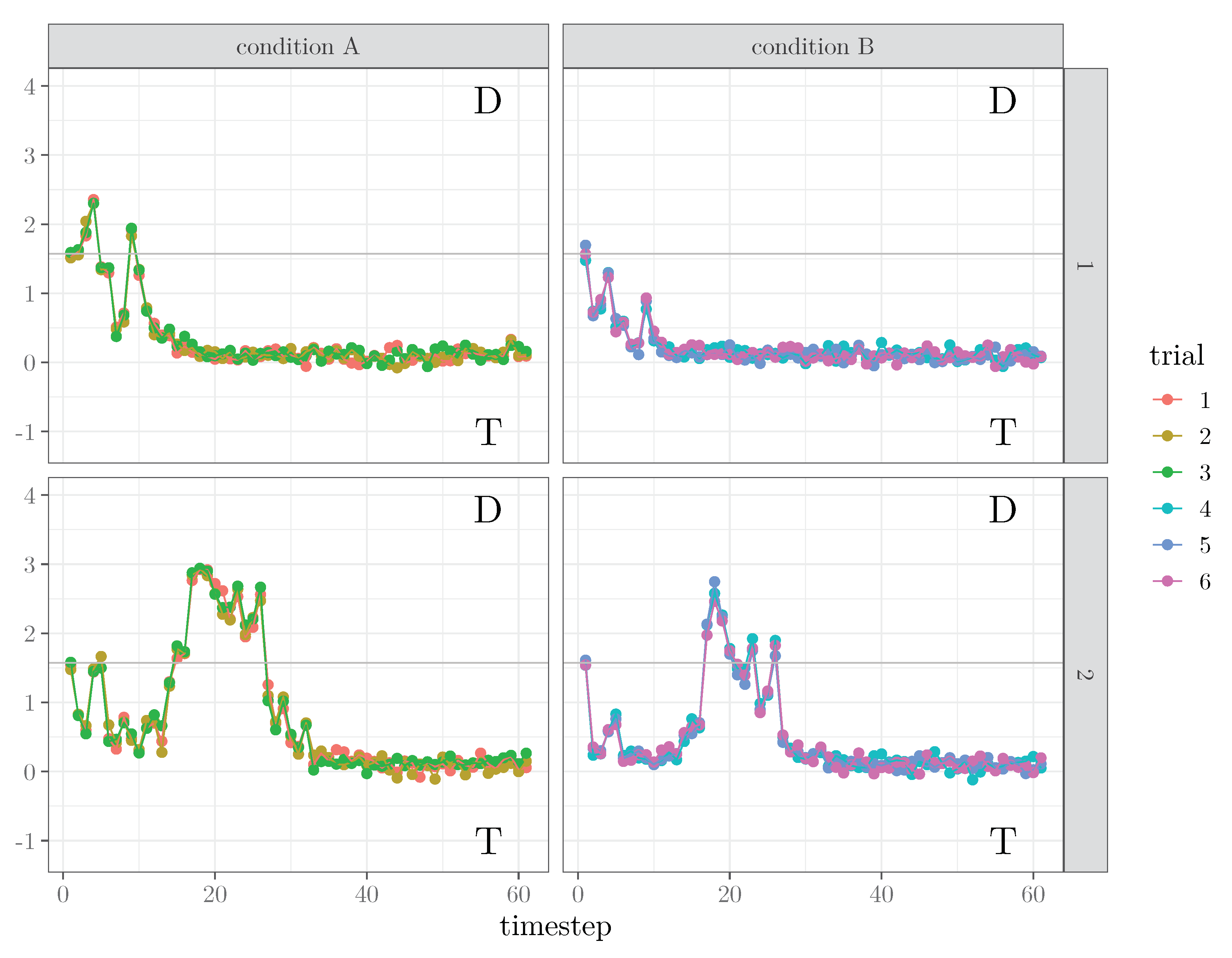
Figure 2 shows a sample of mouse-tracking data Y generated in the univariate design case with I = 2, K = 2 and J = 6. We report the univariate case only for the sake of simplicity but the same graphical representations can be done for the more complex designs as well.

3.2. Run State-Space Analysis

State-space analysis can be run on both simulated and real data. In the first case, after the data-generation process, the state-space model implemented in the ssMousetrack package can be fit using run_ssm(). For instance, the syntax:
datagen2_ssm <- generate_data(I = 2,J = 8,K = c(2,4),Z.formula = "~Z1*Z2",
Z.type=c("symmetric","random"))
iid <- 2
datagen2_fit <- run_ssm(N = datagen2_ssm$N,I = datagen2_ssm$I,
   J = datagen2_ssm$J,Y = datagen2_ssm$data$Y[iid,,],
   D = datagen2_ssm$data$D[iid,,],Z = datagen2_ssm$data$Z,
   niter = 5000,nwarmup = 2000,nchains = 2)
runs the state-space analysis on the iid = 2 artificial data datagen2_ssm. Note that niter indicates the number of total samples to be drawn, nwarmup the number of warmup/burnin iterations per chain, and nchains the number of chains to be executed in parallel. The function run_ssm() allows for parallel computing via the parallel package when nchains > 1. In this case, since ncores="AUTO" (default), the function will run two parallel chains using two cores.
Unlike for the case of artificial data, the analysis of real datasets requires preparing raw data in a proper format via prepare_data(), the function that implements the steps described in Section 2. Generally, raw datasets need to be organized using the long-format, with information being organized as nested. The dataset language is an example of a typical data structure required by prepare_data():
data("language")
str(language,vec.len=2)
## ’data.frame’: 6060 obs. of  6 variables:
##  $ sbj      : int  1 1 1 1 1 ...
##  $ trial    : int  1 1 1 1 1 ...
##  $ condition: Factor w/ 4 levels "HF","LF","PW",..: 1 1 1 1 1 ...
##  $ timestep : int  1 2 3 4 5 ...
##  $ x        : num  0 -0.0098 -0.0098 -0.0098 -0.0098 ...
##  $ y        : num  0 0.0025 0.0025 0.0025 0.0025 ...
where condition is the categorical variable involved in the study. The pre-processing of raw data is performed by the call:
language_proc <- prepare_data(X = language,N = 61,Z.formula = "~condition")
where the output language_proc is a data frame containing the pre-processed dataset together with the column-wise stacked matrix Y of angles, the contrast matrix Z , and the matrix of distances D .
Once raw data have been pre-processed, the state-space analysis is performed as for the case of artificial data:
language_fit <- run_ssm(N = language_proc$N,I = language_proc$I,
   J = language_proc$J,Y = language_proc$Y,
   D = language_proc$D,Z = language_proc$Z,
   niter = 5000,nwarmup = 2000,nchains = 2)
The function returns as output a list composed of three sublists, as follows:
  • params, which contains the posterior samples for the free parameters γ and β :
    ## List of 6
    ##  $ sigmax    : num 1
    ##  $ lambda    : num 1
    ##  $ kappa_bnds: num [1:2] 5 300
    ##  $ gamma     :’data.frame’: 4000 obs. of  4 variables:
    ##  $ beta      : num [1:4000, 1:60] -0.26 -0.146 ...
    ##  $           :function (z, ...)
  • data, which contains the posterior samples for the latent states X and the moving means μ :
    ## List of 6
    ##  $ Y       : num [1:101, 1:60] 1.56 1.7 ...
    ##  $ X       : num [1:4000, 1:101, 1:5] 1e-04 1e-04 1e-04 1e-04 1e-04 ...
    ##  $ MU      : num [1:4000, 1:101, 1:60] 1.76 1.68 ...
    ##  $ D       : num [1:101, 1:60] 0.592 0.474 ...
    ##  $ Z       : num [1:60, 1:4] 1 1 1 1 1 ...
    ##  $ X_smooth: num [1:4000, 1:101, 1:5] -0.0878 -0.0635 ...
  • stan_table, containing the typical Stan output (i.e., point estimates, credibility intervals, and Gelman–Rubin index) for the sampling() method as implemented in the rstan package:
    ##           mean se_mean   sd  2.5%   25%   50%  75% 97.5% n_eff Rhat
    ## gamma[1] -0.05       0 0.19 -0.43 -0.18 -0.05 0.08  0.33  3047    1
    ## gamma[2] -0.02       0 0.06 -0.13 -0.06 -0.02 0.02  0.09  2764    1
    ## gamma[3]  0.16       0 0.06  0.04  0.12  0.16 0.20  0.28  2782    1
Note that users can also export the stanfit object with all the Stan results by specifying stan_object=TRUE in run_ssm().
The function run_ssm() allows for different priors specification. In particular, users can specify different priors for the model parameters γ as follows:
priors_list <- list("lognormal(1,0.5)","normal(1,2)","chi_square(2)","normal(0,1)")
language_fit <- run_ssm(..., priors = priors_list)
which means that γ 1 lognormal ( 1 , 0.5 ) , γ 2 normal ( 1 , 2 ) , γ 3 chi_square ( 2 ) , γ 4 normal ( 0 , 1 ) . The list of probability distributions accepted by run_ssm() is described in the help of the function check_prior(). Specification of priors for single parameters is also allowed, by using NULL attributes:
priors_list <- list(NULL,"normal(1,2)","chi_square(2)",NULL)
language_fit <- run_ssm(..., priors = priors_list)
where predefined priors are used for parameters γ 1 and γ 4 . Further examples about run_ssm() are illustrated in the manual of the package.

3.3. Evaluate the Model Results

The methods described in Section 2.2 for the model evaluation are implemented by the function evaluate_ssm(), which requires as input the output of run_ssm(). For instance, considering the fitted object language_fit, the model evaluation can simply be run via the command:
language_eval <- evaluate_ssm(ssmfit = language_fit, M = 1000, plotx = FALSE),
where M = 1000 is the number of replications to compute the indices. The function returns as ouput a list containing the mean values of the indices PA overall , PA sbj , and dtw, as well as the distributions obtained over the M replications. Note that, users can also ask for a graphical representation of the indices by setting plotx = TRUE.

4. Application

In this section we provide a full example of the way ssMousetrack can be used for state-space analysis of real computerized tracking data. Note that the application reported here has an illustrative purpose only. To this end, we will make use of the dataset language, a subset of data originally presented in Reference [39]. In this typical computerized tracking task, participants saw a printed stimulus on the screen (e.g., the word water) and were requested to perform a dichotomous choice task where stimuli need to be classified as word or non-word. The experimental variable condition was a categorical variables with four levels (HF: High-frequency word; LF: Low-frequency word; PW: Pseudo-word; NW: Non-word). Participants had to classify each stimulus as word vs. non-word by using a computer-mouse tracking device. The dataset contains I = 5 participants, J = 12 trials, one categorical variable with K = 4 levels, each with J / K = 3 trials. From the data-analysis viewpoint, we evaluat the extent to which the parameters of the state-space model γ reflect eventual differences associated with the levels of condition.
The raw computerized tracking trajectories in the dataset consist of Cartesian coordinates with N = 101 ( i = 1 , , I ; j = 1 , , J ). The dataset is partially pre-processed as raw trajectories have the same length ( N = 101 ). However, we need to run prepare_data() in order to rotate/translate the raw data into the quadrant [ 1 , 1 ] × [ 1 , 1 ] and compute the atan2 projections. The pre-processing step is called by the command:
data("language")
language_proc <- prepare_data(X = language, N = 101, Z.formula = "~condition")
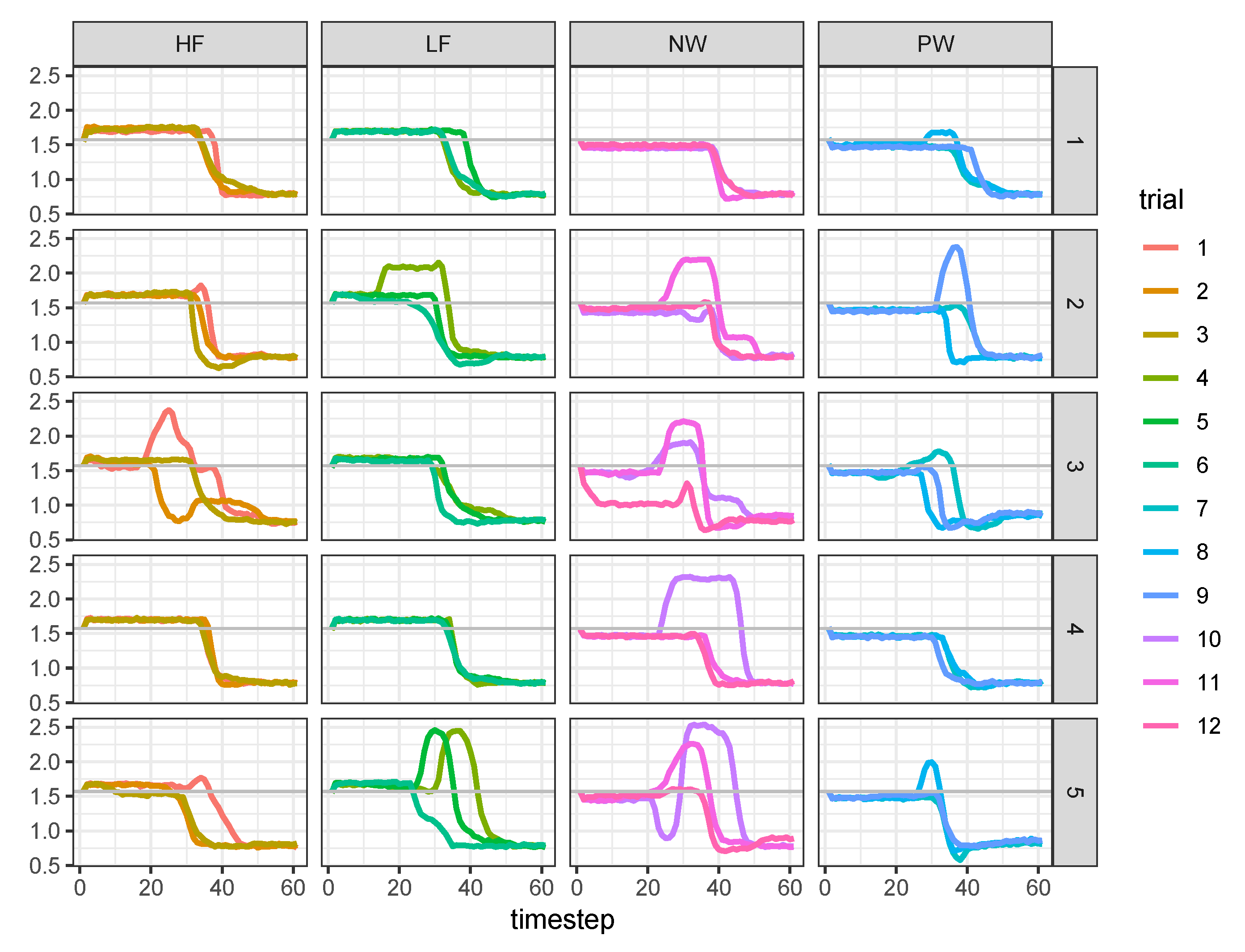
Figure 3 shows the trajectories Y associated with the task for all participants and trials.
Next, the state-space model is fit to the pre-processed data by the following call:
priors_list <- list("normal(0,1)","normal(1,1)","normal(-2,1)","normal(2,1)")
language_fit <- run_ssm(N = language_proc$N,I = language_proc$I,
J = language_proc$J,Y = language_proc$Y,
D = language_proc$D,Z = language_proc$Z,
niter = 6000,nwarmup = 2000,nchains=4,
priors = priors_list,
gfunction = "logistic")
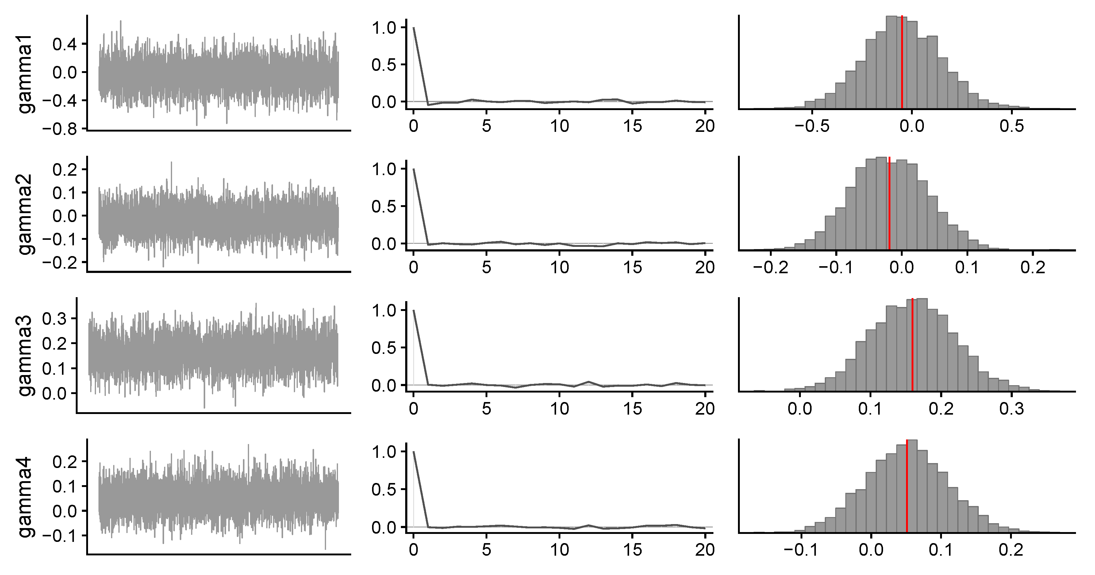
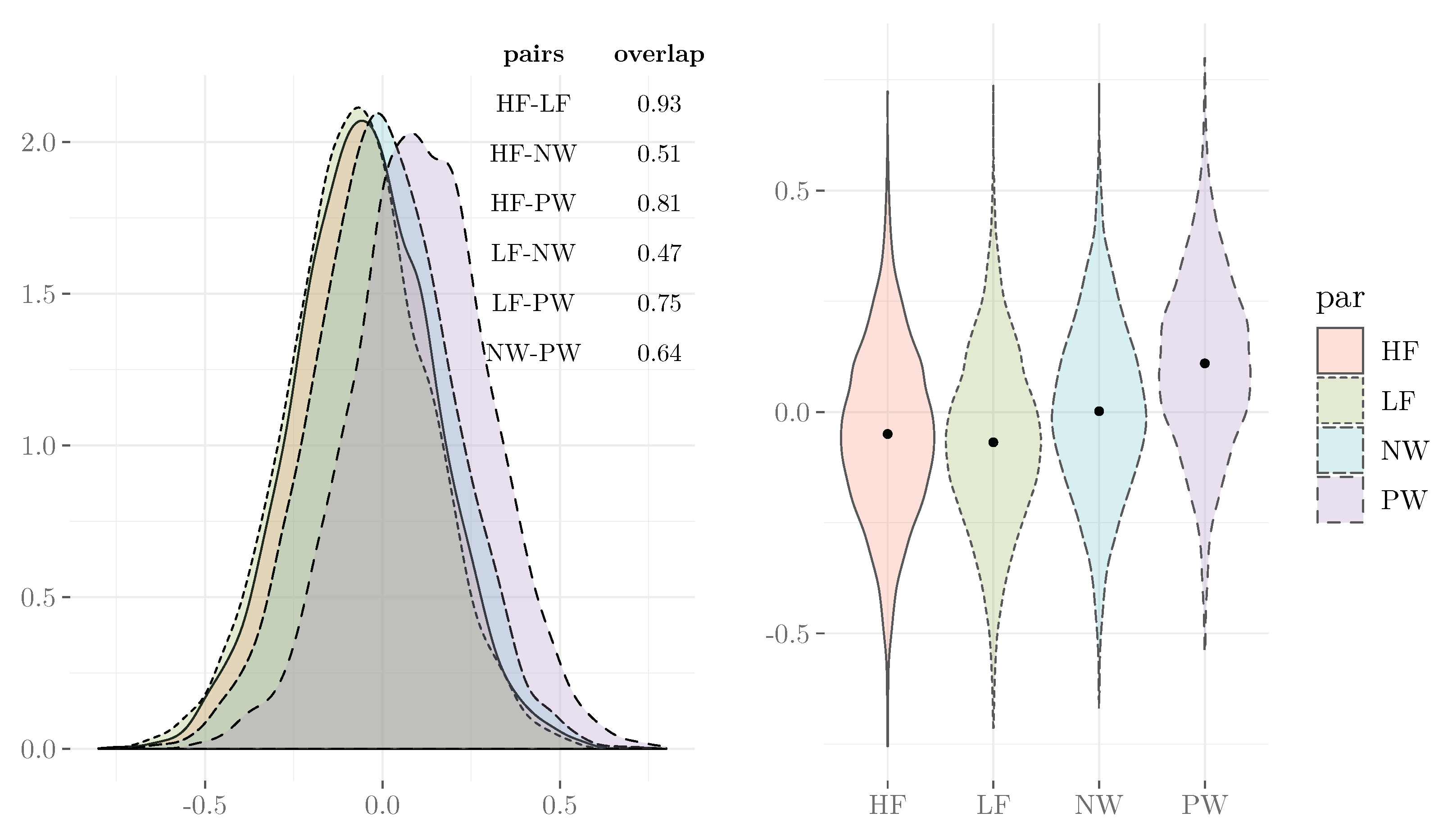
where, in this case, the prior for γ have been choosen to codify a priori expectations about the effect of the variable condition [39]. Figure 4 shows some MCMC graphical diagnostics for the model parameters γ computed using bayesplot [37] whereas Table 2 reports the posterior quantities for the model parameters. In the Bayesian context of data-analysis, we evaluate the effects of the variable condition by computing the degree of overlapping among marginal posterior densities for each level of the experimental variable (i.e., the more the overlapping, the weaker the evidence supporting the experimental manipulation). Figure 5 shows the results graphically. Overall, the variable condition showed no strong effect, as the densities of the levels are overlapped. In particular, stimuli in HF, LF, and NW conditions showed no activation of the distractor section of the tracking space as γ ^ HF , γ ^ NW , and γ ^ LF approach zero. By contrast, stimuli in PW condition showed a small effect on activating the target section ( γ ^ HF > 0 ), possibly due to the fact that PW stimuli require less cognitive workload [39].
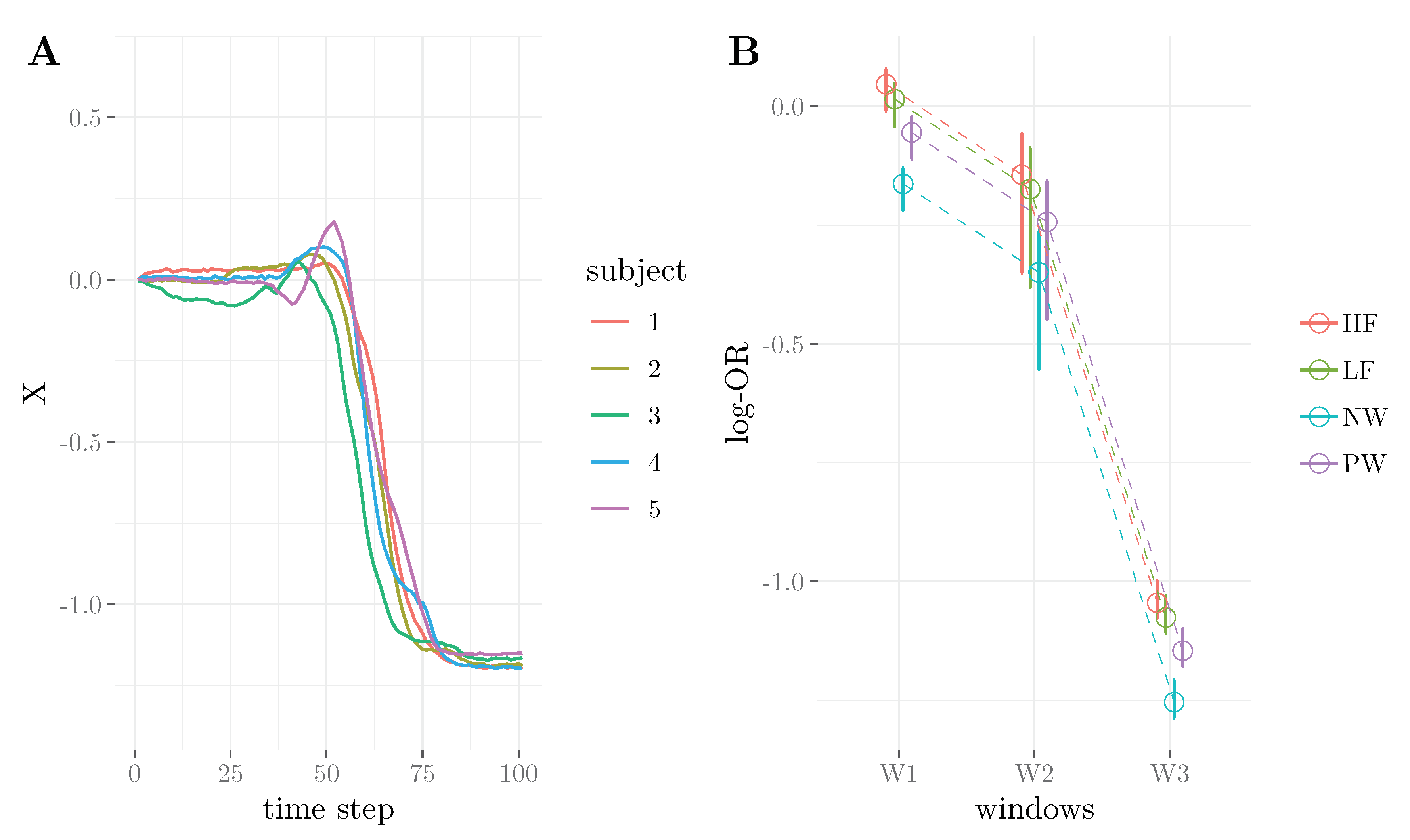
Figure 6A reports the filtered latent states X ^ for the subjects in the dataset. To further investigate how individual dynamics differ over the levels of condition, we can make use of X ^ and ask whether HF, LF, NW, and PW stimuli differ in terms of evidence of mouse-tracking competition. The idea is that the higher the evidence, the larger the difficulty in categorizing stimuli as word (target) or non-word (distractor).
To do this, we follow the findings of Reference [39] and divide the entire respose process 1 , , N into three disjoint windows W 1 = 10 35 % , W 2 = 45 65 % , and W 3 = 70 85 % . Usually it is expected that a higher competition would be observed in W 1 and W 2 rather than W 3 . More formally, let x ^ M × 1 ( i ) = ( x ^ 1 ( i ) , , x ^ M ( i ) ) be the sequence of filtered states for the i-th subject and the generic time window W, with M being equals to the cardinality of W. Next, the probability to select non-word (distractor) responses are computed by normalizing the G function into the domain [ 0 , 1 ] , as follows:
P M × K ( i ) = 1 + exp x ^ M × 1 ( i ) 1 1 × K 1 M × 1 γ ^ 1 × K 1 ,
where γ ^ is the array of posterior means of the model parameters. Note that in this example we use the logistic function because we set gfunction="logistic" in run_ssm(). Finally, the evidence measures can be defined in terms of log-odd ratio using the probability matrix P ( i ) :
r K × 1 ( i ) = log p K × 1 ( i ) / 1 p K × 1 ( i ) ,
where p K × 1 = 1 M 1 1 × M P M × K ( i ) T is the profile probability for HF, LF, NW, and PW. The interpretation of r ( i ) is as follows. For r ( i ) > 0 there is a higher competition in categorizing the stimulus as word (target) vs. non-word (distractor). By contrast, for r ( i ) < 0 there is a lower competition in the response process, as stimuli are easily categorized as word (target). Finally, the case r ( i ) = 0 indicates that there is no difference in terms of evidence between word (target) and non-word (distractor) responses. Figure 6B shows the results for the four levels of condition. As expected, the competition in the third phase of the response process W 3 is low, as the probability to select the target is higher. The same applies to W 2 . On the contrary, in the first stage of the process W 1 the competition is higher although the evidence ratio for all the levels of condition approximate zero. Interestingly, the second phase W 2 shows a higher whithin-subject variability of competition, which probably indicates that subjects differ in the categorization process just in the middle phase of the response process.
Finally, we assess the adequacy of the model with regards to the observed data by means of evaluate_ssm(), as follows:
language_fit_eval <- evaluate_ssm(ssmfit = language_fit,M = 500,plotx = FALSE)
where language_fit is the fitted object returned by run_ssm() whereas M = 500 is the number of replications used to compute the three fit indices. The output of the function consists of a list containing means and distributions of the fit indices:
## List of 2
##  $ dist   :List of 3
##   ..$ PA_ov : num [1:500] 0.944 0.938 ...
##   ..$ PA_sbj: num [1:500, 1:5] 0.991 0.991 ...
##   ..$ DTW   : num [1:500, 1:60] 0.0945 0.1105 ...
##  $ indices:List of 3
##   ..$ PA_ov : num 0.936
##   ..$ PA_sbj: num 0.99
##   ..$ DTW   : num 0.119
Overall, in this example the fitted model is adequate to reproduce the observed trajectory data as supported by high values of the indices PA ov , PA sbj , and dtw.

5. Conclusions

In this paper we introduced the R package ssMousetrack that analyses computerized-tracking data using Bayesian state-space modeling. The package provides a set of functions to facilitate the preparation and analysis of tracking data and offers a simple way to assess model fit. The package can be of particular interest to researchers needing tools to analyse computerized-tracking experiments using a complete statistical modeling environment instead of descriptive statistics only. In addition, the package ssMousetrack allows for individual-based analysis of trajectories where latent dynamics are used to obtain richer information which can pave the way to further analyses (e.g., profile analysis). The current version of the package can be extended in several ways. For instance, the inclusion of other state-space representations beyond the simple Gaussian AR(1) model can be a further generalization of the package. Still, model parameters like σ x and λ can be free to allow for multi-group analysis. Similarly, more comprehensive model diagnostics could also be considered in future releases of the package. Additionally, the current version of the library can be extended to interact with other modeling packages available on R, such as pomp [18] or libBi [41], which can be successfully used to estimate model’s parameters. Finally, it should be stressed that the method implemented in the current version of ssMousetrack produces approximate inference for the model’s parameters and exact methods, such as particle filtering based MCMC [28], may instead be used. Although they can show slower computational time when compared to approximated methods, they may improve the quality of estimates. This can constitute a future venue of our research and next versions of ssMousetrack may incorporate particle filter methods as well.
In closing, we believe our package may be a useful tool supporting researchers and practitioners who want to make analysis of computerized-tracking experiments using a statistical modeling environment. This will surely help them to improve the interpretability of data analysis as well as the reliability of conclusions they can draw from their studies.

Author Contributions

conceptualizaton, A.C.; methodology, A.C.; software, A.C., M.P., G.A.; formal analysis, A.C., M.P.; writing—original draft preparation, A.C.; writing—review and editing, A.C., G.A., M.P. All authors have read and agreed to the published version of the manuscript.

Funding

This research received no external funding.

Conflicts of Interest

The authors declare no conflict of interest.

Appendix A

Given a candidate sample γ , the mean x and variance λ of the density f ( X | Y ) are approximated via the following recursion:
( n = 0 ) x ^ I × 1 ( n ) = 0 I × 1
λ ^ I × 1 ( n ) = 1 I × 1
( n > 0 ) x ¯ I × 1 ( n ) = x ^ I × 1 ( n 1 )
λ ¯ I × 1 ( n ) = λ ^ I × 1 ( n 1 )
y ^ J I × 1 = G x ¯ I × 1 ( n ) , Z J × K · γ K × 1
σ J I × 1 = I J × J λ ¯ I × 1 ( n ) 1 J × 1 + 1 exp ( d J I × 1 ( n ) )
K J I × 1 = I J × J λ ¯ I × 1 ( n ) 1 J × 1 σ J I × 1
x ^ I × 1 ( n ) = x ¯ I × 1 ( n ) + ( y J I × 1 y ^ J I × 1 ) K J I × 1 T A J I × I T
λ ^ I × 1 ( n ) = λ ¯ I × 1 ( n ) + K J I × 1 σ J I × 1 K J I × 1 T A J I × I T
where ⊗ is the Kronecker product, ⊙ the (element-wise) Hadamard product, ⊘ the (element-wise) Hadamard division, whereas A = I I × I n 1 J × 1 is a scaling matrix with n = 1 / J . As a byproduct of the Kalman filter, the marginal likelihood f ( γ | Y ) is multivariate Gaussian with mean y ^ and variance diag ( σ ) , with diag ( ) being the linear operator that transforms a vector into a diagonal matrix. Finally, the array X ^ I × N contains the filtered latent states implied by the model whereas Λ ^ I × N is the array of variances associated with the filtered states. The smoothing part of the algorithm is implemented using the fixed-interval Kalman smoother [29] where the filtered arrays X ^ I × N and Λ ^ I × N are used as input of the backward recursion.

References

  1. Freeman, J.B.; Ambady, N. Software for studying real-time mental processing using a computer mouse-tracking method. Behav. Res. Methods 2010, 42, 226–241. [Google Scholar] [CrossRef] [PubMed]
  2. Michael Schulte-Mecklenbeck, A.K.; Johnson, J.G. A Handbook of Process Tracing Methods, 2nd ed.; Routledge: New York, NY, USA, 2019. [Google Scholar]
  3. Freeman, J.B. Doing psychological science by hand. Curr. Dir. Psychol. Sci. 2018, 27, 315–323. [Google Scholar] [CrossRef] [PubMed] [Green Version]
  4. Coco, M.I.; Duran, N.D. When expectancies collide: Action dynamics reveal the interaction between stimulus plausibility and congruency. Psychon. Bull. Rev. 2016, 23, 1920–1931. [Google Scholar] [CrossRef] [Green Version]
  5. Stolier, R.M.; Freeman, J.B. A neural mechanism of social categorization. J. Neurosci. 2017, 37, 5711–5721. [Google Scholar] [CrossRef]
  6. Ruitenberg, M.F.; Duthoo, W.; Santens, P.; Seidler, R.D.; Notebaert, W.; Abrahamse, E.L. Sequence learning in Parkinson’s disease: Focusing on action dynamics and the role of dopaminergic medication. Neuropsychologia 2016, 93, 30–39. [Google Scholar] [CrossRef]
  7. Monaro, M.; Gamberini, L.; Sartori, G. The detection of faked identity using unexpected questions and mouse dynamics. PLOS ONE 2017, 12, e0177851. [Google Scholar] [CrossRef] [Green Version]
  8. Calcagnì, A.; Lombardi, L.; Sulpizio, S. Analyzing spatial data from mouse tracker methodology: An entropic approach. Behav. Res. Methods 2017, 49, 2012–2030. [Google Scholar] [CrossRef]
  9. Kieslich, P.J.; Henninger, F. Mousetrap: An integrated, open-source mouse-tracking package. Behav. Res. Methods 2017, 49, 1652–1667. [Google Scholar] [CrossRef] [PubMed] [Green Version]
  10. Coco, M.; Duran, N. mousetrack: Process and Analyze Mouse-Tracking Data. Available online: https://cran.r-project.org/web/packages/mousetrack/ (accessed on 9 July 2020).
  11. Kieslich, P.; Henninger, F.; Wulff, D.U.; Haslbeck, J.M.B.; Schulte-Mecklenbeck, M. Mouse-tracking: A practical guide to implementation and analysis. In A Handbook of Process Tracing Methods; Schulte-Mecklenbeck, M., Ed.; Routledge: New York, NY, USA, 2019. [Google Scholar]
  12. Pebesma, E.; Klus, B. trajectories: Classes and Methods for Trajectory Data. Available online: https://cran.r-project.org/web/packages/trajectories/ (accessed on 9 July 2020).
  13. Frick, H.; Kosmidis, I. trackeR: Infrastructure for Running and Cycling Data from GPS-Enabled Tracking Devices. Available online: https://cran.r-project.org/web/packages/tracker/ (accessed on 9 July 2020).
  14. Calenge, C. The package adehabitat for the R software: A tool for the analysis of space and habitat use by animals. Ecol. Model. 2006, 197, 516–519. [Google Scholar] [CrossRef]
  15. Kranstauber, B.; Smolla, M.; Scharf, A. move: Visualizing and Analyzing Animal Track Data. Available online: https://cran.r-project.org/web/packages/move/ (accessed on 9 July 2020).
  16. Helske, J. KFAS: Exponential Family State Space Models in R. J. Stat. Softw. 2017, 78. [Google Scholar] [CrossRef] [Green Version]
  17. Helske, J.; Vihola, M. bssm: Bayesian Inference of Non-Linear and Non-Gaussian State Space Models. Available online: https://cran.r-project.org/web/packages/bssm/ (accessed on 9 July 2020).
  18. King, A.A.; Nguyen, D.; Ionides, E.L. Statistical Inference for Partially Observed Markov Processes via the R Package pomp. J. Stat. Softw. 2016, 69, 1–43. [Google Scholar] [CrossRef] [Green Version]
  19. Jacob, P.E.; Anthony Lee, L.M.M.S.F.; Abbott, S. rbi: Interface to LibBi. Available online: https://cran.r-project.org/web/packages/rbi/ (accessed on 9 July 2020).
  20. Calcagnì, A.; Lombardi, L.; D’Alessandro, M.; Freuli, F. A state space approach to dynamic modeling of mouse-tracking data. Front. Psychol. 2019, 10, 2716. [Google Scholar] [CrossRef] [PubMed]
  21. Stan, D.T. rstan: The R interface to Stan. Available online: https://cran.r-project.org/web/packages/rstan (accessed on 9 July 2020).
  22. Stan, D.T. shinystan: Interactive Visual and Numerical Diagnostics and Posterior Analysis for Bayesian Models. Available online: https://cran.r-project.org/web/packages/shinystan (accessed on 9 July 2020).
  23. Xavier, F.i.M. ggmcmc: Tools for Analyzing MCMC Simulations from Bayesian Inference. Available online: https://cran.r-project.org/web/packages/ggmcmc (accessed on 9 July 2020).
  24. Hehman, E.; Stolier, R.M.; Freeman, J.B. Advanced mouse-tracking analytic techniques for enhancing psychological science. Group Process. Intergr. Relat. 2015, 18, 384–401. [Google Scholar] [CrossRef] [Green Version]
  25. McNeish, D.; Dumas, D. Nonlinear growth models as measurement models: A second-order growth curve model for measuring potential. Multivar. Behav. Res. 2017, 52, 61–85. [Google Scholar] [CrossRef] [PubMed]
  26. Brockwell, A.E.; Rojas, A.L.; Kass, R. Recursive Bayesian decoding of motor cortical signals by particle filtering. J. Neurophysiol. 2004, 91, 1899–1907. [Google Scholar] [CrossRef]
  27. Shumway, R.H.; Stoffer, D.S. Time Series Analysis and Its Applications: With R Examples; Springer Science & Business Media: New York, NY, USA, 2006. [Google Scholar]
  28. Andrieu, C.; Doucet, A.; Holenstein, R. Particle markov chain monte carlo methods. J. R. Stat. Soc. B Stat. Methodol. 2010, 72, 269–342. [Google Scholar] [CrossRef] [Green Version]
  29. Särkkä, S. Bayesian Filtering and Smoothing; Cambridge University Press: Cambridge, UK, 2013; Volume 3. [Google Scholar]
  30. Gelman, A.; Carlin, J.B.; Stern, H.S.; Dunson, D.B.; Vehtari, A.; Rubin, D.B. Bayesian Data Analysis; CRC Press: Boca Raton, FL, USA, 2014; Volume 2. [Google Scholar]
  31. Kruschke, J. Doing Bayesian Data Analysis: A Tutorial with R, JAGS, and Stan; Academic Press: Cambridge, MA, USA, 2014. [Google Scholar]
  32. Kamil, A.A. Bayesian approach for robust parameter tracking. Electron. J. Appl. Stat. Anal. 2008, 1, 24–32. [Google Scholar]
  33. Bhattacharjee, S.; Das, K.K. Estimation of circular-circular probability distribution. Electron. J. Appl. Stat. Anal. 2018, 11, 155–167. [Google Scholar]
  34. Kiers, H.A. Techniques for rotating two or more loading matrices to optimal agreement and simple structure: A comparison and some technical details. Psychometrika 1997, 62, 545–568. [Google Scholar] [CrossRef]
  35. Giorgino, T. Computing and visualizing dynamic time warping alignments in R: The dtw package. J. Stat. Softw. 2009, 31, 1–24. [Google Scholar] [CrossRef] [Green Version]
  36. Gabry, J.; Simpson, D.; Vehtari, A.; Betancourt, M.; Gelman, A. Visualization in Bayesian workflow. J. R. Stat. Soc. Stat. Soc. 2019, 182, 389–402. [Google Scholar] [CrossRef] [Green Version]
  37. Gabry, J.; Mahr, T. bayesplot: Plotting for Bayesian Models. Available online: https://cran.r-project.org/web/packages/bayesplot (accessed on 9 July 2020).
  38. Carpenter, B.; Gelman, A.; Hoffman, M.D.; Lee, D.; Goodrich, B.; Betancourt, M.; Brubaker, M.; Guo, J.; Li, P.; Riddell, A. Stan: A probabilistic programming language. J. Stat. Softw. 2017, 76. [Google Scholar] [CrossRef] [Green Version]
  39. Barca, L.; Pezzulo, G. Unfolding visual lexical decision in time. PLOS ONE 2012, 7, e35932. [Google Scholar] [CrossRef] [PubMed]
  40. Pastore, M. Overlapping: A R package for Estimating Overlapping in Empirical Distributions. J. Open Source Softw. 2018, 3, 1023. [Google Scholar] [CrossRef] [Green Version]
  41. Murray, L.M. Bayesian State-Space Modelling on High-Performance Hardware Using LibBi. J. Stat. Softw. 2015, 67. [Google Scholar] [CrossRef] [Green Version]
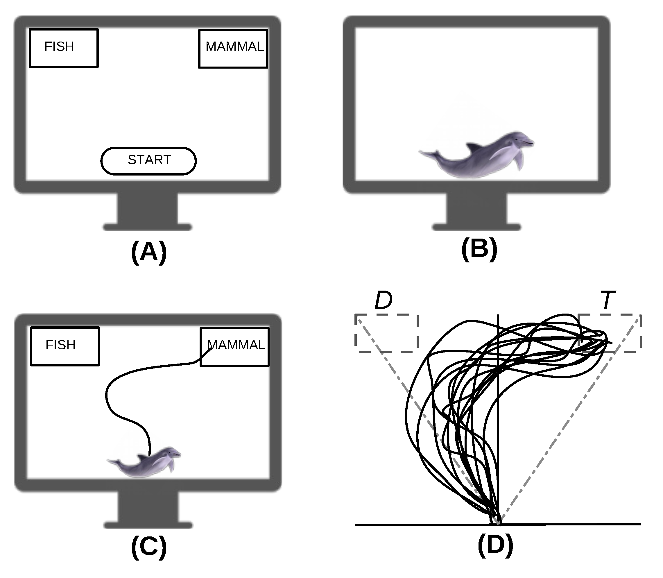
Figure 1. A typical mouse-tracking task: (A,B) Stimulus presentation, (C) participant’s response, (D) prototypical mouse-tracking trajectories for a set of participants and trials. Note that the correct response is presented on the top-right corner (T) whereas the corresponding competing response is presented on the top-left corner (D).
Mca 25 00041 g001
Figure 2. Simulated mouse-tracking trajectories Y plotted over time step n = 1 , , N . The data refer to a univariate design with I = 2 (rows of the plot), K = 2 (columns of the plot) and J = 6 (colors of the plot). Note that each of the K levels has J / K trials, T and D indicate Target and Distractor sections of the movement space.
Mca 25 00041 g002
Figure 3. language dataset: Mouse-tracking trajectories Y plotted over the time step n = 1 , , N . Note that the categorical levels are represented column-wise, subjects are represented row-wise, whereas distractor (D) and target (T) sections are represented above and below the solid gray line.
Mca 25 00041 g003
Figure 4. Illustrative example: MCMC traces, autocorrelation plots, and marginal posterior distributions for the model parameters. Note that all the Gelman-Rubin indices (Rhat) of the parameters are 1.0.
Mca 25 00041 g004
Figure 5. Illustrative example: Marginal posterior densities and violin plots for the levels of condition (recoded via dummy code). Note that black dots represent posterior means of the parameters γ whereas overlaps have been computed via the package overlapping [40].
Mca 25 00041 g005
Figure 6. Illustrative example: (A) Estimated latent dynamics X ^ for I = 5 subjects plotted over the scale N = 0 % , , 100 % . (B) log-Odd ratio for the evidence analysis.
Mca 25 00041 g006
Table 1. Overview of the contents of ssMousetrack.
FunctionTypeDescription
generate_data()mainsimulate data according to a user-defined experimental design.
run_ssm()mainrun state-space model on a given mouse-tracking dataset.
check_prior()mainallows users to define a list of priors for f ( γ ) prior running run_ssm().
prepare_data()mainpre-process raw tracking data prior running run_ssm().
evaluate_ssm()mainrun model evaluation given an output of run_ssm(). The function can plot results if requested by users.
compute_D()internalcompute the matrix of distances D given the observed data Y (see Equation (5)).
generate_Z()internalgenerate the Boolean trial-by-variable (design) matrix Z (see Equation (4)).
generate_design()internalallows users to specify an experimental design in terms individuals, trials, variables, and design matrix Z .
congruencydatasetsubset of data from Reference [4].
languagedatasetsubset of data from Reference [39].
Table 2. Illustrative example: Posterior quantities and Gelman-Rubin indices (Rhat) for the model parameters.
Meansd25%50%75%n_effRhat
gamma1 0.05 0.19 0.18 0.05 0.083047.001.00
gamma2 0.02 0.06 0.06 0.02 0.022764.001.00
gamma30.160.060.120.160.202782.001.00
gamma40.050.060.010.050.092680.001.00