Parallel Matrix-Free Higher-Order Finite Element Solvers for Phase-Field Fracture Problems

Abstract

Phase-field fracture models lead to variational problems that can be written as a coupled variational equality and inequality system. Numerically, such problems can be treated with Galerkin finite elements and primal-dual active set methods. Specifically, low-order and high-order finite elements may be employed, where, for the latter, only few studies exist to date. The most time-consuming part in the discrete version of the primal-dual active set (semi-smooth Newton) algorithm consists in the solutions of changing linear systems arising at each semi-smooth Newton step. We propose a new parallel matrix-free monolithic multigrid preconditioner for these systems. We provide two numerical tests, and discuss the performance of the parallel solver proposed in the paper. Furthermore, we compare our new preconditioner with a block-AMG preconditioner available in the literature.

1. Introduction

Many applications require the solution of partial differential equations (PDEs). Frequently, these are solved by Finite Element Methods (FEM), or related approaches like Isogeometric Analysis, which discretize the continuous PDE. To obtain accurate solutions, we eventually need to solve huge linear systems of equations. This may become a challenging task since the computational effort increases rapidly. Hence, solvers that are able to handle large-scale linear systems are required. This gives rise to specialized solvers, that are adapted towards a specific PDE. In this work, we focus on efficient parallel solvers for problems in phase-field fracture (PFF) propagation.

The origin of crack modeling dates back to Griffith [1] in 1921, who proposed the first model for fractures in brittle materials. The phase-field approach we are using was developed by Francfort and Marigo [2], who put the fracture model in an energy minimization context. Therein, the originally low-dimension crack is approximated by means of a continuous phase-field function. The PFF model was extended in [3,4,5] by decomposing the stress terms into tensile and compressive parts. However, the physically correct way to do this splitting is disputed within the fracture community. Examples exist where either one or the other method is superior. There has been developed a multitude of further extensions of the original model, e.g., to pressure-driven fractures [6,7,8] in porous-media [9,10,11,12], multi-physics [13] and many more; see also the survey papers [14,15,16] and the monograph [17].

PFF problems have the advantage that they reduce to a system of PDEs, which can be solved by adapting well-known strategies. On the other hand, a smooth approximation of an originally sharp fracture comes with some drawbacks, e.g., crack-length computation or interface boundary conditions along the fracture. There exist different approaches than PFF that allow treatment of sharp cracks, e.g., [18,19,20].

The numerical solution of PFF problems is particularly challenging, mainly due to the so-called no-heal condition. This ensures that a crack does not regenerate itself. Mathematically, this leads to an additional variational inequality. The solution gets further complicated by the non-convexity of the underlying energy functionals. Many different approaches have been proposed in the literature to handle PFF; see, e.g., [21,22,23,24,25]. In this work, we use the primal-dual active-set method, a version of the semi-smooth Newton method [26], which was applied to PFF in [24].

The most time consuming part in the simulation of PDEs is the solution of the arising linear systems of equations. In the context of nonlinear PDEs, these appear after linearization within Newton’s algorithm, or similar linearization approaches. Hence, multiple linear systems need to be solved per simulation step. For increasing problem sizes, this becomes a severe bottleneck, and well optimized solvers are required. In [27], we present a solver based on the matrix-free framework of the C++ FEM library deal.II [28]. Matrix-free methods avoid storing the huge linear system, which can become a real issue in terms of memory consumption. Further strategies treating the linear systems in phase-field fracture are presented in [24,29,30]. However, we notice that a competitive parallel linear solver was only presented in [30] to date. Therein, an algebraic multigrid (AMG) based solver with a block-diagonal preconditioner was employed. In regard to parallel matrix-free solutions, the closest work is the very recently published study [31] for finite-strain hyperelasticity. However, the implementation of the lastly mentioned solver to phase-field fracture (i.e., a nonlinear coupled problem with inequality constraints) is novel to the best of our knowledge.

To solve the linear systems, we use the iterative Generalized Minimum Residual (GMRES) method. Like many iterative solvers, this only requires matrix-vector multiplications, which can be carried out without assembling the matrix beforehand. To accelerate convergence, we employ a geometric multigrid (GMG) preconditioner with Chebyshev-Jacobi smoother. Again, all components of the GMG (level transfer, coarse operators, smoother) can be executed without explicit access to the matrix entries. For the Jacobi part, we additionally require the inverse diagonal of the matrix, which can be efficiently precomputed and stored also in the matrix-free context.

Matrix-free approaches are particularly favorable for high-polynomial degree shape-functions. In these cases, the number of non-zero entries per row within the sparse-matrix grows. This increases the storage cost per dof and also the computational effort of the sparse-matrix-vector multiplication (SpMV). On the other hand, matrix-free methods are less affected by higher polynomial degrees. These approaches originate from the field of spectral methods [32,33], where high-order ansatz functions are used.

The goal of this paper is a GMG preconditioned, matrix-free parallel primal-dual active-set method for nonlinear problems with inequality constraints, i.e., in our case, PFF. Moreover, we extend our previous work [27] to higher-order polynomial degrees. First, we are interested in the distributed solution of the whole problem. Therein, the computational work is split across multiple CPUs (ranks), each with its own independent memory. Necessary data exchange among CPUs is done using the Message Passing Interface (MPI). Using multiple CPUs gives us the possibility to fit larger problems into memory, as each core only stores small, almost independent parts of computational domain. All cores run in parallel, resulting in faster computations. Secondly, we explicitly utilize vector instruction sets provided by modern CPUs. These are special instructions for the CPU that are capable of performing multiple computations at once. This is more thoroughly described in Section 4.2.

In addition to the previously mentioned developments, we compare the performance of the AMG-based solver by [30] and the matrix-free geometric multigrid from our previous work [27]. Both approaches as well as the treatment of the nonlinearities are given in Section 3. In Section 6, we compare both approaches with respect to (wrt) computational time, memory consumption and parallel efficiency. Details on the parallelization are presented in Section 4. We focus on dependence on the polynomial degree of the finite elements. For studies regarding h-dependence, we refer to the respective papers. Section 5 describes the numerical examples and compares the results to those found in the literature to validate our implementations. Details on the phase-field model are briefly described in Section 2, for more information we refer to the corresponding literature. We also added a discussion on the derivative of the eigensystem in Section 3.5.

2. Preliminaries

In the following, we repeat the basic notation used in [27] as well as the governing equations. Furthermore, we introduce the primal-dual active-set method that can be interpreted as semi-smooth Newton method. Finally, we present the computation of the derivative of the eigensystem that plays a fundamental role in Miehe-type splittings.

2.1. Phase-Field Fracture Model

We use $(a,b):={(a,b)}_D:={\int }_{D}a·bdx$ for the standard $L^2$ scalar product, and $(A,B):={(A,B)}_D:={\int }_{D}A:Bdx$ for tensor-valued functions.

Figure 1 shows the computational domain $D\subset {\mathbb{R}}^d$ with an inscribed fracture $\mathcal{C}\subset {\mathbb{R}}^{d-1}$. The remaining undamaged parts of D are denoted by $\Omega$. We use the phase-field approach from [21,34,35], where the lower-dimensional fracture is approximated by using an additional scalar function $\phi :D\to [0,1]$. Values of 0 denote a completely fractured domain, whereas 1 represents undamaged parts. The size of the fracture approximation is controlled by the length-scale parameter $\epsilon$.

The unknown displacement field $u:D\to {\mathbb{R}}^d$ and fracture $\phi :D\to [0,1]$ are computed by means of an energy minimization problem

$$\mathcal{E}(u,\phi )={\int }_{D}g\left(\phi \right)E_s\left(e\right)dx+\frac{G_c}{2}(\frac{1}{\epsilon }{\parallel 1-\phi \parallel }^2+{\epsilon \parallel \nabla \phi \parallel }^2)\to min,$$

with additional displacement boundary conditions on $\partial D$.

The decay of the material stiffness is controlled by the degradation function $g\left(\phi \right)$. In this work, we use $g\left(\phi \right):=(1-\kappa ){\phi }^2+\kappa$, with a small positive regularization parameter $\kappa \ll 1$ to avoid singularities in fractured domains. Different choices of g can be found in the literature; see, e.g., [21,36,37,38].

The solid energy $E_s\left(e\right)$ is given by $\frac{1}{2}\lambda {\mathrm{tr}}^2\left(e\right)+\mu (e,e)$ with the strain tensor $e:=\frac{1}{2}(\nabla u+\nabla u^T)$ and Lamé parameters $\mu$ and $\lambda$.

We will further consider splitting the elastic energy into tensile and compressive parts $E_s=E_s^{+}+E_s^{-}$ based on the spectral decomposition proposed by Miehe and coworkers in [3]. The modified elastic energy functional then reads $E_s^{+}:=\frac{1}{2}\lambda {\langle \mathrm{tr}\left(e\right)\rangle }_{+}^2+\mu \mathrm{tr}\left(e_{+}^2\right)$, see [3,23]. Here, $a^{+}:=max(0,a)$ for real numbers a, and $e^{+}:={\sum }_{i=1}^d{\lambda }_i^{+}{v}_i\otimes v_i,$ for matrices e with eigensystem $({\lambda }_i,v_i)$.

Consequently, the stress tensor splitting is defined as ${\sigma }^{+}\left(u\right)={\partial }_e{E}_s^{+}$, i.e., ${\sigma }^{+}\left(e\left(u\right)\right)=\lambda \mathrm{tr}{\left(e\right)}^{+}I+2\mu e^{+}$. Various splitting schemes are discussed in [39] (Section 2.2) and [5].

This gives rise to the extended energy functional

$$\mathcal{E}(u,\phi )={\int }_{D}g\left(\phi \right)E_s^{+}\left(e\right)+E_s^{-}dx+\frac{G_c}{2}(\frac{1}{\epsilon }{\parallel 1-\phi \parallel }^2+{\epsilon \parallel \nabla \phi \parallel }^2)\to min,$$

Furthermore, fractures are only allowed to grow, i.e., ${\partial }_t\phi <0$. In our quasi-static formulation, this means that, for each loading step n, we need to enforce ${\phi }^n\le {\phi }^{n-1}$ almost everywhere (a.e.) in D. The first-order necessary condition (Euler–Lagrange system) of Section 2.1 is given by the following variational inequality problem

Problem 1.

(Euler–Lagrange System). Find displacement $u\in V$ and fracture $\phi \in W_{in}$ such that

$$\begin{array}{ccc}\hfill & \left(g\left(\phi \right){\sigma }^{+}\left(u\right),e\left(w\right)\right)+\left({\sigma }^{-}\left(u\right),e\left(w\right)\right)=0\hfill & \hfill \forall w\in V,\\ \hfill & \left({\partial }_{\phi }g\left(\phi \right)E_s^{+}\left(e\left(u\right)\right),\psi -\phi \right)\hfill \\ \hfill & +G_c\left(-\frac{1}{\epsilon }(1-\phi ,\psi -\phi )+\epsilon \left(\nabla \phi ,\nabla (\psi -\phi )\right)\right)\ge 0\hfill & \hfill \forall \psi \in W\cap L^{\infty }\left(D\right),\end{array}$$

with spaces $V:=H_0^1{\left(D\right)}^d,W:=H^1\left(D\right),W_{in}:=\{w\in W:w\le {\phi }^{old}a.e.inD\}$; see, e.g., [10].

Remark 1.

In the literature, the phase-field approximation described here is also referred to as AT 2 model (named after Ambrosio/Tortorelli) introduced in [34] for the Mumford–Shah problem and the original variational fracture formulation [21]. Changing the last line in Problem 1 leads to another well-known model referred to as AT 1; see, e.g., [40]. However, in this work, we only consider the AT 2 model.

2.2. Treatment of the Variational Inequality Constraints

Solving such variational inequalities is a challenging task that admits many different solution techniques. Popular choices are penalization approaches, where one incorporates violations to the no-heal condition into the variational form, i.e., adding terms like $\gamma {(\phi -{\phi }^{n-1})}^{+}$ for large enough values of $\gamma$. Improvements as in [22,41] aim to determine $\gamma$ adaptively, or provide lower bounds as in [38]. In [23], the inequality is replaced by a so-called history field $\mathcal{H}(x,t):=max\left\{E_s^{+}\left(e\left(u\right)\right)\right\}$, which again leads to an equality system to be solved.

In this work, we use the primal-dual active-set method for fractures as presented in [24]. In the next section, we continue with the description of the solution approaches used in our simulations, including details to the finite element version of the active-set algorithm mentioned above.

3. Discretization and Solution Algorithms

In this section, we briefly discuss the discretization methods used. We start with a very short description of FEM. More details can be found in one of the standard textbooks. We continue with the key parts of our solution strategy: the primal-dual active-set method and the linear solvers used therein. In Section 3.5, we illustrate how the derivative of the eigenvector and eigenvalues is computed in the case of Miehe-type splitting.

3.1. Finite Element Discretization

In particular, we use the Finite Element Methods on quadrilateral/hexahedral meshes to obtain discrete spaces for displacement and phase-field variables. The shape functions are chosen to be globally continuous piecewise polynomials of degree p in every coordinate direction ($Q_p$). The code is implemented in C++ with the help of the FEM library deal.II [28]. We make particular use of the matrix-free geometric multigrid framework included, which is described in more detail in [42,43].

3.2. Primal-Dual Active-Set Algorithm

The idea of the active-set algorithm is to enforce the constraints on a set $\mathcal{A}$, and perform a Newton step on the remaining dofs as outlined in Algorithm 1. The non-convexity of $\mathcal{E}$ leads to catastrophic convergence behavior of the active-set algorithm. To overcome this, we employ an extrapolation scheme as used in [24]. In the residual (1), this replaces the critical terms ${\phi }^2$ in the degradation function g by a prediction ${\tilde{\phi }}^2$, computed via linear extrapolation from the solutions of the previous two time-steps.

Algorithm 1 Primal-dual active-set.

Repeat for $k=0,\dots$ until ${\mathcal{A}}_k={\mathcal{A}}_{k-1}$ and $\parallel R_k\parallel \le {\epsilon }_{as}$:

1: Determine active-set ${\mathcal{A}}_k=\{i\mid {\left(M^{-1}{R}_k\right)}_i+c{(U_k-U^{old})}_i>0,\mathrm{for}\mathrm{phase}-\mathrm{field}\mathrm{dofs}i\}$ 2: Fix $\delta {\phi }_k=0\forall i\in \mathcal{A}$ 3: Newton-step $U_{k+1}=U_k+G_k^{-1}{R}_k$ on ${\mathcal{A}}_k^c$ 4: Check convergence

The nonlinear residual at the evaluation point $(u,\phi )\in V\times W_{in}$ is given by

$$\begin{array}{c}\hfill \begin{array}{cc}\hfill R(u,\phi )(w,\psi )& =\left(g\left(\tilde{\phi }\right){\sigma }^{+}\left(u\right),e\left(w\right)\right)+\left({\sigma }^{-}\left(u\right),e\left(w\right)\right)+\left({\partial }_{\phi }g\left(\phi \right)E_s^{+}\left(e\left(u\right)\right),\psi \right)\hfill \\ \hfill & +G_c\left(-\frac{1}{\epsilon }(1-\phi ,\psi )+\epsilon \left(\nabla \phi ,\nabla \psi \right)\right),\hfill \end{array}\end{array}$$

(1)

with test-functions $(w,\psi )\in V\times W$. Its derivative at $(u,\phi )$ in directions $\delta u$ and $\delta \phi$ equals to

$$\begin{array}{c}\hfill \begin{array}{cc}\hfill G(u,\phi )(w,\psi )(\delta u,\delta \phi )=& \left(g\left(\tilde{\phi }\right){\partial }_u{\sigma }^{+}\left(u\right)\left(\delta u\right),e\left(w\right)\right)+\left({\partial }_u{\sigma }^{-}\left(u\right)\left(\delta u\right),e\left(w\right)\right)\hfill \\ \hfill & +\left({\partial }_{\phi }g\left(\phi \right){\partial }_u\left(E_s^{+}\left(e\left(u\right)\right)\right)\left(\delta u\right),\psi \right)+\left({\partial }_{\phi \phi }^{2}g\left(\phi \right)E_s^{+}\left(e\left(u\right)\right)\delta \phi ,\psi \right)\hfill \\ \hfill & +G_c\left(\frac{1}{\epsilon }(\delta \phi ,\psi )+\epsilon (\nabla \delta \phi ,\nabla \psi )\right).\hfill \end{array}\end{array}$$

(2)

The partial derivatives wrt $\phi$ of the first term in R vanish since we have replaced $\phi$ by an extrapolation $\tilde{\phi }$. The corresponding discrete versions at the k-th step of Algorithm 1 are denoted by $R_k$ and $G_k$.

To evaluate $G(u,\phi )(w,\psi )(\delta u,\delta \phi )$, we need to compute the linearization of ${\sigma }^{+}$. This is challenging, as ${\sigma }^{+}$ is defined in terms of a spectral decomposition. In Section 3.5, we present an algorithm for the derivatives of the eigensystem. Computing the stress splitting is expensive, as seen in Section 6.3.

3.3. Linear Solvers

The crucial step in the solution of Problem 1 by the active-set method is the solution of the linear system $G_k·\delta U=R_k$ on ${\mathcal{A}}_k^c$. The system to be solved has the following block structure

$$\left(\begin{array}{cc}{G}_{uu}& 0\\ G_{\phi u}& G_{\phi \phi }.\end{array}\right)·\left(\begin{array}{c}\delta u\\ \delta \phi \end{array}\right)=\left(\begin{array}{c}{R}^u\\ R^{\phi }\end{array}\right).$$

A class of very powerful methods to solve linear systems arising from discretized PDEs are the multigrid methods. These aim to reduce and solve the problem on a hierarchy of nested spaces. Two frequently used types of multigrid solvers are the Algebraic Multigrid (AMG) and the Geometric Multigrid (GMG). Within the GMG approach, nested spaces are constructed by a hierarchy of meshes, i.e., it requires information about the geometry. On the other hand, AMG solvers work solely on the given sparse-matrix. There, hierarchies are extracted from the (weighted) connectivity graph of the matrix, see, e.g., [44]. Since AMG only needs the linear system to be solved as an input, they are often considered to be black-box solvers. This is, however, a huge oversimplification, as there are many different AMG methods and options tailored to specific classes of PDEs. For more details on AMG, GMG and multigrid in general, we refer to [44,45,46,47,48].

To solve these equations, we use two different approaches. First, we use the matrix-free multigrid framework from deal.II extended to handle nonlinear variational inequalities arising from PFF, see [27], and also [31] for a very recent work on the matrix-free solution of nonlinear hyperelastic problems. This uses a monolithic geometric multigrid for the whole system. The special structure of the matrix is utilized inside the smoother, i.e., we use

$$P_{GMG}^{-1}:=GMG\left(G\right)\mathrm{with}\mathrm{block-diagonal}\mathrm{smoother}\mathcal{S}:=\left(\begin{array}{cc}S\left(G_{uu}\right)& 0\\ 0& S\left(G_{\phi \phi }\right)\end{array}\right),$$

and Chebyshev–Jacobi smoothers S acting on the single blocks. These smoothers are frequently used in the context of matrix-free methods. Contrary to standard smoothers like Gauss–Seidel, Chebyshev–Jacobi smoothers only require matrix-vector multiplications and scaling with the diagonal. Both operations can be done in a matrix-free fashion, which we will describe later on. We continue with a brief description of the Chebyshev smoother. For more details we refer to the literature, see, e.g., [49], or [50,51] in the context of HPC. Chebyshev-type methods work on a given eigenvalue spectrum $[a,b]$. Depending on the choice of this interval, we can use the Chebyshev method as smoother but also as a solver. A solver should handle the whole spectrum of the operator. Hence, we want to have $a\le {\lambda }_{min}<{\lambda }_{max}\le b$ with the extremal eigenvalues ${\lambda }_{min}$ and ${\lambda }_{max}$ of $G_{uu}$ resp. $G_{\phi \phi }$. This is required on the coarsest grid of the multigrid algorithm, where we want to solve the system more accurately. The main intention of the Chebyshev–Jacobi method, however, is smoothing. Here, we are not interested in treating the whole spectrum, but only the high-frequency parts. A choice of $[a,b]:=[c{\lambda }_{max},C{\lambda }_{max}]$ with $c\le 1$ and $C\ge 1$ is frequently used. In our applications, we use $c=0.24$ and $C=1.2$. This involves knowledge about ${\lambda }_{max}$ (and also ${\lambda }_{min}$ for the solving part). For symmetric positive definite matrices, CG can be used to obtain an estimate of both eigenvalues. Within PFF, symmetry of $G_{uu}$ and $G_{\phi \phi }$ follows from the second derivative of the energy functional. We could not rigorously show positive definiteness for these blocks, but numerical studies did not give us contradicting results.

In a second approach, we compare our MF-GMG preconditioner to the block-diagonal AMG preconditioner presented in [30]. The linear system is then preconditioned by

$$P_{AMG}^{-1}:=\left(\begin{array}{cc}AMG\left(G_{uu}\right)& 0\\ 0& AMG\left(G_{\phi \phi }\right)\end{array}\right),$$

with Trilinos/MueLu AMG [52,53] solvers for the diagonal blocks. In both cases, we use GMRES as outer solver and use $P_{AMG}^{-1}$ resp. $GMG\left(G\right)$ as preconditioners.

3.4. Matrix-Free Representation

The main idea of matrix-free approaches is to avoid assembling and storing sparse (but huge) matrices. This is reasonable since iterative solvers like Conjugate Gradients (CG) or Generalized Minimal Residual (GMRES) do not require explicit knowledge about the entries of the matrix. Rather, these solvers only need the result of the matrix-vector multiplication (MV). We combine the assembly and sparse matrix-vector multiplication (SpMV) by

$$G·\delta U=\sum _{k=1}^{n_e}{C}^T{P}_k^T{G}_k\left(P_{k}C\delta U\right),$$

with the number of elements $n_e$, possible constraints C, element-wise global-to-local mapping $P_k$ and the local stiffness matrices $G_k$ corresponding to (2). This is already a valid matrix-free matrix-vector product (MFMV). However, its computational complexity of $\mathcal{O}\left(p^{2d}\right)$ per element matches those of the classical SpMV. Hence, we cannot expect to gain performance compared to the usage of an assembled sparse-matrix; further optimizations are needed. These are thoroughly described in [54,55], and already included in the matrix-free classes of the deal.II library. The key point is to apply sum-factorization techniques in the computation of $G_k$. This exploits the tensor-product structure of the shape-functions and quadrature points on the reference element ${[0,1]}^d$. Eventually, this reduces the complexity to $\mathcal{O}\left(p^{d+1}\right)$. Hence we expect the matrix-free version to outperform the SpMV for high-polynomial degrees, in particular in $3d$, which is indeed verified in Section 6.3.

3.5. Derivatives of the Eigensystem

In the case of Miehe-type splittings of the stress tensor, we require the derivatives of ${\sigma }^{+}$ and ${\sigma }^{-}$ in direction $\delta u$, which depend on the eigensystem of the strain tensor. In the following, we illustrate how to compute these quantities for arbitrary (but small) dimensions. The following derivation holds for real symmetric matrices, and in particular for the solid strain tensor.

We assume, that the matrix A and $\delta A$, as well as the eigenvector and eigenvalue of A, denoted by $\lambda$ and v, are available such that

$$Av=\lambda v,\mathrm{with}\parallel v\parallel =1,$$

(3)

holds. In our application, the direction $\delta A$ is given in terms of the displacement test functions. The eigensystem of A itself can easily be computed explicitly in $2d$ and $3d$, e.g., with the help of some computer algebra system. For higher dimensions, more sophisticated methods are available. Taking the derivative of (3), we get by the product rule

$$\delta A·v+A·\delta v=\delta \lambda v+\lambda \delta v.$$

(4)

Forming the ${\ell }_2$-scalar-product of (4) with v yields

$$\left(\delta A·v,v\right)+\left(A·\delta v,v\right)=\left(\delta \lambda v,v\right)+\left(\lambda \delta v,v\right).$$

Using the symmetry of A and the normalization $\left(v,v\right)=1$, we can reduce it to

$$\left(\delta A·v,v\right)=\delta \lambda .$$

(5)

Since $\delta A$ and v are given, we can now compute the derivative of $\lambda$ by the formula above.

Computing the derivative of the eigenvector v is slightly more involved. We start by collecting the terms $\delta v$ in (4):

$$(A-\lambda I)·\delta v=\delta \lambda v-\delta A·v.$$

(6)

Unfortunately, we cannot simply invert $(A-\lambda I)=:L$ to obtain $\delta v$ since $\lambda$ is an eigenvalue of A. Hence, L is singular by definition. This is seen easily from (3), which can be rearranged to $L·v=0$. Therefore, we need the concept of a pseudo-inverse (or left-inverse), see, e.g., [56]. The pseudo-inverse $L^{†}$ has the properties (among others) that $L^{†}L=I$ and $L^{†}w=0\forall w\in \mathcal{N}\left(L\right)=span\left\{v\right\}$. Utilizing this, we can apply $L^{†}$ to (6), and get

$$L^{†}L·\delta v=L^{†}\delta \lambda v-L^{†}\delta A·v,$$

which finally reduces to

$$\delta v=-L^{†}\delta A·v.$$

(7)

With (5) and (7) we can now compute the linearized eigensystem of A.

If the eigensystem $({\lambda }_i,v_i)$ of A is known, we can decompose $A=VD{V}^T$ with the matrix of eigenvectors $V=(v_1,\dots ,v_d)$ and diagonal matrix $D=\mathrm{diag}({\lambda }_1,\dots ,{\lambda }_d)$. Furthermore, we have $L=V(D-\lambda I)V^T$. Then, the pseudo-inverse can be computed as

$$L^{†}=V{D}^{†}{V}^T,$$

with $D^{†}:=\left\{\begin{array}{cc}0\hfill & \mathrm{if}{\lambda }_i-\lambda =0\hfill \\ \frac{1}{{\lambda }_i-\lambda }\hfill & \mathrm{if}{\lambda }_i-\lambda \ne 0.\hfill \end{array}\right.$

This machinery can be applied to compute $e^{+}$ and its derivative for arbitrary dimensions, see Algorithm 2 for the detailed steps. The derivative of ${\sigma }^{+}\left(e\right)$ follows by

$${\partial }_u{\sigma }^{+}\left(u\right)\left(du\right)=\lambda \left\{\begin{array}{c}\hfill \begin{array}{cc}0\hfill & \mathrm{if}\mathrm{tr}\left(e\right(u\left)\right)<0\\ \hfill \mathrm{tr}\left(e\right(du\left)\right)& \mathrm{else}\hfill \end{array}\end{array}\right\}I+2\mu {\partial }_e\left(e^{+}\right)\left(e\left(du\right)\right).$$

Algorithm 2

1: Input:$A,\delta A\in {\mathbb{R}}^{d\times d},d=2,3$ 2: Output:${\partial }_A{A}^{+}\left(A\right)\left(\delta A\right)\in {\mathbb{R}}^{d\times d}$            ▹ Derivative of $A^{+}$ at A in direction $\delta A$ 3:   4: Decompose $A=VD{V}^T$ 5:   6: for$i\in \{1,\dots ,d\}$do 7:  $L=A-{\lambda }_{i}I$ 8:  $D^{†}:=\mathrm{diag}(\frac{1}{{\lambda }_1-{\lambda }_i},\dots ,\frac{1}{{\lambda }_d-{\lambda }_i})$ 9:  $L^{†}=V{D}^{†}{V}^T$ 10:  $d{v}_i=-L^{†}\delta A·v_i$ 11:  $d{\lambda }_i=v_i^T\delta A{v}_i$ 12:  $d{\lambda }_i^{+}=\left\{\begin{array}{cc}0\hfill & \mathrm{if}{\lambda }_i<0\hfill \\ d{\lambda }_i\hfill & \mathrm{if}{\lambda }_i\ge 0\end{array}\right.$ 13: end for 14:   15: $\delta V=(d{v}_1,\dots ,d{v}_d)$ 16: $\delta D^{+}=\mathrm{diag}(\delta {\lambda }_1^{+},\dots ,\delta {\lambda }_d^{+})$ 17:   18: $A^{+}:=V{D}^{+}{V}^T$ 19:   20: return$\partial A^{+}\left(A\right)\left(\delta A\right):=\delta V{D}^{+}{V}^T+V\delta D^{+}{V}^T+V{D}^{+}\delta V^T$

4. Parallel Implementation

The finite element library deal.II as well as our implementation are parallelized on multiple levels. First of all, the problem is split across multiple CPUs such that each of them only stores and handles a small subset of the whole problem (distributed parallelization). Necessary communication between different CPUs is handled via the message passing interface (MPI). Furthermore, each CPU runs explicitly vectorized code, that is, multiple data elements are handled with the same CPU instruction. The next subsections explain these concepts in more detail.

4.1. Distributed Parallelization

When dealing with large problems, it may no longer be possible for a single CPU to store all the required infrastructure in memory. Hence, the computational problem is split into smaller chunks which are distributed among multiple CPUs. In the context of FEM, this is typically done by assigning each CPU some parts of the mesh. Such a partitioning can be achieved by using libraries like p4est [57]. Each CPU then handles all the dofs associated to its part of the mesh (owned dofs). Furthermore, it may occasionally require knowledge about additional dofs which are owned by another CPU (ghost dofs), e.g., if we want to evaluate solutions close to the interface between different CPUs. These information needs to be shared among multiple CPUs, which is done via the message passing interface (MPI). This provides methods for communication in distributed networks. deal.II provides an easy to use infrastructure for these kind of tasks; see, e.g., [58].

4.2. Vectorization

Within the matrix-free framework, deal.II makes use of the CPU vector instruction set. These operations perform single instructions on multiple data (SIMD). In the following, we illustrate the most basic idea of SIMD. Further details can be found in the respective literature, see, e.g., [59]. Consider the simple implementation of adding two vectors: $r\left[i\right]=a\left[i\right]+b\left[i\right]i=0,\dots 3$. This would take the CPU to issue one add instruction per vector entry, i.e., a total of four instructions (ignoring CPU instructions required for the loop, assignment, etc.). However, modern CPUs are capable of performing the same operations on multiple elements at once. Hence, only one add instruction is required for the simple example above, resulting in a hypothetical speedup of 4. Depending on the CPU, different vectorization sizes are possible. The most recent CPUs support 128 bit, 256 bit and 512 bit instructions. Hence, $2,4$ and 8 double precision values or $4,8$ and 16 single precision values may be treated simultaneously.

There are several important points to consider here. First of all, vectorization requires the same work to be done on all entries. Hence, code with branching, e.g., if statements with a condition depending on the values cannot be efficiently vectorized. Workarounds usually involve executing both branches for each vector element and merging them via bit masks, see Algorithm 3. These type of instructions are called “blend”. This is mainly used for simple if-then-else assignments, i.e., $x\left[i\right]=\left\{\begin{array}{cc}a\left[i\right]\hfill & \mathrm{if}a\left[i\right]>b\left[i\right]\hfill \\ 0\hfill & \mathrm{else}\hfill \end{array}\right.$, where the additional overhead of executing all branches and combining the results does not dominate the benefits of using vectorized code.

Algorithm 3 Vectorized if-then-else statement using bit masks.

1: Input: $a,b\in {\mathbb{R}}^v$, $v=1,2,4,$ or 8 2: Output: $x\left[i\right]=\left\{\begin{array}{cc}a\left[i\right]\hfill & \mathrm{if}a\left[i\right]>b\left[i\right]\hfill \\ 0\hfill & \mathrm{else}\hfill \end{array}\right.$ 3: $mask=x<y$   ▹ a bitmask, with all bits of element i set to 1 if $x\left[i\right]<y\left[i\right]$, and or 0 otherwise 4: $a0=a$ & mask       ▹ bitwise ’and’ operation. Each entry equals to either the entry of a or 0 5: $b0=b$ & !mask      ▹ similar to above: each entry is either part of b (condition was false) or 0 6: $result=a0|b0$            ▹ combine the two branches by a bitwise ’or’ operation

An additional drawback of vectorization is the difficulty of implementation and portability. For simple algorithms, up-to-date compilers can automatically vectorize the loop. Unfortunately, this auto-vectorization ceases to work for more complex scenarios. This leaves the developer to explicitly call SIMD instructions of the form _mm512_add_pd, which makes the implementation more tedious. Usually, wrapper libraries are used to improve code readability and portability. For instance, the VectorizedArray class in deal.II or Vc [60] among others. Recently, there has also been effort to include vectorization capabilities into the C++ standard.

Within the deal.II matrix-free implementation, vectorization is done over elements. That is, each CPU instruction acts on multiple elements at once. Several implementational details are described in [54,55,61].

We now investigate the influence of different vectorization levels and compiler settings on the performance of the MFMV. All of these tests are carried out on a single core, using the single-edge notched shear test described in Section 5.2. We used $Q_1$ elements on a 6-times refined grid, but the observed speedup is valid also for different settings, as long as the problem size is not too small. Compilation was done using GCC-9.2.0 and clang-11.0.0 with flags -O3, -fma, -march=native, -mavx, -f(no)-tree-vectorize and -f(no)slp-vectorize (clang only). The test ran on an Intel Haswell Xeon E5-2630v3 with $2.4$ GHz clock speed, supporting vector instructions up to 256 bit, resp. 4 doubles. All computations were carried out using double precision floating point numbers. The average run time out of 100 is reported.

Our findings are summarized in

Table 1. Effect of vectorization within the matrix-free operator evaluation. Baseline is given by a standard release build using the $O3$ optimization flag without vectorization. (a) gcc, (b) clang.

(a)
Arguments	Speed-Up	Time (avg)
$O3$	1.00	$2.63\times {10}^{-2}$
$O3$, auto	1.02	$2.58\times {10}^{-2}$
128 bits,	2.00	$1.31\times {10}^{-2}$
128 bits, auto	2.04	$1.28\times {10}^{-2}$
256 bits,	2.29	$1.15\times {10}^{-2}$
256 bits, auto	2.28	$1.15\times {10}^{-2}$
(b)
Arguments	Speed-Up	Time (avg)
$O3$	1.00	$1.77\times {10}^{-2}$
$O3$, auto	1.00	$1.76\times {10}^{-2}$
128 bits,	1.69	$1.05\times {10}^{-2}$
128 bits, auto	1.69	$1.05\times {10}^{-2}$
256 bits,	2.54	$6.97\times {10}^{-3}$
256 bits, auto	2.63	$6.73\times {10}^{-3}$

for gcc (left) and clang (right). There, “auto” is used to denote enabled auto-vectorization. n-bits denotes explicit vectorization using the given number of bits, i.e., 128 for SSE and 256 for the AVX instruction set.

We notice that auto-vectorization does not give much speed-up for gcc. Explicit vectorization over elements doubles the performance, hence, yielding the best possible speedup using the 128 bit instruction set. Using 256 bit SIMD instructions only improved the results by another $25\%$. Possible explanations are the automatic throttling of the CPU speed [62] or memory bandwidth restrictions, but the actual reasons are unclear.

For clang, the SIMD behavior is vastly different. Again, auto-vectorization does not increase the performance in the O3 and 128 bit case. However, it adds another 9% speed-up for the 256 bit case. Furthermore, clang does not give near as good speed-up when using 128 bit instructions, but makes up for that when using AVX. Surprisingly, clang outperforms gcc by roughly a factor of $1.6$ in our simulation.

5. Numerical Examples

In the upcoming subsections, we present our numerical examples. We focus on a pair of well-known test cases for fracture propagation: the single-edge-notched shear and tension test. These have been well studied in the literature, such that we can compare our findings to those reported by other groups. Results regarding the performance of our solvers and their behavior under p-refinement follows in Section 6.

5.1. Example 1: Single-Edge Notched Tension Test

We start with the single-edge notched tension test. This test case has been studied by other groups as well, see, e.g., [3,5,23,24,63].

5.1.1. Description

The domain of interest is a unit square with a thin slit as shown in Figure 2. Due to the discontinuity in the geometry, we have two sets of dofs along the slit at the same locations. This is indicated by the double dot at $(0,0.5)$. Fracture propagation is driven by an increasing displacement pulling at the top boundary, i.e., $u=(0,t·du)\mathrm{on}{\Gamma }_{top}$. The specimen is fixed at the bottom by imposing $u=(0,0)\mathrm{on}{\Gamma }_{bottom}$.

Remark 2.

Due to symmetry, it would be sufficient to fix the y-component of u at ${\Gamma }_{bottom}$ and ${\Gamma }_{top}$ for the tension test. This yields the same results as using the boundary conditions specified above.

The material parameters for the tension test are shown in

Table 2. Material parameters and configuration for the single-edge notched shear/tension test cases.

Parameter	$\mathit{\lambda }$	$\mathit{\mu }$	${\mathit{G}}_{\mathit{c}}$	$\mathit{\kappa }$	$\mathit{dt}$	$\mathit{du}$
Value	$121.15$	$80.77$	$2.7\times {10}^{-3}$	${10}^{-10}$	1	${10}^{-5}$
Unit	kN/mm${}^2$	kN/mm${}^2$	kN/mm		s	mm

. All computations were done using $Q_1$-elements for displacement and phase-field on uniform quadrilateral grids.

Table 3. Values and parameters for the different refinement levels of the single-edge notched shear/tension tests.

ℓ	Dofs	Elements	h	$\mathit{\epsilon }$
6	$1.3\times {10}^4$	$4.1\times {10}^3$	$2.2\times {10}^{-2}$	$4\times {10}^{-3}$
7	$5.0\times {10}^4$	$1.6\times {10}^4$	$1.1\times {10}^{-2}$	$4\times {10}^{-3}$
8	$2.0\times {10}^5$	$6.6\times {10}^4$	$5.5\times {10}^{-3}$	$4\times {10}^{-3}$
9	$7.9\times {10}^5$	$2.6\times {10}^5$	$2.8\times {10}^{-3}$	$4\times {10}^{-3}$
10	$3.2\times {10}^6$	$1.0\times {10}^6$	$1.4\times {10}^{-3}$	$4\times {10}^{-3}$
11	$1.3\times {10}^7$	$4.2\times {10}^6$	$6.9\times {10}^{-4}$	$4\times {10}^{-3}$
12	$5.0\times {10}^7$	$1.7\times {10}^7$	$3.5\times {10}^{-4}$	$4\times {10}^{-3}$

lists the number of elements and dofs for each level of refinement ℓ.

5.1.2. Discussion

First, we perform a refinement study for the single-edge notched tension test. To this end, we fix all parameters and perform global mesh refinement. In particular, the phase-field parameter is fixed to $\epsilon =4\times {10}^{-3}$ as used in [5].

The resulting load-displacement curves are shown in Figure 3 for the anisotropic case (Miehe splitting). Whereas the solutions on the coarse meshes deviate a lot, the solutions on the fine meshes are almost indistinguishable showing the convergence of our implementation. In particular, the deviation to the solution on the finest mesh seems to decrease approximately by a factor of $0.5$ in every refinement step. The splitting does not seem to have much impact on this simulation. Indeed, the isotropic results agree almost perfectly with the anisotropic findings.

In comparison to the results presented in [5], the resulting maximum load is slightly higher in our computations. Furthermore, the decay of the loading force seems to take longer, i.e., the amount of displacement when the load hits zero is roughly $7\times {10}^{-3}$ in our case, whereas it is slightly less than $6\times {10}^{-3}$ in [5]. According to the findings in [5] (Figure 11), this zero-load point seems to be very sensitive to the selected time-step size, as well as the number of staggered iterations in their solution approach. We also notice that in [5] only a single mesh is considered, whereas we did convergence studies on seven refinement levels, which clearly show computational convergence.

5.2. Example 2: Single-Edge Notched Shear Test

The following test scenario is closely related to the previous tension test. Both have the same geometry and material parameters, but the boundary conditions are flipped.

5.2.1. Description

The computational domain is again given by a unit square, with the same slit imposed as in the previous test case. In this scenario, however, the applied displacement conditions moves from the top boundary to the right, i.e., $u=(t·du)\mathrm{on}{\Gamma }_{top}$. Again, the body remains fixed at the bottom by $u=(0,0)\mathrm{on}{\Gamma }_{bottom}$.

5.2.2. Discussion

In the isotropic case of the single-edge notched shear test in Figure 4, the load-displacement curves do not coincide with the observations in [5] but look more similar to their results with Amor-splitting. However, the observed crack pattern is similar, i.e., two symmetric branches appear as seen in Figure 5 (right). We like to point out that neither the Miehe-splitting nor the isotropic model lead to physically sound results, see, e.g., [5] and also the early work [3]. Nonetheless, one clearly observes mesh convergence as in the tension test.

Contrary to the tension test before, the resulting load-displacement curves show lots of small oscillations. This is partly also observed in [5], although the oscillations there are seemingly smaller. The results with Miehe splitting seem to match better, but the maximum load and displacement are lower than those reported by [5].

Figure 6 shows the test results for different polynomial degrees p. In the left plot, the refinement level corresponds to $\ell =7$, all other parameters are the same as before. The right plot varies both the polynomial degree and the refinement level, yielding $790k$ dofs in all cases. We immediately notice, that the small oscillations are gone for the high-order simulations. Furthermore, we also see convergence with respect to p. The number of dofs for degree p can be obtained from

Table 4. Dof counts for varying p for the single-edge notched shear/tension tests. (a) Mesh-refinement level $\ell =7$ and (b) $\ell =9$.

(a)
ℓ	p	dofs
7	1	$5.0\times {10}^4$
7	2	$2.0\times {10}^5$
7	3	$4.5\times {10}^5$
7	4	$7.9\times {10}^5$
(b)
ℓ	p	dofs
9	1	$7.9\times {10}^5$
9	2	$3.2\times {10}^6$
9	3	$7.1\times {10}^6$
9	4	$1.3\times {10}^7$

.

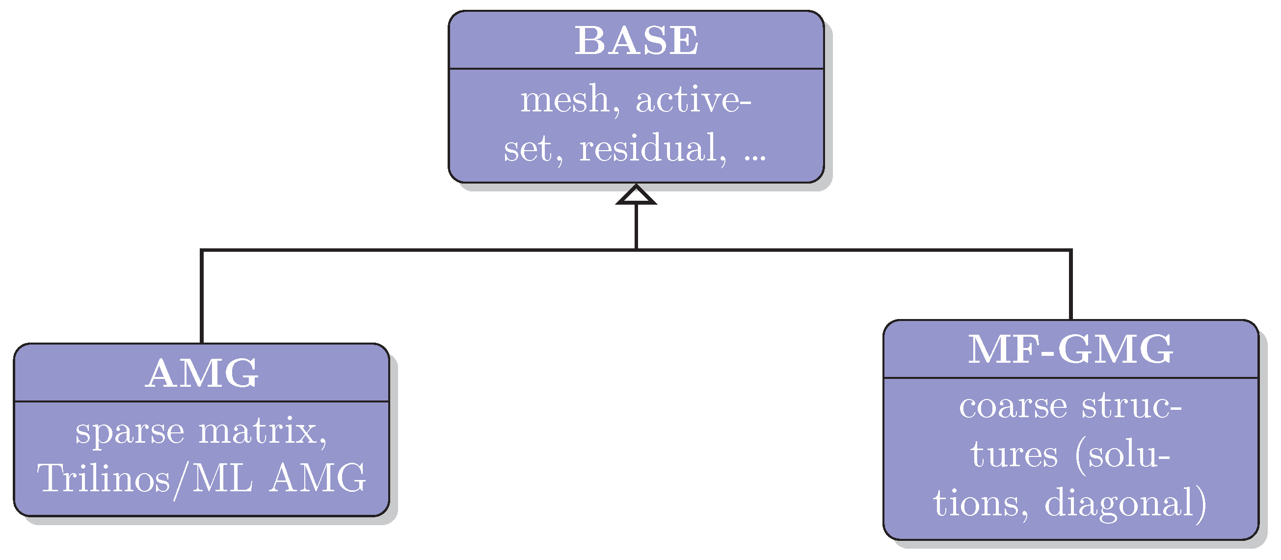
6. Performance Studies

In the upcoming subsections, we compare our matrix-free version with the AMG based preconditioner described in [30] in terms of iteration counts, memory requirements, computational time and scalability. We would like to point out that most of the code is shared between the two implementations, i.e., only the parts related to handle the linear system differ, as visualized in Figure 7. This allows for a fair comparison of the results.

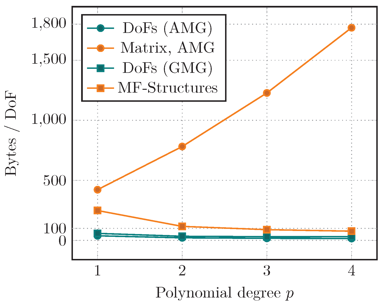
6.1. Memory Requirements

We start by investigating the memory requirements of the two approaches, which should be an obvious advantage of the matrix-free framework. Due to the required multigrid dofs for the geometric multigrid, the dof structures require slightly more memory compared to the AMG version. This is more than compensated by larger storage requirements of the sparse matrix and AMG hierarchies compared to the multilevel matrix-free structures in the GMG implementation. In particular for high-order polynomial degrees p, the sparse matrix gets increasingly dense, leading to huge memory costs. In fact, the number of non-zero entries per row (dof) increases as $\mathcal{O}\left(p^d\right)$. Unlike that, the cost for a dof within the matrix-free approach is almost independent of p.

All these effects are shown in Figure 8 for varying polynomial degree p. There, the average storage requirements per dof are visualized for several quantities:

• DoFs (AMG): handling of dofs on the fine level;
• Matrix, AMG: both the sparse-matrix and the AMG preconditioner;
• DoFs (GMG): handling of dofs including multigrid levels;
• MF-Structures: all necessary matrix-free and GMG structures.

Estimates on memory consumption are provided by objects from deal.II, as well as the AMG solver by ML. For a degree of 4, we save approximately a factor of 20 in terms of memory. These results are shown for a 2d test case. In 3d, this gap would even be more prominent.

6.2. Iteration Counts

Next, we have a look at the number of iterations required to solve the arising linear systems of equations. We would like to point out that these counts are highly dependent on the actual settings used, i.e., which simulation is run, selected number of smoothing steps, coarse level and further parameters. For the AMG solver, we use the Trilinos package ML [64], with Chebyshev–Jacobi smoother of degree 2, an aggregation threshold of $0.02$, damping $1.33$ and maximum coarse problem size of 2000. The GMG uses $\ell =2$ as coarse grid, i.e., 16 elements, and five Chebyshev–Jacobi smoothing sweeps. Increasing the number of smoothing steps would decrease the number of iterations. Finding a good balance between smoothing quality and iteration count to obtain the best performance is a very challenging task, which we did not consider in detail by now. In all our simulations, we use relative convergence criteria of ${10}^{-6}$ for the linear solver and ${10}^{-8}$ for the active-set strategy.

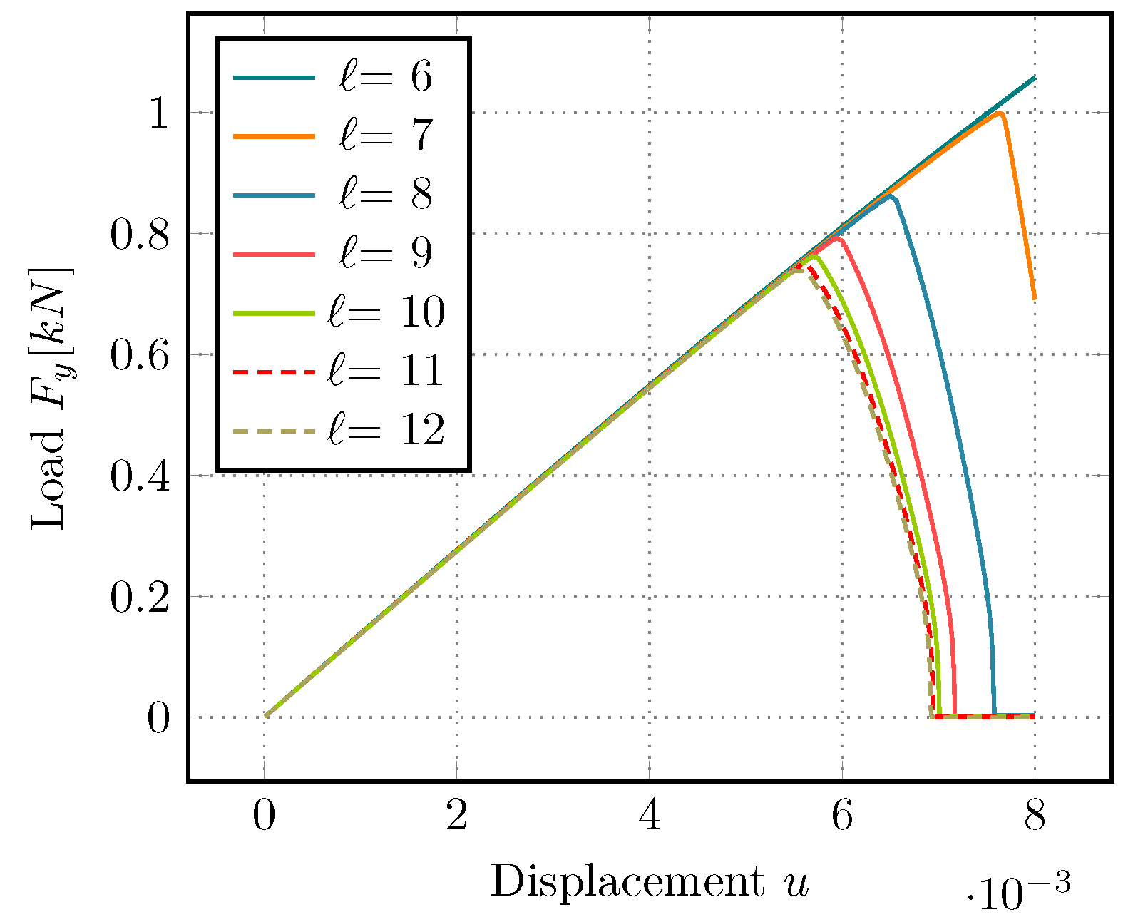
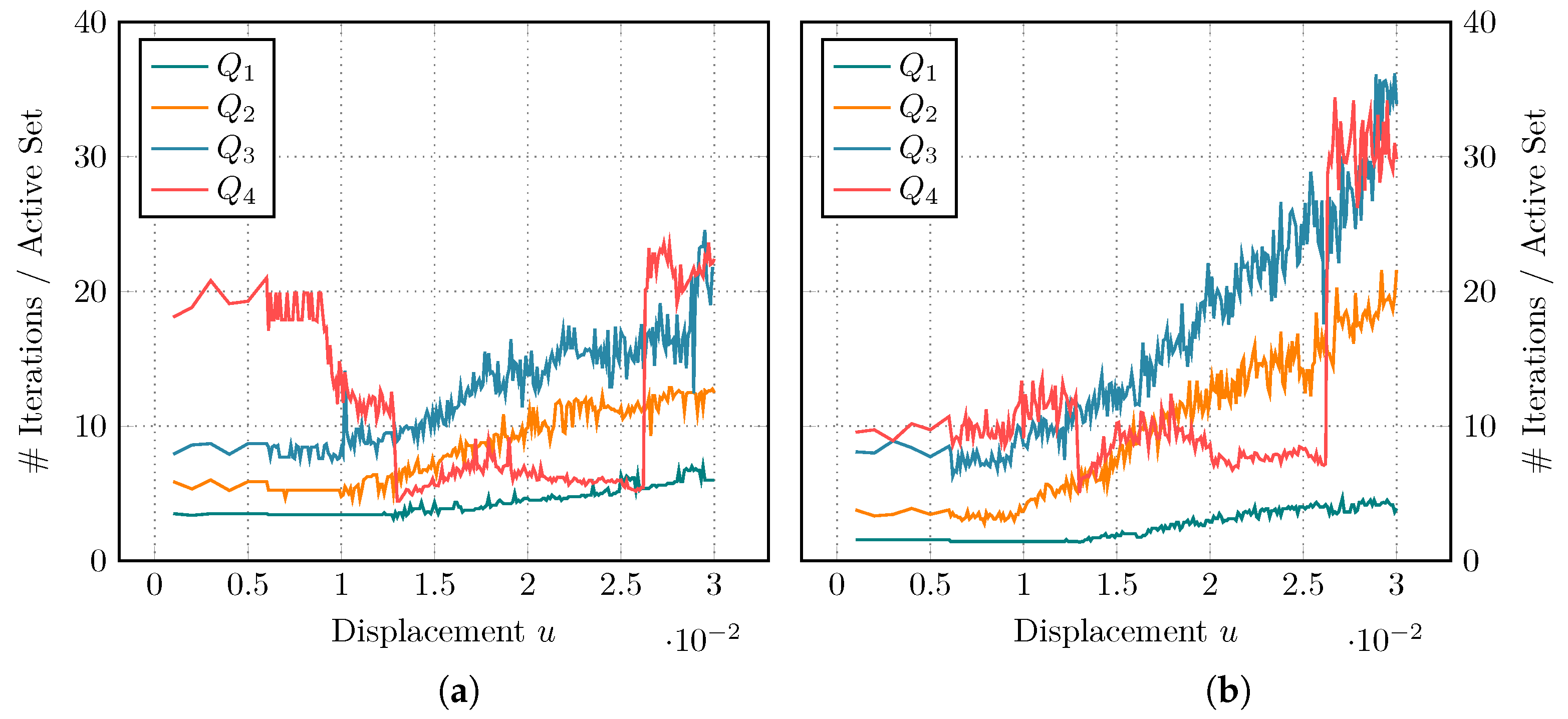
A representative comparison of the iteration behavior is given in Figure 9, with AMG results on the left and GMG results on the right side. Again, we vary the polynomial degree for the shear test, as this scenario shows more interesting behavior. Both approaches show an expected growth in the number of iterations for increasing p. We also observe that both solvers require more work as the fracture grows. Degree $p=4$ behaves somewhat surprisingly. It requires less steps in the middle of the simulation for both the AMG and GMG strategy. The iteration count jumps up towards the end of the simulation, when the domain is close to total failure.

6.3. Performance Analysis

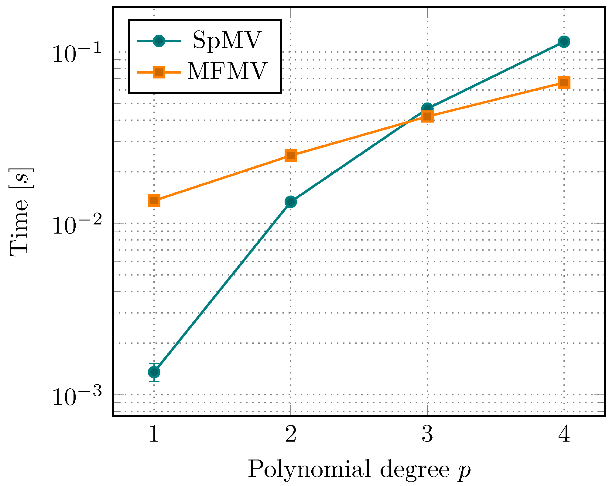
We continue to investigate the computational performance of the matrix-free approach. To this end, we start by comparing the sparse-matrix vector multiplication (SpMV) time with the corresponding matrix-free evaluation (MFMV). In Section 3.4, we learned that MFMV should be faster given high enough polynomial degrees. For all tests, we use explicit vectorization based on AVX-256 in the matrix-free parts as described in Section 4.2.

In [27], we compared the behavior with respect to h-refinement. Here, we want to focus on the dependence on the polynomial degree p. In Figure 10, we observe that SpMV is faster for linear and quadratic elements. However, this only considers the raw matrix-vector multiplication. In particular, it does not include the time that is required to assemble the matrix. We also notice, that starting from degree 3, MFMV starts to outperform SpMV even for single evaluations.

The results shown here are using the Miehe-type splitting, which is computationally expensive due to its dependence on the eigensystem. Compared to the isotropic model (no splitting), the performance of the MFMV drops by roughly 20–25% (2d) and 30–35% (3d). The assembly of the sparse-matrix is affected by approximately 7–10% in 2d, and 70% in 3d. A hybrid approach has been presented in [5] in order to overcome the high cost of the Miehe splitting. To speed-up the MFMV, approximations to $\partial {\sigma }^{+}$ could be a viable option, in particular if combined with caching of certain quantities as done in [31]. However, we did not consider this so far.

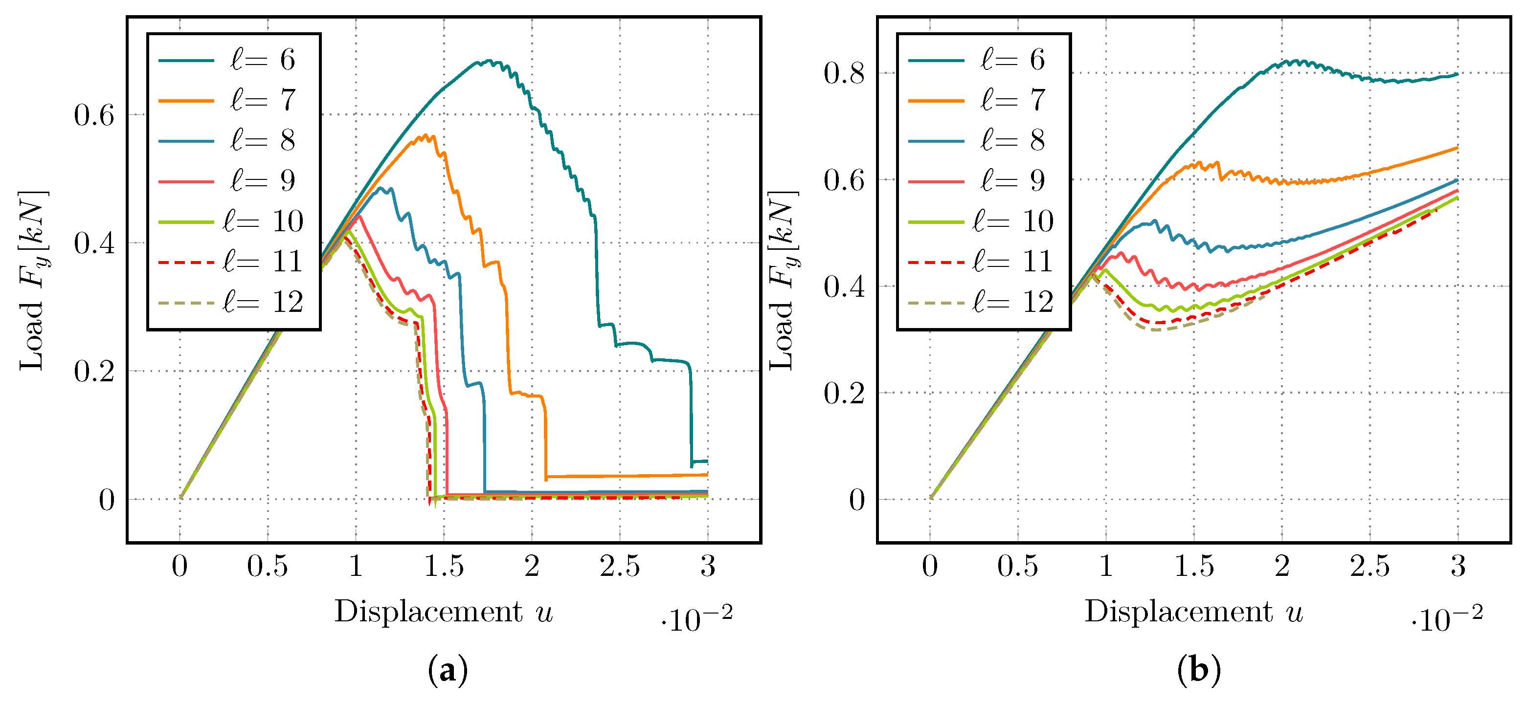
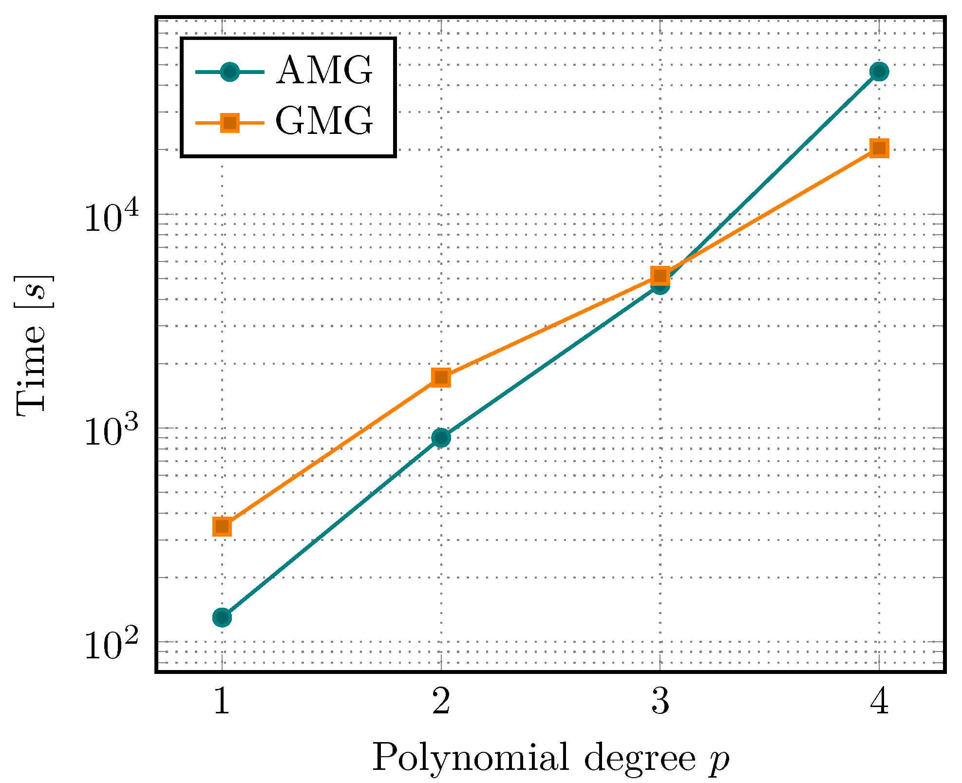
Let us now look at the performance of a full simulation. This is visualized in Figure 11, where the total time spent in the linear solvers, i.e., GMRES with either AMG or GMG as preconditioners, is plotted. Here, only a single simulation of the single-edged notched shear test is performed. Possible fluctuations in the timings should be evened out over the length of the simulation.

The observed behavior is very similar to the vmult-times presented before. The faster SpMV for linear and quadratic elements is able to overcome the time of assembling the matrix and initializing the AMG solver, thus ending up faster than the matrix-free solver. The situation shifts in favor of the MF-GMG preconditioner for polynomial degrees 3 and higher.

6.4. Parallel Scalability

Finally, we investigate the parallel performance of both solvers. We consider again the shear test, but similar results can be expected for other scenarios as well. For this test, we take the mesh at $\ell =9$, and consider $p=1,2,3$ and 4 leading to problem sizes of $7.9\times {10}^5$, $3.2\times {10}^6$, $7.1\times {10}^6$, and $1.3\times {10}^7$ dofs, respectively, see Table 4.

We notice that, for low degrees, the AMG approach is faster than our MF-GMG solver, which we have already observed in Figure 11. However, the solution time for the GMG solver grows slower than that for AMG solver with increasing p.

The parallel scaling behavior is similar for both preconditioners, as seen in Figure 12. For large enough problem sizes, strong scaling is close to perfect. As soon as the local size gets too small for each CPU, the communication overhead starts to become noticeable. Both solvers scale well up to 32 cores for $p=1$, 64 cores for $p=2$ and more than 128 cores for $p\ge 3$, although the AMG solver seems to perform slightly better. This corresponds to local problems of approximately 25 k–50 k dofs per core. This is due to the bad scaling behavior on the coarse grids of the GMG hierarchy, which only contain very few cells.

Both approaches do not show perfect weak scaling behavior. However, due to the complexity of the PDE considered here, these are more than satisfying results.

We mentioned earlier that memory consumption is a huge advantage of matrix-free methods. In fact, the matrix-based AMG simulation for $p=4$ exceeded our available RAM (128 GB) on a single core.

7. Conclusions

We presented and compared two approaches to solve the linear systems arising in the PFF problem. First, we considered our matrix-free based geometric multigrid implementation from [27]. Compared to our previous work, we extended our solver to handle higher polynomial degrees, which is a huge improvement for the matrix-free approach.

We compared our MF-GMG solver to the AMG-based approach from [30]. This method is comparably easy to implement since the AMG solvers by MueLu (multigrid library in Trilinos) [53] are almost black-box algorithms. These only require the sparse matrix, and compute the multigrid hierarchies by themselves. Implementing the MF-GMG approach is a lot more involved since we have to define the operators on each level. This can be particularly challenging in the presence of nonlinear terms and varying constraints (active-set), as it is the case in PFF.

The matrix-free approach really excels at high-order polynomial elements. It requires less storage per dof as we increase the polynomial order p, whereas the sparse-matrix becomes more and more costly. This is also reflected in the performance of the linear solver, i.e., the time spent for solving the equations using AMG increases faster than using GMG during p-refinement. Nonetheless, the AMG approach is slightly faster for degrees less than 3. Furthermore, the AMG solver requires a lot less implementational effort. The situation shifts more in favor of the matrix-free approach in 3 dimensions, as storage costs tend to be even more limiting.

So far, we only considered parallelization using SIMD instructions and distributed computing via MPI. Fine-grained parallelization within a node using threads (e.g., by means of OpenMP, TBB, std::thread) could improve the performance even more. An entirely different programming model is given by Graphic Processing Units (GPUs) using CUDA. GPUs are able to run several thousand threads in parallel, giving them a huge boost in performance for suitable application. Currently, an extension of the matrix-free framework in deal.II using GPUs is under development.

References

1. Griffith, A.A. The phenomena of rupture and flow in solids. Philos. Trans. R. Soc. Lond. Ser. A 1921, 221, 163–198. [Google Scholar]
2. Francfort, G.A.; Marigo, J.J. Revisiting brittle fracture as an energy minimization problem. J. Mech. Phys. Solids 1998, 46, 1319–1342. [Google Scholar] [CrossRef]
3. Miehe, C.; Welschinger, F.; Hofacker, M. Thermodynamically consistent phase-field models of fracture: Variational principles and multi-field FE implementations. Int. J. Numer. Methods Eng. 2010, 83, 1273–1311. [Google Scholar] [CrossRef]
4. Amor, H.; Marigo, J.J.; Maurini, C. Regularized formulation of the variational brittle fracture with unilateral contact: Numerical experiments. J. Mech. Phys. Solids 2009, 57, 1209–1229. [Google Scholar] [CrossRef]
5. Ambati, M.; Gerasimov, T.; De Lorenzis, L. A review on phase-field models of brittle fracture and a new fast hybrid formulation. Comput. Mech. 2015, 55, 383–405. [Google Scholar] [CrossRef]
6. Mikelić, A.; Wheeler, M.F.; Wick, T. A quasi-static phase-field approach to pressurized fractures. Nonlinearity 2015, 28, 1371–1399. [Google Scholar] [CrossRef]
7. Wilson, Z.A.; Landis, C.M. Phase-field modeling of hydraulic fracture. J. Mech. Phys. Solids 2016, 96, 264–290. [Google Scholar] [CrossRef] [Green Version]
8. Yoshioka, K.; Bourdin, B. A variational hydraulic fracturing model coupled to a reservoir simulator. Int. J. Rock Mech. Min. Sci. 2016, 88, 137–150. [Google Scholar] [CrossRef]
9. Miehe, C.; Mauthe, S.; Teichtmeister, S. Minimization principles for the coupled problem of Darcy–Biot-type fluid transport in porous media linked to phase field modeling of fracture. J. Mech. Phys. Solids 2015, 82, 186–217. [Google Scholar] [CrossRef]
10. Mikelić, A.; Wheeler, M.F.; Wick, T. Phase-field modeling through iterative splitting of hydraulic fractures in a poroelastic medium. GEM Int. J. Geomath. 2019, 10, 2. [Google Scholar] [CrossRef]
11. Heider, Y.; Markert, B. A phase-field modeling approach of hydraulic fracture in saturated porous media. Mech. Res. Commun. 2017, 80, 38–46. [Google Scholar] [CrossRef]
12. Chukwudozie, C.; Bourdin, B.; Yoshioka, K. A variational phase-field model for hydraulic fracturing in porous media. Comput. Methods Appl. Mech. Eng. 2019, 347, 957–982. [Google Scholar] [CrossRef]
13. Miehe, C.; Mauthe, S. Phase field modeling of fracture in multi-physics problems. Part III. Crack driving forces in hydro-poro-elasticity and hydraulic fracturing of fluid-saturated porous media. Comput. Methods Appl. Mech. Eng. 2016, 304, 619–655. [Google Scholar] [CrossRef]
14. Bourdin, B.; Francfort, G.A. Past and present of variational fracture. SIAM News 2019, 52, 9. [Google Scholar]
15. Wu, J.-Y.; Nguyen, V.P.; Nguyen, C.T.; Sutula, D.; Sinaie, S.; Bordas, S. Phase-field modeling of fracture. Adv. Appl. Mech. 2019. [Google Scholar] [CrossRef]
16. Wheeler, M.F.; Wick, T.; Lee, S. IPACS: Integrated Phase-Field Advanced Crack Propagation Simulator. An adaptive, parallel, physics-based-discretization phase-field framework for fracture propagation in porous media. Comput. Methods Appl. Mech. Eng. 2020, 367, 113124. [Google Scholar] [CrossRef]
17. Wick, T. Multiphysics Phase-Field Fracture: Modeling, Adaptive Discretization, and Solvers; de Gruyter: Berlin, Germany, 2020; Volume 28. [Google Scholar]
18. Belytschko, T.; Black, T. Elastic Crack Growth With Minimal Remeshing. Int. J. Numer. Methods Eng. 1999, 45, 610–620. [Google Scholar] [CrossRef]
19. Meschke, G.; Dumstorff, P. Energy-based modeling of cohesive and cohesionless cracks via X-FEM. Comput. Methods Appl. Mech. Eng. 2007, 196, 2338–2357. [Google Scholar] [CrossRef]
20. Allaire, G.; Jouve, F.; Van Goethem, N. Damage and fracture evolution in brittle materials by shape optimization methods. J. Comput. Phys. 2011, 230, 5010–5044. [Google Scholar] [CrossRef] [Green Version]
21. Bourdin, B.; Francfort, G.A.; Marigo, J.J. Numerical experiments in revisited brittle fracture. J. Mech. Phys. Solids 2000, 48, 797–826. [Google Scholar] [CrossRef]
22. Wheeler, M.F.; Wick, T.; Wollner, W. An augmented-Lagrangian method for the phase-field approach for pressurized fractures. Comput. Methods Appl. Mech. Eng. 2014, 271, 69–85. [Google Scholar] [CrossRef]
23. Miehe, C.; Hofacker, M.; Welschinger, F. A phase field model for rate-independent crack propagation: Robust algorithmic implementation based on operator splits. Comput. Methods Appl. Mech. Eng. 2010, 199, 2765–2778. [Google Scholar] [CrossRef]
24. Heister, T.; Wheeler, M.F.; Wick, T. A primal-dual active set method and predictor-corrector mesh adaptivity for computing fracture propagation using a phase-field approach. Comput. Methods Appl. Mech. Eng. 2015, 290, 466–495. [Google Scholar] [CrossRef] [Green Version]
25. Kopaničáková, A.; Krause, R. A recursive multilevel trust region method with application to fully monolithic phase-field models of brittle fracture. Comput. Methods Appl. Mech. Eng. 2020, 360, 112720. [Google Scholar] [CrossRef] [Green Version]
26. Hintermüller, M.; Ito, K.; Kunisch, K. The primal-dual active set strategy as a semismooth Newton method. SIAM J. Optim. 2003, 13, 865–888. [Google Scholar] [CrossRef] [Green Version]
27. Jodlbauer, D.; Langer, U.; Wick, T. Matrix-free multigrid solvers for phase-field fracture problems. arXiv 2019, arXiv:1902.08112. [Google Scholar]
28. Alzetta, G.; Arndt, D.; Bangerth, W.; Boddu, V.; Brands, B.; Davydov, D.; Gassmöller, R.; Heister, T.; Heltai, L.; Kormann, K.; et al. The deal.II library, Version 9.0. J. Numer. Math. 2018, 26, 173–183. [Google Scholar] [CrossRef]
29. Farrell, P.E.; Maurini, C. Linear and nonlinear solvers for variational phase-field models of brittle fracture. Int. J. Numer. Methods Eng. 2017, 109, 648–667. [Google Scholar] [CrossRef] [Green Version]
30. Heister, T.; Wick, T. Parallel solution, adaptivity, computational convergence, and open-source code of 2d and 3d pressurized phase-field fracture problems. PAMM 2018, 18, e201800353. [Google Scholar] [CrossRef]
31. Davydov, D.; Pelteret, J.; Arndt, D.; Kronbichler, M.; Steinmann, P. A matrix-free approach for finite-strain hyperelastic problems using geometric multigrid. Int. J. Numer. Methods Eng. 2020, 121, 2874–2895. [Google Scholar] [CrossRef] [Green Version]
32. Orszag, S.A. Spectral methods for problems in complex geometries. J. Comput. Phys. 1980, 37, 70–92. [Google Scholar] [CrossRef]
33. Deville, M.O.; Fischer, P.F.; Mund, E.H. High-Order Methods for Incompressible Fluid Flow; Cambridge University Press: Cambridge, UK, 2002. [Google Scholar]
34. Ambrosio, L.; Tortorelli, V.M. Approximation of functionals depending on jumps by elliptic functionals via Gamma-convergence. Commun. Pure Appl. Math. 1990, 43, 999–1036. [Google Scholar] [CrossRef]
35. Ambrosio, L.; Tortorelli, V.M. On the approximation of free discontinuity problems. Boll. Un. Mat. Ital. B 1992, 6, 105–123. [Google Scholar]
36. Kuhn, C.; Schlüter, A.; Müller, R. On degradation functions in phase field fracture models. Comput. Mater. Sci. 2015, 108, 374–384. [Google Scholar] [CrossRef]
37. Sargado, J.M.; Keilegavlen, E.; Berre, I.; Nordbotten, J.M. High-accuracy phase-field models for brittle fracture based on a new family of degradation functions. J. Mech. Phys. Solids 2018, 111, 458–489. [Google Scholar] [CrossRef]
38. Gerasimov, T.; De Lorenzis, L. On penalization in variational phase-field models of brittle fracture. Comput. Methods Appl. Mech. Eng. 2019, 354, 990–1026. [Google Scholar] [CrossRef] [Green Version]
39. Borden, M.J.; Verhoosel, C.V.; Scott, M.A.; Hughes, T.J.R.; Landis, C.M. A phase-field description of dynamic brittle fracture. Comput. Methods Appl. Mech. Eng. 2012, 217, 77–95. [Google Scholar] [CrossRef]
40. Bourdin, B.; Marigo, J.J.; Maurini, C.; Sicsic, P. Morphogenesis and Propagation of Complex Cracks Induced by Thermal Shocks. Phys. Rev. Lett. 2014, 112, 014301. [Google Scholar] [CrossRef] [Green Version]
41. Wick, T. An Error-Oriented Newton/Inexact Augmented Lagrangian Approach for Fully Monolithic Phase-Field Fracture Propagation. SIAM J. Sci. Comput. 2017, 39, B589–B617. [Google Scholar] [CrossRef] [Green Version]
42. Kanschat, G. Multilevel methods for discontinuous galerkin FEM on locally refined meshes. Comput. Struct. 2004, 82, 2437–2445. [Google Scholar] [CrossRef]
43. Janssen, B.; Kanschat, G. Adaptive Multilevel Methods with Local Smoothing for H1- and Hcurl-Conforming High Order Finite Element Methods. SIAM J. Sci. Comput. 2011, 33, 2095–2114. [Google Scholar] [CrossRef]
44. Stüben, K. A review of algebraic multigrid. J. Comput. Appl. Math. 2001, 128, 281–309. [Google Scholar] [CrossRef]
45. Hackbusch, W. Multi-Grid Methods and Applications; Springer: Berlin, Germany, 1985. [Google Scholar]
46. Bramble, J.H. Multigrid Methods; CRC Press: Boca Raton, FL, USA, 1993. [Google Scholar]
47. Haase, G.; Langer, U. Modern Methods in Scientific Computing and Applications; Kluwer Academic Press: Dordrecht, The Netherlands, 2002; Volume 75, pp. 103–154. [Google Scholar]
48. Trottenberg, U.; Oosterlee, C.W.; Schüller, A. Multigrid; Academic Press, Inc.: San Diego, CA, USA, 2001. [Google Scholar]
49. Varga, R.S. Matrix Iterative Analysis; Springer-Verlag: Berlin, Germany, 2000; Volume 27. [Google Scholar]
50. Adams, M.; Brezina, M.; Hu, J.; Tuminaro, R. Parallel multigrid smoothing: Polynomial versus Gauss–Seidel. J. Comput. Phys. 2003, 80309, 1–19. [Google Scholar] [CrossRef]
51. Baker, A.H.; Falgout, R.D.; Kolev, T.V.; Yang, U.M. Multigrid Smoothers for Ultraparallel Computing. SIAM J. Sci. Comput. 2011, 33, 2864–2887. [Google Scholar] [CrossRef]
52. Heroux, M.A.; Bartlett, R.A.; Howle, V.E.; Hoekstra, R.J.; Hu, J.J.; Kolda, T.G.; Lehoucq, R.B.; Long, K.R.; Pawlowski, R.P.; Phipps, E.T.; et al. An overview of the Trilinos project. ACM Trans. Math. Softw. 2005, 31, 397–423. [Google Scholar] [CrossRef]
53. Berger-Vergiat, L.; Glusa, C.A.; Hu, J.J.; Mayr, M.; Prokopenko, A.; Siefert, C.M.; Tuminaro, R.S.; Wiesner, T.A. MueLu User’s Guide; Technical Report SAND2019-0537; Sandia National Laboratories: Livermore, CA, USA, 2019. [Google Scholar]
54. Kronbichler, M.; Kormann, K. A generic interface for parallel cell-based finite element operator application. Comput. Fluids 2012, 63, 135–147. [Google Scholar] [CrossRef]
55. Kronbichler, M.; Kormann, K. Fast matrix-free evaluation of discontinuous Galerkin finite element operators. ACM Trans. Math. Softw. 2019, 45, 1–40. [Google Scholar] [CrossRef] [Green Version]
56. Ben-Israel, A.; Greville, T.N.E. Generalized Inverses: Theory and Applications; Robert E. Krieger Publishing Co., Inc.: Huntington, NY, USA, 1980. [Google Scholar]
57. Burstedde, C.; Wilcox, L.C.; Ghattas, O. p4est: Scalable Algorithms for Parallel Adaptive Mesh Refinement on Forests of Octrees. SIAM J. Sci. Comput. 2011, 33, 1103–1133. [Google Scholar] [CrossRef] [Green Version]
58. Bangerth, W.; Burstedde, C.; Heister, T.; Kronbichler, M. Algorithms and data structures for massively parallel generic adaptive finite element codes. ACM Trans. Math. Softw. 2011, 38, 1–28. [Google Scholar] [CrossRef]
59. Rauber, T.; Rünger, G. Parallel Programming—For Multicore and Cluster Systems, 2nd ed.; Springer: Heidelberg, Germany, 2013. [Google Scholar]
60. Kretz, M.; Lindenstruth, V. Vc: A C++ library for explicit vectorization. Softw. Pract. Exp. 2012, 42, 1409–1430. [Google Scholar] [CrossRef]
61. Kronbichler, M.; Wall, W. A Performance Comparison of Continuous and Discontinuous Galerkin Methods with Fast Multigrid Solvers. SIAM J. Sci. Comput. 2018, 40, A3423–A3448. [Google Scholar] [CrossRef]
62. Intel. Intel 64 and IA-32 Architectures Optimization Reference Manual. Available online: https://software.intel.com/content/www/us/en/develop/download/intel-64-and-ia-32-architectures-optimization-reference-manual.html (accessed on 6 July 2020).
63. Borden, M. Isogeometric Analysis of Phase-Field Models for Dynamic Brittle And Ductile Fracture. Ph.D. Thesis, University of Texas at Austin, Austin, TX, USA, 2012. [Google Scholar]
64. Gee, M.W.; Siefert, C.M.; Hu, J.J.; Tuminaro, R.S.; Sala, M.G. ML 5.0 Smoothed Aggregation User’s Guide; Technical Report SAND2006-2649; Sandia National Laboratories: Livermore, CA, USA, 2006. [Google Scholar]
Figure 1. Computational domain D with inscribed fracture C and its phase-field approximation.
Mca 25 00040 g001
Figure 2. (a) Geometry for the single-edge notched tension tests (values given in mm.). A predefined slit is imposed in the geometry of the domain. (b) The computed fracture moves on a straight line towards the right boundary.
Mca 25 00040 g002
Figure 3. Refinement studies for the single-edge notched tension test using Miehe splitting. All other parameters are fixed. In particular, ε is set to ε = 4 × 10 3 .
Mca 25 00040 g003
Figure 4. Refinement studies for the single-edge notched shear test. (a) Isotropic case (no splitting). (b) Miehe splitting. All other parameters are fixed. In particular, ε is set to ε = 4 × 10 3 .
Mca 25 00040 g004
Figure 5. (a) Geometry for the single-edge notched shear tests (values given in mm). (b) If we apply Miehe-splitting, the fracture moves along a curved path towards the bottom of the body. (c) In the isotropic case (no splitting), two symmetric crack branches emerge.
Mca 25 00040 g005
Figure 6. Different polynomial degrees for the anisotropic single-edge notched shear test with ε = 4 × 10 3 . (a) Refinement level is fixed at = 7 . (b) Constant problem size of 790 k dofs.
Mca 25 00040 g006
Figure 7. Shared code base for the algebraic multigrid (AMG) and matrix-free geometric multigrid (MF-GMG) implementation.
Mca 25 00040 g007
Figure 8. Storage requirements in bytes per dof for varying polynomial degrees.
Mca 25 00040 g008
Figure 9. Iteration counts using the single-edge notched shear test. (a) Block-diagonal AMG and (b) MF-GMG preconditioner. Both strategies require more iterations once the domain is close to total failure. Mesh refinement corresponds to = 7 , the length-scale parameter is fixed at ε = 4 × 10 3 .
Mca 25 00040 g009
Figure 10. Comparison of the sparse-matrix-vector product (SpMV) and matrix-free application (MFMV) for varying polynomial degrees. Again, = 7 and ε = 4 × 10 3 .
Mca 25 00040 g010
Figure 11. Total time spent solving the linear system for a full simulation of the single-edge notched shear test using 16 cores. This includes setup times for the sparse-matrix and AMG solver as well as the eigenvalue computation and setup routines required for the MF-GMG. Again, = 7 and ε = 4 × 10 3 .
Mca 25 00040 g011
Figure 12. Parallel scalability of (a) AMG and (b) GMG for varying p. Average time spent for the solution of a linear system is plotted.
Mca 25 00040 g012