1. Introduction
An exponential polynomial function is defined as the sum of products of polynomials and exponential functions [
1,
2]. Considering these functions as iteration functions, they give rise to exponential discrete dynamical systems which were introduced in [
3]. In this work, it was shown that the study of analytical and numerical techniques for such systems are a difficult task. It is important to remark that even theoretical results obtained from these systems often differ from the numerical results obtained by simple evaluation techniques.
In this work, a perturbation to a family of exponential polynomial map is introduced in order to analyze its structural stability. Such family of system models generally emerge from diverse areas from Applied Mathematics such as population models, models for infectious diseases and also from nonstandard discretizations of continuous models [
4,
5,
6,
7,
8,
9]. Also in Physics, they appear commonly in quantum mechanics as asymptotic solutions to the standard time independent Schrödinger equation [
10,
11,
12]. Perturbation methods were the main tool to obtain quantitative information from nonlinear models all this before the computational methods revolution. Nowadays, perturbation on mathematical models is often included to add uncertainty and to analyze their response to different factors. For example immigration/emigration in the case of population models or variation of inputs on the level of downstream genes in the case of developmental Biology. In our case, we perturbed a family of exponential polynomial dynamical systems with a constant parameter in order to show as a first goal the differences from its asymptotic behavior when one treats numerically both systems: perturbed and unperturbed. We will show that asymptotic numerical behavior of the perturbed system does not correspond to its asymptotic theoretical behavior by showing different behavior and also displaying oscillating features of the system. We can wonder why to complain and cause a needless commotion about numerical calculations especially when the theory of dynamical systems is available. The fact is that for most exponential polynomial dynamical systems is impossible to apply the basic theory, even to calculate the equilibrium points explicitly.
Since mathematical modeling is a fast growing area in a variety of areas in Biology and also in new trends of applied mathematics, the new models considered in the literature are becoming more quantitative. Thus, a second goal of this work is to show specialists on those areas the care that one has to consider when analyzing a system using only computational methods. Therefore, we want to emphasize that every computational strategy must be accompanied by a variety of mathematical theories and numerical techniques.
This paper is organized as follows: In
Section 2, we introduce the perturbed exponential polynomial family of discrete dynamical systems of our interest and we also show how the perturbation may be considered in Ecology. In
Section 3, the analysis of this family is performed by dividing it into two scenarios: the unperturbed case and the perturbed case. Only for the perturbed case we are able to compute explicitly the equilibria and potential periodic points. A stability analysis is carried out in this case. For the perturbed case, we show only an approximation of the equilibria, but we are able to show their asymptotic stability. Next, in
Section 4 we discuss numerically the asymptotic behavior of both scenarios and show the reasons for the appearance of the oscillatory behavior. General conclusions of this work are summarized in
Section 5.
2. Exponential Family of Dynamical Systems
Consider the perturbed family of exponential polynomial discrete dynamical systems given by
where the parameter
satisfies
and
is a small positive parameter. We assume that
since we may consider that
has some meaning in the context of several applications, for example in population dynamics. System (
1) generalizes a very basic linear discrete dynamical system, known in several applications as exponential growth models [
13,
14]. The new system incorporates a new term that for small values of
can be considered as a small functional perturbation term, which biologically models a period of abundance of resources for the population and for larger values of
such period tends to disappear. The perturbation term will show that the system is not structural stable. Moreover, the perturbation terms can model some biological important quantities as harvesting, immigration, emigration, etc. [
15]. Thus, system (
1) can be considered as a functional perturbed discrete growth model with an extra term that can be interpreted as a regulatory mechanism of harvesting or migration.
4. Asymptotic Numerical Behavior
We know by the analysis done previously how the perturbed system must behave asymptotically. Now let us verify those facts numerically. For small values of
(
) system orbits converge to the fixed point. So far we have agreement among numerical approximations and theory. Notice that for bigger values of
(
) the sequence
is increasing. Let us consider the variation of the parameter
with those large values for the perturbed system. For this, we set different small values of
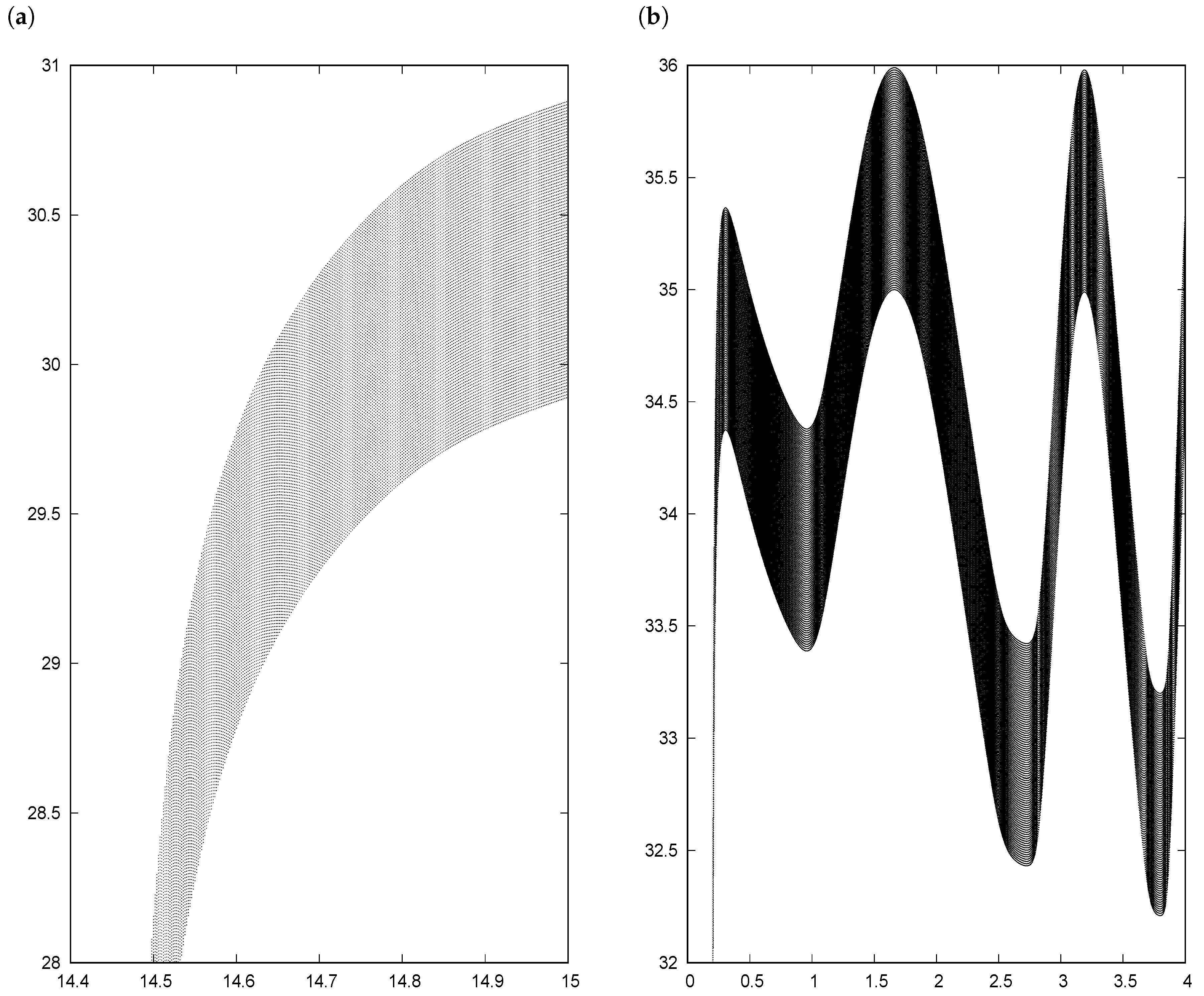
with different values of the initial condition and discarding the first 3000 iterations keeping the following one hundred iterations. When that finite number of iterations is displayed on the bifurcation diagram, oscillations appear. The resulting bifurcation diagrams show a behavior consisting in a wide collection of oscillatory functions for which the number of waves or bumps seems to depend on the initial condition. Such number of bumps and their amplitudes increases when the value of the initial condition decreases, see
Figure 2. It is important to remark that this behavior is not aperiodic or chaotic. What is most important, the system behaves as
for larger values of
Thus, the oscillatory behavior is preserved. This ghost bump phenomenon is analogous to the Gibbs phenomenon of a Fourier series [
17,
18]. Let us explain briefly this analogy. Gibbs phenomenon is an overshoot of an eigenfunction series approximation occurring at discontinuities of a piecewise continuously differentiable periodic function. Whereas the perturbed system approximates an unknown function with also unknown smoothness properties. Both, the Gibbs phenomenon and the ghost bump phenomenon, reflect the difficulty inherent in approximating numerically a function. The first by a truncated series of a combination of sine and cosine functions and the second by a truncated exponential polynomial which we will discuss next. It is important to remark that numerical simulation methods require stabilization methods when modeling oscillation phenomena. Since numerical overshoot is observed when the error tolerances are too loose and disappear for standard tolerances. Tighter tolerances lead to more accurate results, but increase the computational load. Gibbs phenomenon can can be reduced with a sigma approximation, see [
19]. For our case we still do not know if it is possible to stabilize our numerical procedure.
Let us show the reasons for the appearance of the oscillatory behavior. The perturbed system can be written as:
Each term in the sum contributes to generate a new bump in the graph of the function . Thus, For fixed n, the graph of the function will have bumps and then it will decay exponentially, with as rate of decay, to the value . Notice that the terms in the sum drop off quickly enough so the new iteration will inherit the previous bumps.
Regarding the variation of the initial condition, let us notice that the graph of
for fixed
n and fixed initial condition is compressed from the right, as compared with the graph for the same
n but with a smaller initial condition. Therefore, the initial condition indicates how frequently the function oscillates, playing a similar role as the angular frequency for harmonic oscillators [
20].
It is important to remark that the behavior shown for system (
1), is shared by many discrete exponential polynomial systems. Thus, an open question rises if such families act with accordance to a set of universal properties which are independent of the specific exponential polynomial considered. We should like briefly to illustrate this fact by way of the following example. Let us only modify the coefficients on the perturbed system in order to get a similar asymptotic behavior as system (
1). Let us replace the term
by the term
in the system (where
c is a constant). This modification makes the amplitude of the oscillations changed considerably. Moreover, the oscillation only appears when the constant
c is less than 2 and for larger values of the parameter, see
Figure 3a. Finally, if we replace now the term
by the term
in the perturbed system (where
d is a constant) the fixed point now becomes
, which is stable for
This new system also presents oscillations for most values of
d, see
Figure 3b. Therefore, we conclude that the exponential polynomial is the main cause of oscillations.
5. Conclusions
The study and analysis of exponential polynomial discrete dynamical systems is a new trend in Applied Computational Mathematics. One of the fundamental properties of a system is its structural stability, which means that the qualitative behavior of its trajectories is unaffected by small perturbations. In this work we have shown that a family of these system does not posses such a property even for constant perturbations. Our methodology used for this research was to show numerically and analytically the loss of stability of the unique fixed point for the perturbed system. We have discovered and established that polynomial discrete systems are complicated to analyze and most of the times even the equilibria are impossible to be provided with explicit closed-forms. This fact makes hard to implement standard analysis techniques. In essence we relied on computational methods to analyse the family of interest. We have shown that these systems exhibit transient behavior that remained for large number of iterations which does not correspond to their asymptotic behavior. A characteristic that may led to wrong results if one is using only numerical calculations due to the impossibility of carry out an analytical process. In the end, the determinative fact that the iteration function is a combination of products of exponential functions and polynomials no matter what the degree are on the given polynomials, a given exponential function will eventually decay faster than the polynomials.
One of the unpleasant features when considering only a finite number of iterations is the appearance of numerical oscillations. We showed the main reasons for the appearance of such oscillatory behavior. So far we are not able to verified if the computer numerical truncation is another factor.
In summary, our analysis of the perturbed exponential family is just a starting point to develop a more general theory for general polynomial discrete dynamical systems. We have discovered that are new open research venues such as potential stabilization methods which is a future research project.


