1. Introduction
Evolutionary Algorithms (EAs) are considered to be one of the core methods applied in the area of computational intelligence [
1]. Generally, EAs constitute a class of the main global search tools which can be adapted to deal with many forms of nonlinear and hard optimization problems. Developing applicable versions of EAs is hugely required to meet the fast-growing of optimization applications in all aspects of science [
2,
3]. Recently, there is an extreme interest in adapting EAs to be used with other computational intelligence techniques in different application areas. Although there are a vast number of attempts to modify the EAs to solve global optimization problems, most of them invoke only heuristic design elements, and they do not use mathematical mechanisms [
4,
5].
On the other hand, EAs have been applied in various optimization problems such as continuous, discrete, and combinatorial problems with and without constraints as well as mixed optimization problems [
6,
7]. Moreover, EAs are considered to be a milestone in the computational intelligence filed [
8]. Thus, developing practical schemes of EAs is remarkably required to meet the fast increasing of many applications in different real-life science [
2,
9]. However, EAs still have no automatic termination criteria. Thus, EAs algorithms cannot determine when or where they can terminate, and a user should pre-specify a criterion for that purpose. Typically, methods of termination criteria are such as when there has been no improvement in a pre-specified number of generations, when reaching a pre-specified number of generations, or when the objective function value has reached a pre-specified value. Another important designing issue is that controlling the randomness of some evolutionary operations should be considered in designing effective evolutionary-based search methods. This has motivated many researchers and was one of the main reasons for inventing the “memetic algorithms” [
10,
11]. Moreover, more deterministic operations have been highly recommended in developing the next generation genetic algorithms [
12].
The main goal of this research is to construct an effective and intelligent method that looks for optimal or near-optimal solutions to non-convex optimization problems. A global search method is to solve the general unconstrained global optimization problem:
In Equation (
1),
f is a real-value function that is defined in the search space
with variables
. Many methods of EAs have been suggested to deal with such problems [
13,
14]. This optimization problem has also been considered by different heuristic methods such as; tabu search [
15,
16,
17], simulated annealing [
18,
19,
20], memetic algorithms [
11], differential evolution [
21,
22], particle swarm optimization [
23,
24], ant colony optimization [
25], variable neighborhood search [
26], scatter search [
27,
28] and hybrid approaches [
29,
30,
31]. Multiple applications in various areas such as computer engineering, computer science, economic, engineering, computational science and medicine can be expressed or redefined as problem in Equation (
1), see [
2,
32] and references therein. The considered problem is an unconstrained one; however, there are several constraint-handling techniques that have been proposed to extend some of the previously mentioned research to deal with the constrained version of Problem (
1) [
33,
34,
35]. Some of the common techniques are to use penalty functions, fillers and dominance-based technique [
36,
37].
In this research, the proposed methods are expressed using quadratic models that partially approximate the objective function. Two design models have been invoked to construct these methods. In the first model called Quadratic Coding Genetic Algorithm (QAGA), trial solutions are encoded as coefficients of quadratic functions, and their fitness is evaluated by the objective values at quadratic optimizers of these models. Through generations, these quadratic forms are adapted by the genetic operators: selection, crossover, and mutation. In the second model, Evolution Strategies (ESs) are modified by exploiting search memory elements, automatic sensing conditions, and a quadratic search operator for global optimization. The second proposed method is called Sensing Evolution Strategies (SES). Specifically, the regression method and Artificial Neural Networks (ANN) are used as an approximation process. Explicitly, Radial Basis Functions (RBFs) are invoked as an efficient local ANN technique [
38].
The obtained results show that the quadratic approximation and coding models could improve the performance of EAs and could reach faster convergence. Moreover, the mutagenesis operator is much effective and cheaper than some local search techniques. Furthermore, the final intensification process can be started to refine the elite solutions obtained so far. In general, the numerical results indicate that the proposed methods are competitive with some other versions of EAs.
The rest of this paper is structured as follows. Related work is discussed in
Section 2. In
Section 3, the components of the proposed quadratic models are illustrated. The details of the proposed methods QCGA and SES are explained in
Section 4 and
Section 5, respectively. In
Section 6, numerical experiments aiming at analyzing and discussing the performance of the proposed methods and their novel operators are presented. Finally, the conclusion makes up
Section 7.
2. Related Work
The main contributions of this research are to use the wise guidance of mathematical techniques through quadratic models and to design smarter evolutionary-based methods that can sense the progress of the search to achieve finer intensification, wider exploration, and automatic termination.
In designing the proposed methods, EAs are customized with different guiding strategies. First, an exploration and exploitation strategy is proposed to provide the search process with accelerated automatic termination criteria. Specifically, matrices called Gene Matrix (GM) are constructed to sample the search space [
1,
39,
40]. The role of the
GM is to aid the exploration process. Typically,
GM can equip the search with novel diverse solutions by applying a unique type of mutation that is called “mutagenesis” [
39,
40]. Principally, mutagenesis may be defined as a nature mechanism by which the genes of an individual are changed, which lead to the mutation process. Thus, this mechanism is a driving force of evolution process [
40]. Thus, the mutagenesis operator alters some survival individuals to accelerate the exploration and exploitation processes [
40]. On the other hand,
GM is used to lead the search process to know how far the exploration process has gone to judge a termination point. Moreover, the mutagenesis operation lets the proposed method, the GA with Gene Matrix, perform like a so-called “Memetic Algorithm” [
41,
42] to accomplish a faster convergence [
40].
Practical termination criteria are one of the main designing issues in EAs. Typically, research is scant of termination criteria for EAs. However, in [
43], an empirical method is used to determine the maximum number of needed generations by using the problem characteristics to converge for a solution. Moreover, eight termination criteria have been discussed in [
44] that proposed a way of using clustering techniques to test the distribution of specific generation individuals in the search space. Different search memory mechanisms have been adapted as termination criteria to reflect the wideness of the exploration process [
39,
40,
45]. There are four classes of termination criteria of EAs [
39]. The first class is called
criterion, and it is based on calculating the best fitness function values over generations. This method keeps tracking the best fitness function values in each generation, and it terminates the algorithm if the values do not significantly change [
46,
47]. A
criterion is the second class measuring the population over generations. In each generation, the distances between chromosomes are measured and used to terminate the algorithm if these distances are very close. Work in [
48] uses
criterion for termination by adding distances among individuals and making sure it is smaller than a predefined threshold. The other two classes are
and
. The
criterion applies a computational budget such as the maximum number of generations or function evaluations for termination [
49,
50,
51]. In the
criterion, a search feedback measure evaluates the exploration and exploitation processes. Measures such as the distribution of the generated solutions or the frequencies of visiting regions inside the search space are invoked to test the search process. In [
45], the exploration process is examined by a diverse index set of points created at the beginning of the search process, which tries to guarantee a well-distribution of the generated points over the search space. The algorithm is terminated when most of the regions get visited.
These termination criteria may struggle from some difficulties [
45,
52]. Applying
only in EAs can easily make it trapped in local minima. Also, it is costly to have the entire population or a part of it convergent when using
, while it is sufficient to have one chromosome closely reach the global minima. Gaining prior information about the search problem is a big concern when invoking
criteria. Lastly, however using
looks effective; it may suffer the dimensionality problem, and it is complex to save and test huge historical search information. Therefore, implementing mixed termination criteria in EAs to overcome these problems is appreciated [
53,
54].
Evolutionary computing and artificial neural networks are main classes in computational intelligence [
55,
56]. Most of the research focus on how to use EAs to get more trained ANN [
57,
58]. There is relatively little research studying how to do the opposite by using ANN to design better EA-based methods or even to construct global optimization methods such in [
59,
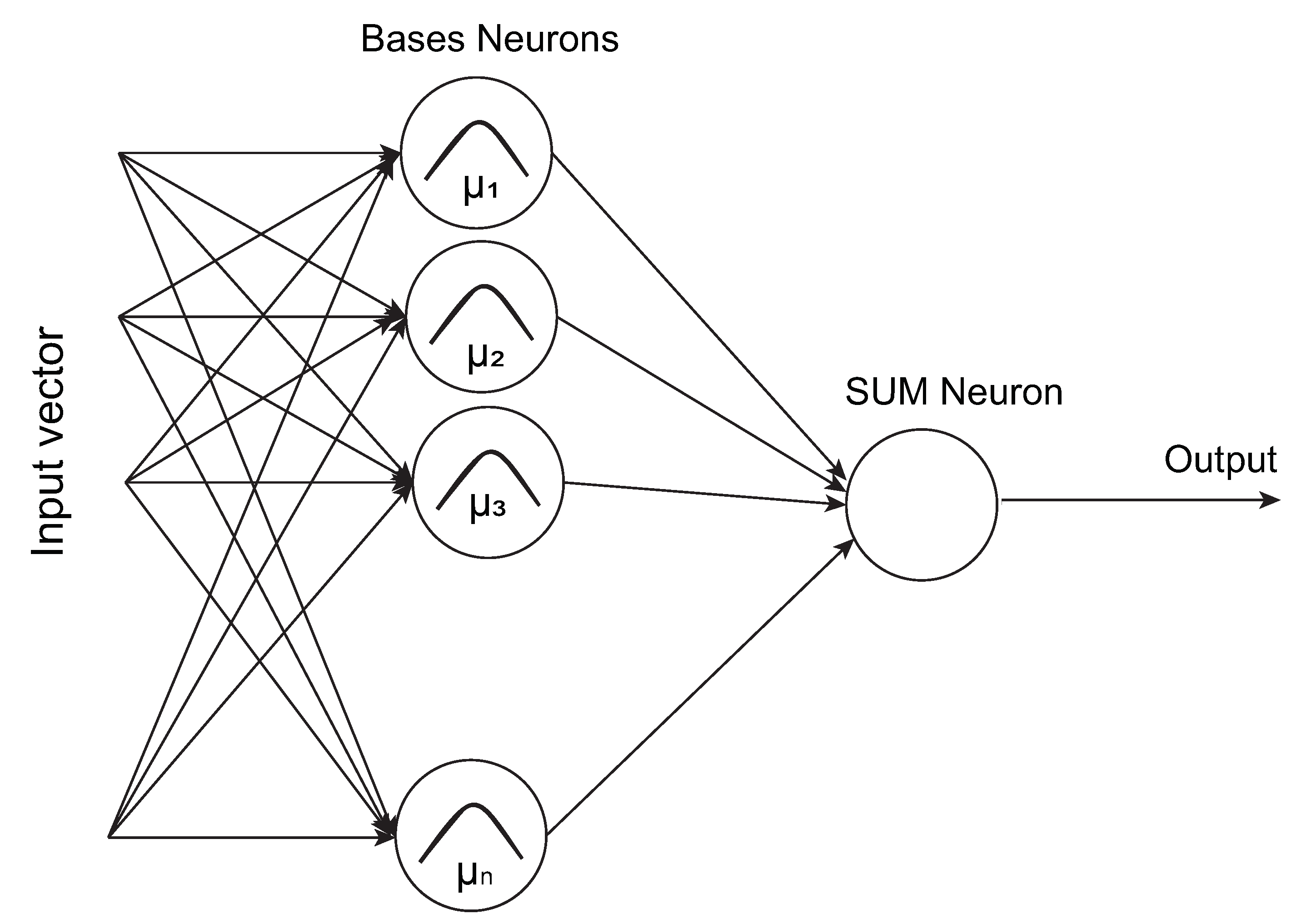
60]. In this research, the Radial Basis Functions (RBFs) are invoked as an efficient local ANN technique to help the EAs to reach promising regions and directions. Generally, other types of ANN could be used for the same task, such as the well-known multi-layer perceptron (MLB) with a training algorithm such as the back-propagation algorithm. However, RBFs is a local learning ANNs that could overcome the problem of long iterations learning process of other types of ANNs. In RBFs, the number of iterations is bounded maximum to the number of input samples. In other words, the middle layer adds one neuron per any new input sample, as shown in
Figure 1.
3. Quadratic Approximation Methods
One of the main steps in the proposed algorithms is to find out the best and fastest approximation for a high-dimensional function. Generally, two methods have been applied for this purpose; quadratic regression and radial basis function as a local supervised ANN. In both methods, the following Equation (
2) and its derivative are used for the fitting of the parameters:
where
A is an
matrix,
b is a vector with
n-dimension, and
c is a scalar. These individuals’ quadratic forms are adapted by the genetic operators through generations to fit the given objective function locally.
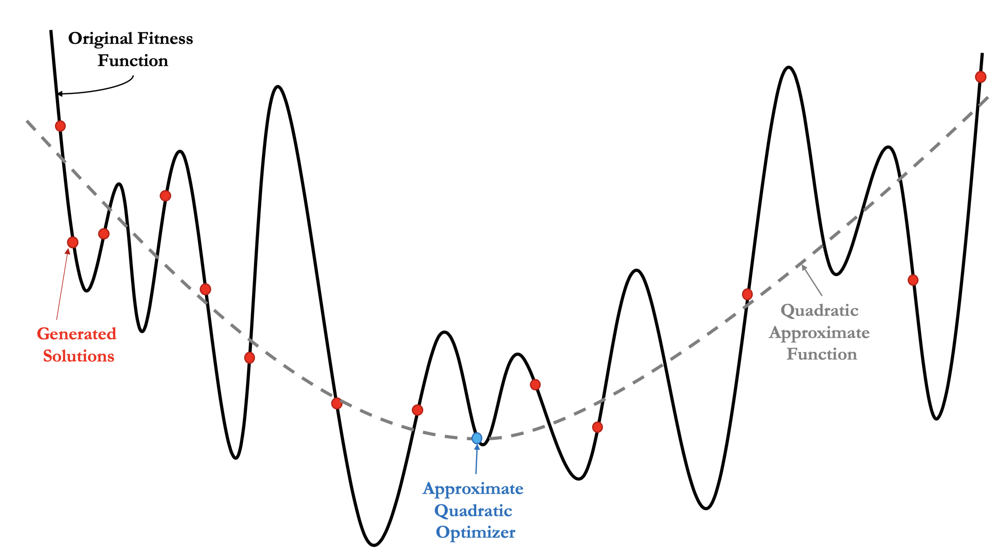
The least-square quadratic regression (also known as a nonlinear or second-order regression) is used because it is a fast and simple method for fitting. Moreover, it produces a good approximation and has very encouraging properties that can solve high-dimensional functions by finding
A,
b, and
c in Equation (
2). Thus, the idea is to choose a quadratic function that minimizes the sum of the squares of the vertical distances between the original fitness function values at generated solutions and an approximate quadratic function with finding coefficients
A,
b and
c, as shown in
Figure 2. Then, approximate quadratic optimizers of the quadratic models can be given by Equation (
3), which is represented by the derivative of Equation (
2).
It is computationally expensive to compute the inverse of a full matrix
A in Equation (
3), especially for high dimension problems. Hence, it is recommended to apply an efficient relaxation method to approximate
A to a diagonal matrix. Therefore, an approximate quadratic solution can be given as:
where
and
are the entities of
A and
b, respectively, with
,
and
.
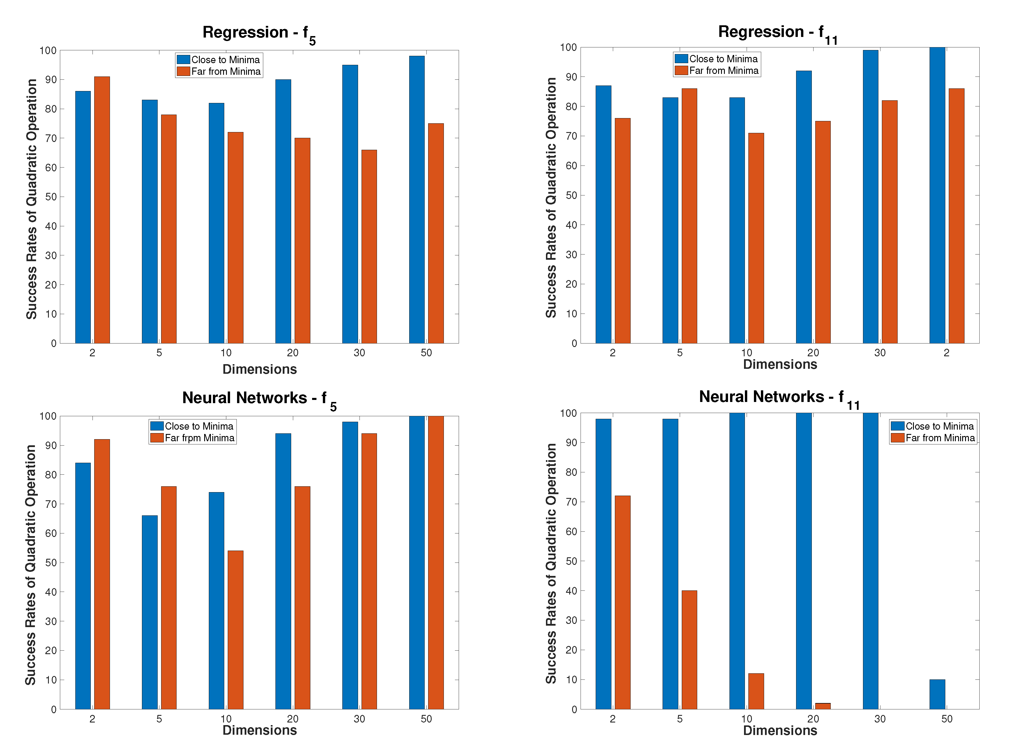
3.1. Regression
Quadratic regression models are usually generated using least-squares methods [
61]. Procedure 1 explains the steps of obtaining an approximate solution using the least-squares regression models. Starting with a set
S of previously generated solutions, the least-squares regression method is called to find an approximate quadratic function, as in Equation (
2), that fits those solutions. Then, an approximate optimizer can be calculated using Equation (
3).
Procedure 1. - 1.
Using least-squares regression, generate a quadratic model as in Equation (2) that fits the solutions in the sample set S. - 2.
Get the coefficients A, b, and c, of the generated approximate quadratic function.
- 3.
Return with the minimum point of the approximate quadratic function using Equations (3) and (4).
3.2. Artificial Neural Networks
Artificial Neural Networks (ANNs) are used in various optimization applications, such as in the areas of complex nonlinear system identification and global approximation. Many researchers have proved that multi-layer feed-forward ANNs, using different types of activation functions, works as a universal approximator [
38]. Moreover, continuous nonlinear functions can be approximated and/or interpolated with feed-forward ANNs and can be used to approximate the outputs of dynamical systems directly. Generally, ANNs are employed with EA in two main ways. Typically, most research focus on optimizing ANNs parameters, especially weights, using evolutionary techniques, especially GA [
62]. These results, in better classification of the ANNs, use of the power of both methods, the learning ability of the ANNs, and the best parameter values of EA. On the other hand, little research, such as this one, do the opposite thing by optimizing the evolutionary algorithms using ANNs for various purposes [
63,
64,
65].
In this research, the speedup of the optimization process has been done using an RBF neural network. The RBF has been used for searching for the approximated quadratic function for a continuous function of variables such as shown in
Appendix A and
Appendix B. Therefore, The RBF builds local representations of the functions and so their parameters. However, RBFs are simpler to be initialized and trained than feed-forward multi-layer perceptrons (MLPs) neural networks. Thus, RBFs overcome the problem of the training iteration process as it is a local learning type of neural network. Therefore, the iterations are bounded as a maximum of the number of input samples. However, RBFs approximation may be very attractive for approximating complex functions in numerical simulations. Moreover, RBFs would allow randomly scattered data to generalize easily to several space dimensions, and it can be accurate in the interpolation process. With all those motivations, this study used the properties of RBFs approximations to develop a new global optimization tool.
As shown in
Figure 1, the RBF neural network is a two-layer ANN, where each hidden unit exploits a radial (Gaussian) activation function for the hidden layer processing elements. The output unit applies a weighted sum of all hidden unit outputs. Although the inputs into the RBF network are nonlinear, the output is linear due to the structure of the RBF neural network. By adjusting the parameters of the Gaussian functions in the hidden layer neurons, each one reacts only to a small region of the input space. However, for successful performance and implementation of RBFs is to find reasonable centers and widths of the Gaussian functions. In this research, during simulation, a MATLAB function is used to determine the Gaussian centers and widths using the input data of the desired function from
Appendix A and
Appendix B. Once the hidden layer has completed its local training and all parameters adjustment, the output layer then adds the outputs of the hidden layer based on its weights. The steps of obtaining an approximate solution using the ANN models are shown in Procedure 2.
Procedure 2. - 1.
A set S of generated samples of solutions is used for training the RBF to obtain an approximate quadratic function as in Equation (2). - 2.
Get the coefficients A, b and c of the approximate quadratic function obtained by the RBF network.
- 3.
Return with the minimum point of the approximate quadratic function using Equations (3) and (4).
4. Quadratic Coding Genetic Algorithm
One of the proposed methods in this research is called the Quadratic Coding Genetic Algorithm (QCGA). In the following, the main structure and design of the proposed QCGA method are described. Generally, the QCGA method uses a population of
individuals or solutions. Each individual represents a quadratic form model as in Equation (
2). These quadratic form individuals are adapted by the genetic operators through generations to fit the given objective function locally. Therefore, optimizing these quadratic models can provide approximated solutions for the local minima of a given objective function. The optimizers of the quadratic models can be given by Equation (
3), as explained before.
Practically, it is very costly to compute the inverse of a full matrix
A in Equation (
3), especially for high dimension problems. Hence, using a reasonable relaxation form of this coefficient matrix is crucial. Thus, as a main step in the proposed method,
A is approximated as a diagonal matrix. Therefore, the QCGA individuals are coded in the quadratic models as:
where
are equal to the diagonal entities of
A,
are equal to the entities of
b, and
. To avoid the non-singularity of
A, the entities
are initialized and updated to satisfy the conditions
, for some predefined small real number
. The individuals fitness values are computed as
, where
is the given objective function and
is calculated as:
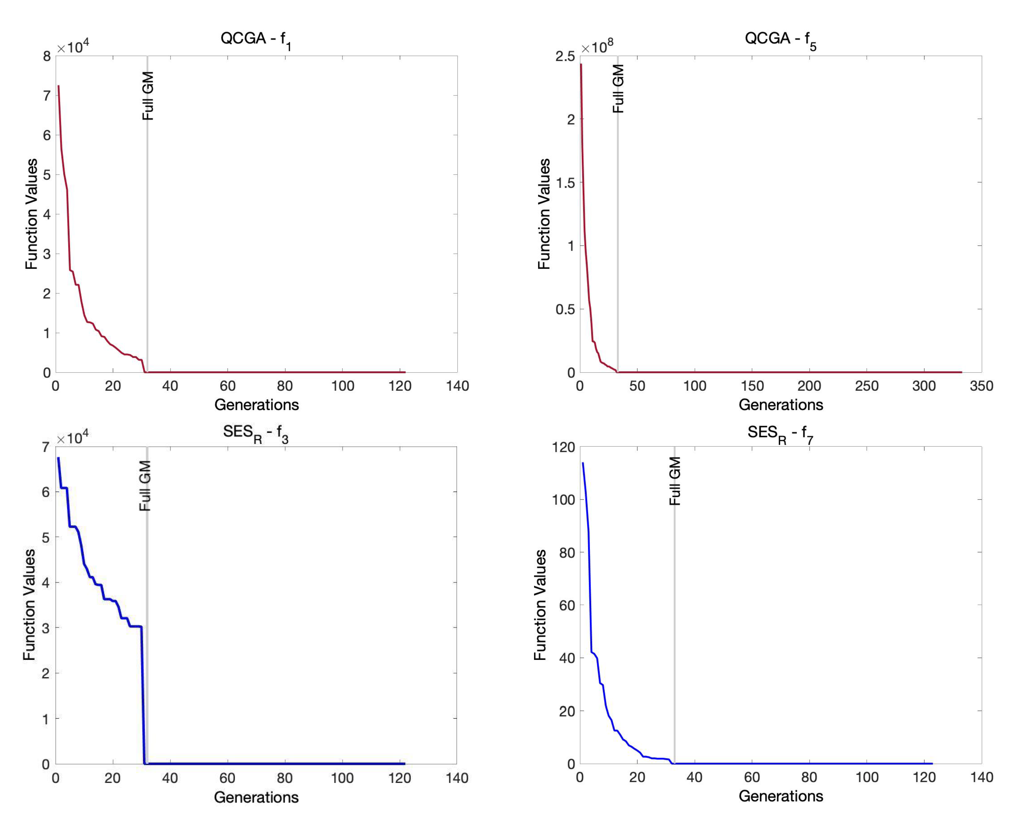
The algorithmic scenario of QCGA is shown in
Figure 3. In each iteration of the QCGA algorithm, an intermediate parent population is generated using the linear ranking selection mechanism [
66]. Then, the arithmetical crossover and uniform mutation operators [
67] are applied to reproduce the offspring. After getting the children, the survival selection is applied to select the survival members based on the members’ elitism. Finally, the QCGA uses local search methods of Nelder–Mead [
68] and the heuristic descent method [
18] as a final intensification step to refine the best solutions found so far.
5. Sensing Evolution Strategies
The difficulty in solving global optimization problems arises from the challenge of searching a vast variable space to locate an optimal point, or at least space of points, with appropriate solution quality. It becomes even more challenging when the appropriate space is minimal compared to the complex search space. However, the quality of the initial solutions may impact the performance of the algorithm. Thus, various global optimization techniques which exploit memory concept in different ways to help in both finding the optimal solution in minimum time and reduce the problem complexity are proposed. Generally, memory concept is used in various research for the sake of assisting exploration and exploitation processes. In [
40], a directing strategy based on new search memories; the Gene Matrix (
GM) and Landscape Matrix (
LM) is proposed. That strategy can provide the search with new diverse solutions by applying a new type of mutation called “mutagenesis” [
39]. The mutagenesis operator is used to change selected survival individuals to accelerate the exploration and exploitation processes. However, the
GM and
LM are also used to help the search process to remember how far the exploration process has gone to judge a termination point. In [
15,
16], tabu search algorithms are used with memory concept in high-dimensional problems to explore the region around an iterate solution more precisely.
The main structure of the proposed Sensing Evolution Strategies (SES) is shown in
Figure 4. In the following, full details of the SES method and its algorithm steps are described. The SES method starts with a population of
real-coded chromosomes. The mutated offspring is generated as in the typical ESs [
69,
70]. Therefore, a mutated offspring
is obtained from a parent
, where the
i-th component of the mutated offspring
is given as:
where
and
, and the proportional coefficients are usually set to one. The mutated offspring can be also computed from recombined parent as given in Procedure 3.
Procedure 3. - 1.
If then return.
- 2.
Partition each parent into ρ partitions at the same positions, i.e., , .
- 3.
Order the set randomly to be .
- 4.
Calculate the recombined child , and return.
Adding sensing features to the proposed SES method makes it behave smarter. This can be achieved by generating and analyze search data and memory elements. As a main search memory for the SES, the
GM is invoked as it has shown promising performance in global optimization [
1,
39,
40]. In
GM, each
x in the search space consists of
n genes or variables to get a real-coding representation of each individual in
x. First, the range value of each gene is divided into
m sub-range to check the diversity of the gene values. Thus, the
GM is initialized to be a
zero matrix in which each entry of the
i-th row refers to a sub-space of the
i-th gene, from which
GM is zeros, and ones matrix and its entries are changed from zeros to ones if new genes are generated within the corresponding sub-spaces during the searching process, as shown in
Figure 5. This process can be continued until all entries become ones, i.e., with no zero entry in the
GM. At that point, when the
GM is considered full of ones, the search process achieves an advanced exploration process and can be stopped. Therefore, the
GM is used to provide the search process with efficient termination criteria, and it can help by providing the search process with various diverse solutions.
Three sensing features have been invoked in the SES method as explained in the following:
Intensification Sensing. This feature seeks to detect promising search regions that have been recently visited. Then, a local fast search can be applied to explore such promising regions deeply. The SES method uses quadratic search models as stated in Procedures 1 and 2 to obtain approximate premising solutions using Equation (
4). Moreover, a promising region can be detected when the generated mutated children are adapted to be close. Then, a quadratic model can be generated to approximate the fitness function in that close region surrounding those mutated children.
Diversification Sensing. This feature aims to avoid entrapment in local solutions and recognize the need for generating new diverse solutions. The SES method checks the improvement rates while the search is going on. Whenever significant non-improvement has been faced, then the mutagenesis operation (Procedure 4) is called to generate new diverse solutions. In that procedure, new solutions are created by generating their gene values within sub-ranges whose corresponding indicators are zeros in the
GM as shown in
Figure 6. Those diverse solutions replace some worst solutions in the current population.
Exploration Sensing. This feature tries to recognize the progress of the search exploration process and to detect an appropriate time for termination whenever a wide exploration process is achieved. When a full GM is reached, then the SES method has learned that the exploration method is almost over.
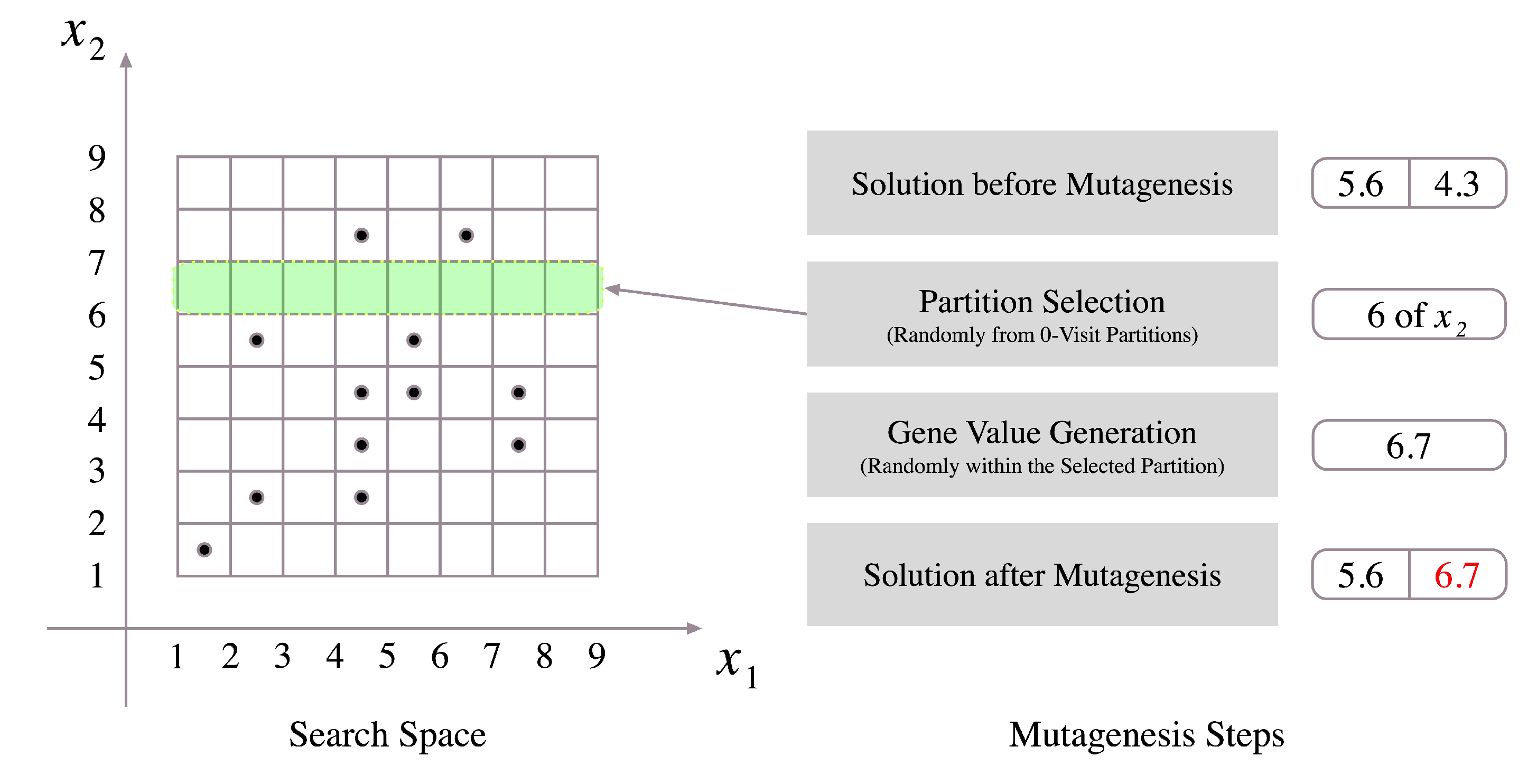
The mutagenesis operation starts with selecting a zero-position in the
GM, which is corresponding to a zero-visit partition. Selecting such
GM-entry is done randomly. Then, a new value of the gene related to the selected
GM-entry is generated within the corresponding partition of the selection, as illustrated in
Figure 6. The formal description of this mechanism is stated in Procedure 4.
Procedure 4. - 1.
If GM is full then return.
- 2.
Choose a zero-position in GM randomly.
- 3.
Update x by setting , where r is a random number from , and are the lower and upper bound of the variable , respectively.
- 4.
Update GM by setting , and return.
The formal description of the proposed SES method is given in the following Algorithm 1.
Algorithm 1. SES Algorithm - 1.
Initialization.Create an initial population and initialize the GM. Choose the recombination probability , set values of; ρ, and , set , and set the generation counter .
- 2.
Main Loop.Repeat the following steps (2.1)–(2.4) from
- 2.1
Recombination.Generate a random number If , choose a parent from and go to Step 2.2. Otherwise, choose ρ parents from , and calculate the recombined child using Procedure 3.
- 2.2
Mutation.Use the individual to calculate the mutated children as in Equations (7) and (8). - 2.3
Fitness.Evaluate the fitness function
- 2.4
Intensification Sensing.If the individual and his mutated children are close enough to be approximated by a quadratic model, the apply Procedure 1 or 2 to get an improved point. Replace the worst mutated child with the generated point by the quadratic model if the latter is better.
- 3.
Children Gathering.Collect all generated children in containing all
- 4.
Update Search Parameters. Update the GM.
- 5.
Exploration Sensing. If the GM is full, then go to Step 8.
- 6.
Selection.Choose the best μ individuals from to compose the next generation . Update the gene matrix GM.
- 7.
Diversification Sensing. If the new population needs new diverse solutions, then apply Procedure 4 to alter the worst individuals in . Set , and go to Step 2.
- 8.
Intensification.Apply a local search method starting from each solution from the best ones obtained in the previous search stage.
The non-convex global optimization problem, defined in Equation (
1), is an
-complete problem [
71]. Therefore, there is no efficient algorithm to solve such problem in its general form. Metaheuristics are practical solvers for this problem which are generally polynomial algorithms [
72,
73]. The proposed methods; QCGA and SES, follow the main structures of standard EAs with additive procedures which are at most of order
.
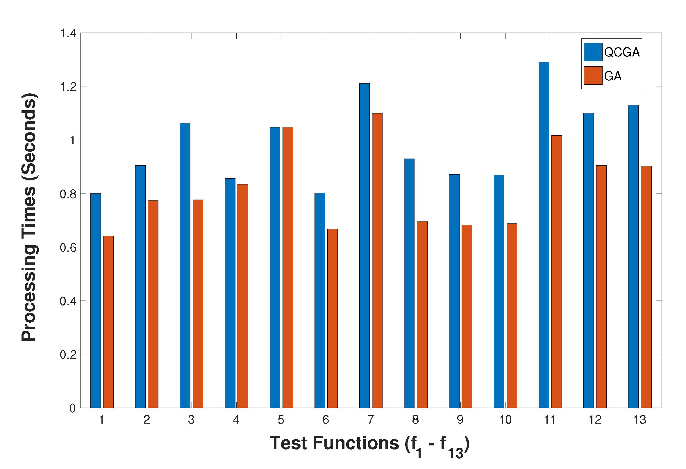
7. Conclusions
In this work, we propose a modified GA version called QCGA, which is based on applying a quadratic search operator to solve the global optimization problem. The use of quadratic coding of solutions efficiently assists the algorithm in achieving promising performance. Furthermore, other quadratic-based techniques are presented as search operators to help the ESs in finding a global solution quickly. Moreover, the gene matrix memory element is invoked, which could guide the search process to new diverse solutions and help in terminating the algorithms. The efficiency of these methods is tested using several sets of benchmark test functions. The comparisons with some standard techniques in the literature indicate that the proposed methods are promising and show the efficiency of them shortening the computational costs. We may conclude that applying quadratic search operators can give them better performance and quick solutions. Therefore, we suggest the extension of the proposed ideas to modify the other metaheuristics. The quadratic search models can be invoked as local search procedures in many methods such as particle swarm optimization, ant colony optimization, and artificial immune systems. Moreover, the quadratic models and coding can also be used in response surface and surrogate optimization techniques. Finally, the proposed methods can also be extended to deal with constrained global optimization problems using suitable constraint-handling techniques.


