Article

Investigation of Volumic Permanent-Magnet Eddy-Current Losses in Multi-Phase Synchronous Machines from Hybrid Multi-Layer Model

Département ENERGIE, FEMTO-ST, CNRS, Univ. Bourgogne Franche-Comté, F90000 Belfort, France
*
Authors to whom correspondence should be addressed.
Math. Comput. Appl. 2020, 25(1), 14; https://doi.org/10.3390/mca25010014
Submission received: 5 October 2019 / Revised: 29 February 2020 / Accepted: 4 March 2020 / Published: 4 March 2020
(This article belongs to the Special Issue Mathematical Models for the Design of Electrical Machines)

Abstract

:
This paper investigates the permanent-magnet (PM) eddy-current losses in multi-phase PM synchronous machines (PMSM) with concentric winding and surface-mounted PMs. A hybrid multi-layer model, combining a two-dimensional (2-D) generic magnetic equivalent circuit (MEC) with a 2-D analytical model based on the Maxwell–Fourier method (i.e., the formal resolution of Maxwell’s equations by using the separation of variables method and the Fourier’s series), performs the eddy-current loss calculations. First, the magnetic flux density was obtained from the 2-D generic MEC and then subjected to the Fast Fourier Transform (FFT). The semi-analytical model includes the automatic mesh of static/moving zones, the saturation effect and zones connection in accordance with rotor motion based on a new approach called “Air-gap sliding line technic”. The results of the hybrid multi-layer model were compared with those obtained by three-dimensional (3-D) nonlinear finite-element analysis (FEA). The PM eddy-current losses were estimated on different paths for different segmentations as follow: (i) one segment (no segmentation), (ii) five axial segments, and (iii) two circumferential segments, where the non-uniformity loss distribution is shown. The top of PMs presents a higher quantity of losses compared to the bottom.

1. Introduction

Currently, there is trend of the electrification of transport applications, where PMSM are increasingly being used. The reason is their good torque density, lower losses and higher power-to-mass ratio [1]. In addition to advantages associated to this topology, a multi-phase system allows continuous operation in degraded mode, which is a powerful asset in traction application [2,3].
One of the major concerns in PMSM is the PM demagnetization risk. This occur by temperature rise caused by the eddy-currents [4]. The high-order magnetic flux density harmonics, which are not synchronous with the rotor, cause those parasitic eddy-current losses in the PMs [5]. Eddy-current losses may be separated into two cases according to the operating point:
  • No-load (without stator current): the reluctance variation due to the stator slot-opening [5,6];
  • Load (with stator current): the spatio-temporal magnetomotive force (MMF) harmonics [7,8].
In design process, the PM eddy-current losses must be calculated. Several methods have been developed and categorized into three families viz.: (i) (Semi-)analytical methods based the formal resolution of Maxwell’s equations [9,10], (ii) numerical methods [11,12], and (iii) hybrid methods [13,14]. An overview on the eddy-current loss calculation has been realized in [15], where several investigations have been chronologically listed. In [16], sources, calculation methods, reduction techniques, and thermal analysis of PM eddy-current losses were revised. A review of (semi-)analytical models based on the subdomain technique for PM eddy-current calculation was made by [17].
The fact that the eddy-currents flow is along the loops inside the PM volume leads to the classification of their calculation as a 3-D problem [18]. The 2-D calculation ignores end-effects which cause a large error in the PM eddy-current computation. To consider end-effects and obtain a more accurate calculation, a 3-D model must be used [19].
This paper investigates the PM eddy-current losses in massive conducting parts of a multi-phase PMSM from hybrid multi-layer model. The latter consists of combining two models, viz.: (i) a 2-D generic MEC, and (ii) a 2-D analytical model based on the Maxwell–Fourier method (i.e., the formal resolution of Maxwell’s equations by using the separation of variables method and the Fourier’s series). The 2-D generic MEC determines the magnetic flux density distribution in the massive conductive parts (e.g., the PMs,...) without the skin effect (i.e., without the eddy-current reaction field). Moreover, this model can give the distribution of other local/integral physical quantities in the electrical machine with the nonlinear of B ( H ) curve. The 2-D analytical model based on the Maxwell–Fourier method calculates the magnetic field distribution in massive conductive parts considering the skin effect as well as the resultant eddy-current density. The boundary conditions (BCs) imposed on the 2-D analytical model are equivalent to the magnetic field obtained from the MEC. These BCs are considered homogeneous on the edges and are only equal to normal magnetic field in the top or middle of massive conductive parts. This is a strong hypothesis, because the magnetic field is naturally non-uniform. In our case, the model gives the ability to use both conditions (i.e., in the top or middle of massive conductive parts), allowing to see the impact on the eddy-current loss calculation.
Eddy-current losses are investigated on a multi-phase PMSM with a non-overlapping (i.e., concentrated) all-teeth wound winding (double-layer winding with left and right layer) having 5-phases/20-slots/16-poles [20].
The proposed approach is introduced in Section 2 with a short focus of the 2-D generic MEC and its validation. Section 3 shows the obtained PM eddy-current losses on different paths for different segmentations. In the last section, the results of the hybrid multi-layer model are compared with those obtained by 3-D nonlinear FEA [21].

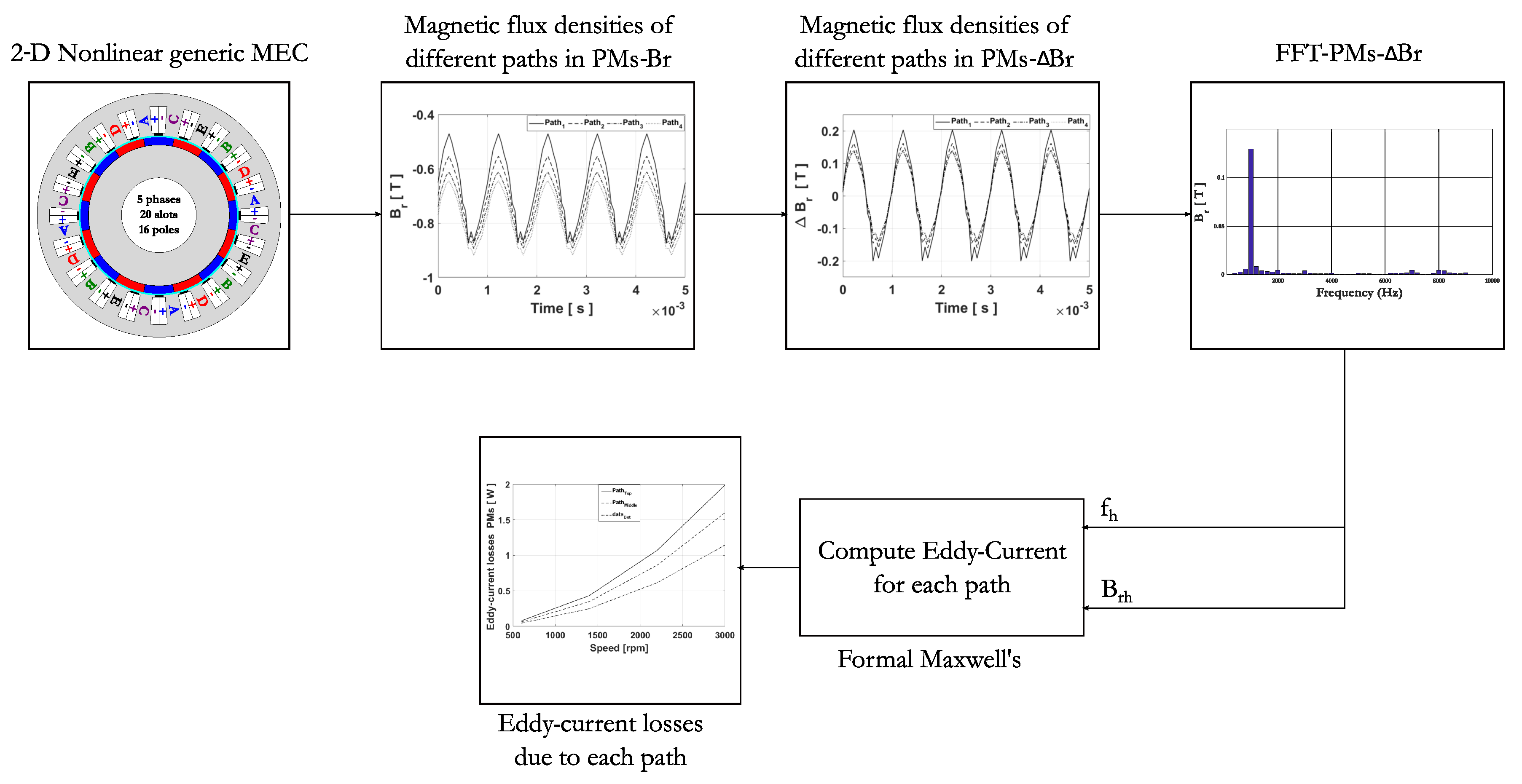
2. Hybrid Multi-Layer Model Description

The performed approach is composed of two main modules, viz.: (i) a 2-D generic MEC, and (ii) a 2-D analytical model based on the Maxwell–Fourier method. The first one allows the calculation of magnetic flux density B without the skin effect over all the PMSM. In the PM zones, the magnetic flux density is levied on different paths parallel in the tangential direction. Indeed, the magnetic flux density varies depending on the PM depth direction. These magnetic flux densities will be subjected to the FFT giving the amplitude as well as the frequency of different harmonic numbers. Furthermore, these outputs constitute the main input parameters to estimate the PM eddy-current losses by using the developed formal Maxwell model. Note that only the harmonics are going to be taken into account when calculating the eddy-current losses. The eddy-current losses due to the average value are null because the resultant eddy-current density in the PMs does not exist. The developed approach for the eddy-current loss calculation is explained in the flowchart shown in Figure 1.

2.1. Geometrical and Physical Parameters of PMSM

The performed model was applied to a five-phase surface-mounted PMSM, where the geometrical and physical parameters are given, respectively, in Table 1 and Table 2. Figure 2 gives the topology of the machine and the spatial distribution of various phases. The stator has a double-layer concentrated winding distribution (viz., the non-overlapping winding with all teeth wound), supplied by sinusoidal current waveform. The five-phases windings are star-connected. The PMs, radially magnetized, and the sheet metal are, respectively, NdFeB and M270-35A. The dashed lines represent the different paths used to proof this approach. Based on this path, the local quantities will be levied and furthermore compared to those of FEA [21].
Attention should be paid to Figure 3 which presents the different tangential paths located in both South and North PM. This path will be used to get the different values of the magnetic field along the symmetric axis of the PM.

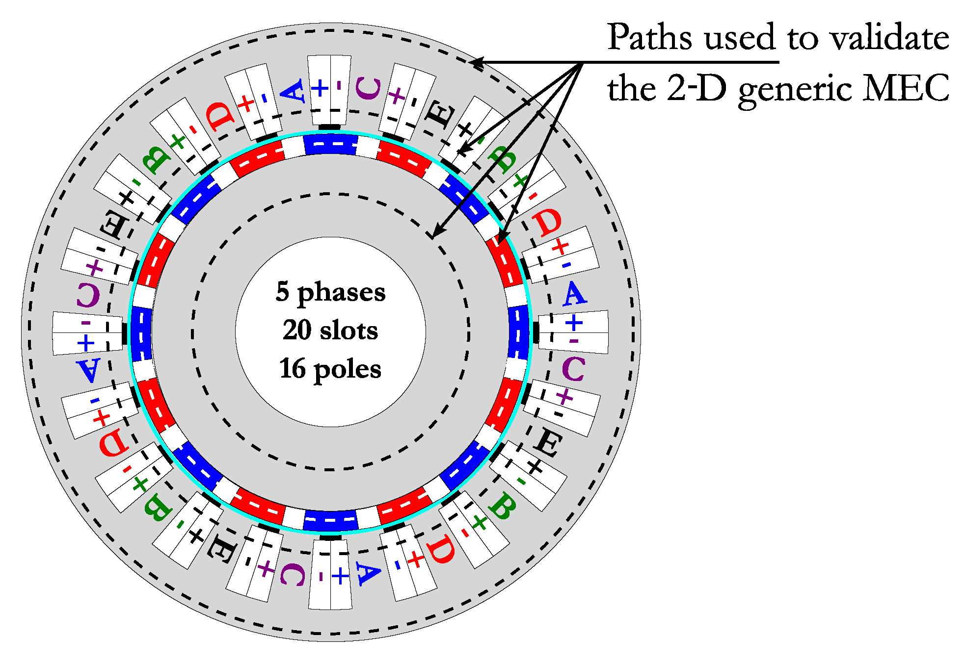
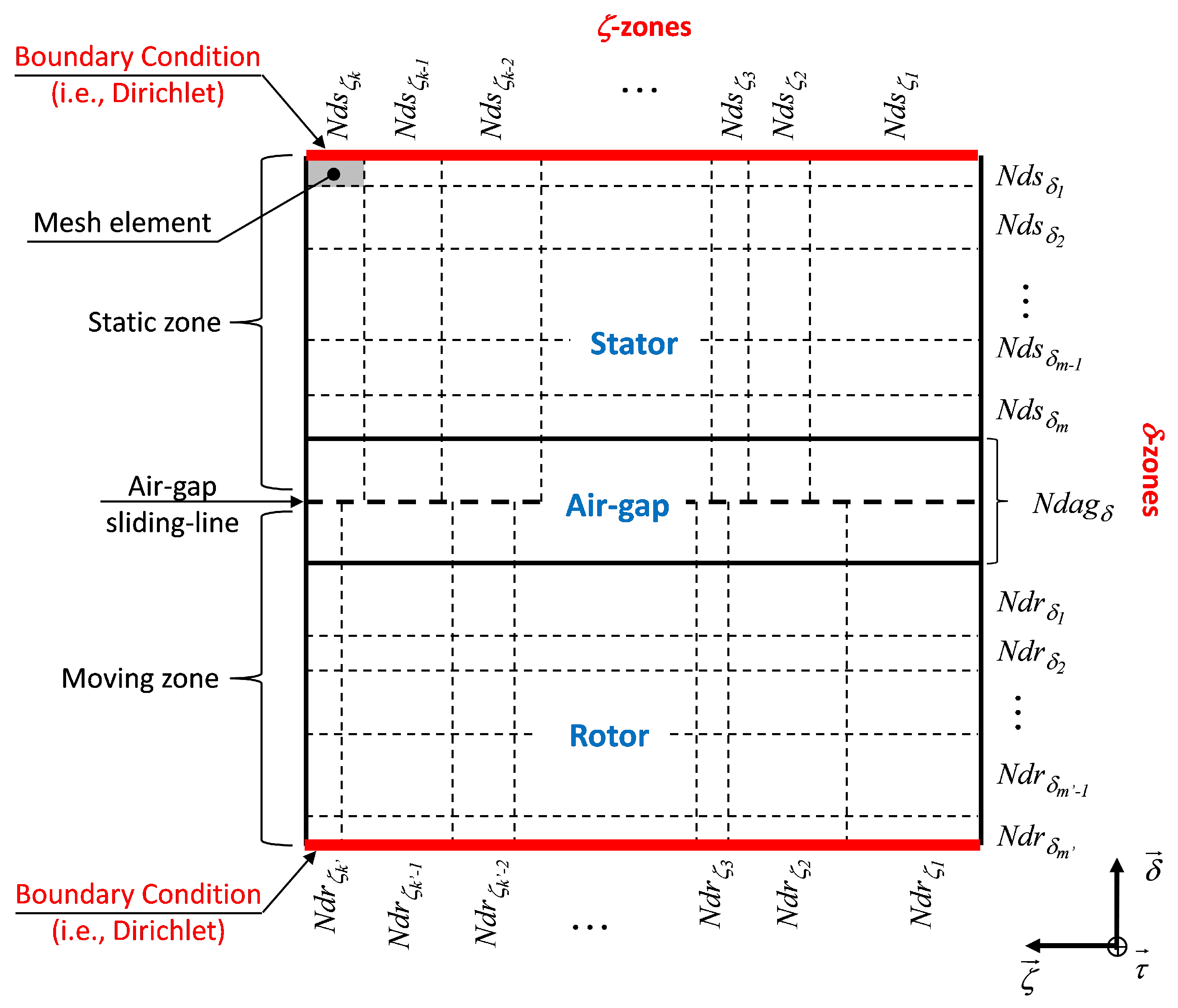
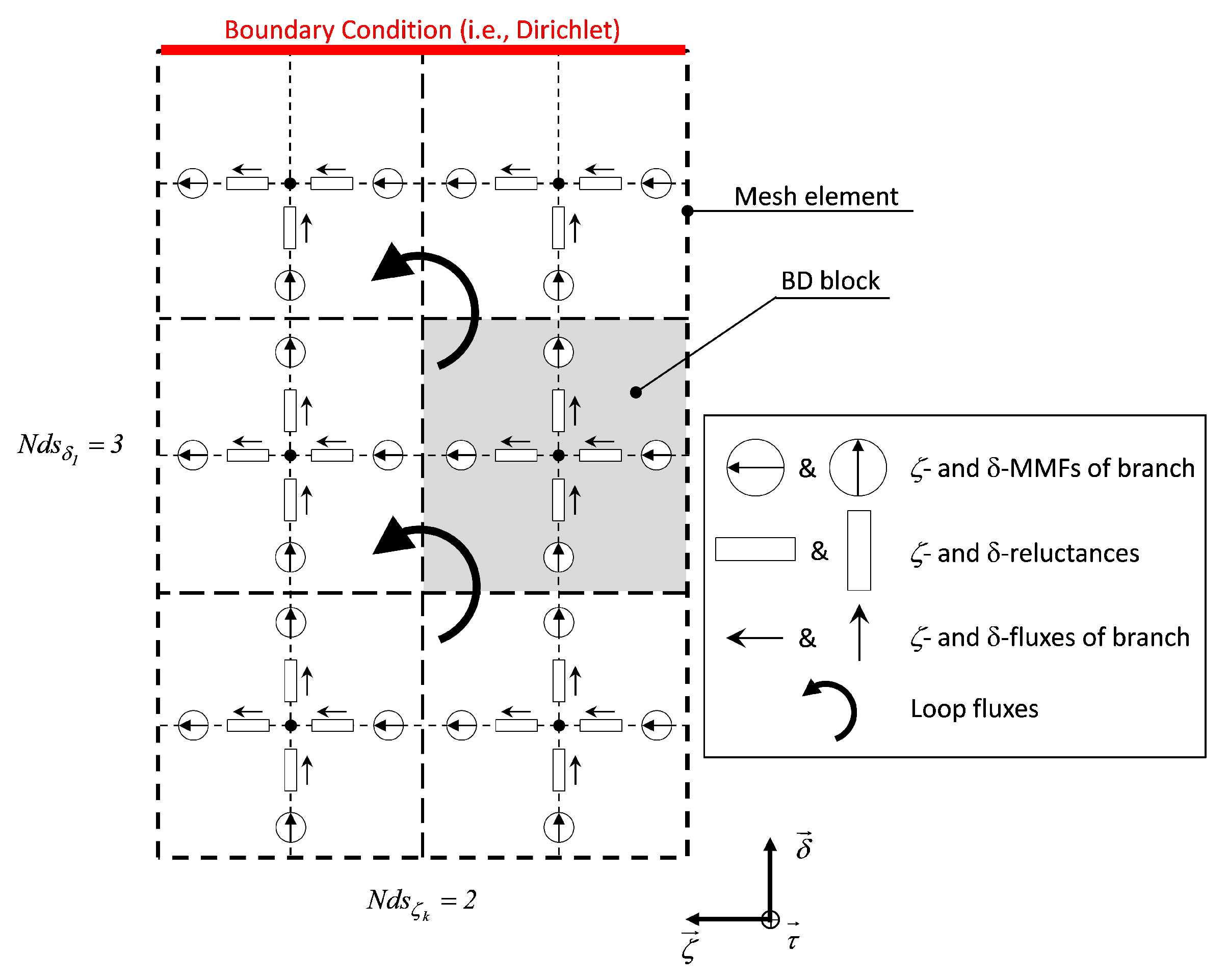
2.2. 2-D Generic MEC

In this work, the approach proposed in [22] (viz., the generalized nonlinear adaptive MEC) was applied onto the 5-phases PMSM. Indeed, the 2-D MEC is based on the discretization principle, which allows bidirectional (BD) automatic mesh reluctance generation. In a general manner, the electrical machine can be discretized in a set of mesh elements that can be, in turn, discretized in a high number of BD blocks. As an example, the mesh element spotted by the grey color in Figure 4 can be discretized in a set of BD blocks, as shown in Figure 5.
The main advantages of such a model include of the flexibility, generic, compromise between computation time and precision. The semi-analytical model includes the automatic mesh of static/moving zones, the saturation effect and zones connection in accordance with rotor motion based on a new approach called “Air-gap sliding line technic”. This technique was applied in [23,24,25,26] on different electrical machine configurations, viz., axial-flux interior PM machine [23,24], coaxial magnetic gear equipped with surface-mounted PMs [25], wound-rotor synchronous machine [27], and radial-flux interior PM machine [26]. This novel technique of connection between static/moving zones as well as the approach proposed in [22] is applied for the first time on a radial-flux surface-mounted PMSM having multi-phases for automotive application. Nevertheless, it should be noted that there are other techniques permitting to connect static/moving zones in electrical machines which have been overviewed in [22].
Comparing to [26], in our case, the stator tooth-pitch will be constituted by five radial zones, and four radial zones for the rotor pole pitch. For the tangential zones, the rotor pole pitch is consists of three zones, while the stator pitch consists of five zones. The discretization number in each zones is given by Table 3.
The developed model respects the flowchart given in Figure 6, where the different steps of the nonlinear system solving are presented. To account for the saturation effect, an iterative process is considered by using the fixed point iteration method. The nonlinear B(H) curve of the iron is then introduced by using the Marrocco’s interpolation function. In Figure 6, μ r i represents the initial relative permeability in the magnetic circuit and N s a t is the total iterations number for taking into account the saturation effect. The 2-D nonlinear adaptive MEC (where the loop fluxes ψ are the unknowns) can be expressed by
χ · · χ T · ψ F = 0 with F = χ · M M F
ϕ = χ T · ψ
where is the diagonal matrix of reluctances, ψ is the loop fluxes vector, χ is the topological (or incidence) matrix, F is the loop MMFs vector, and M M F is the branch MMFs vector. These matrixes and vectors are dependent upon the discretization of the various zones. Their dimensions are invariable with the time (or the mechanical angular position between the rotor and the stator) [22]. Finally, dividing this later by the corresponding reluctance surfaces leads to the magnetic flux density in each magnetic branch.

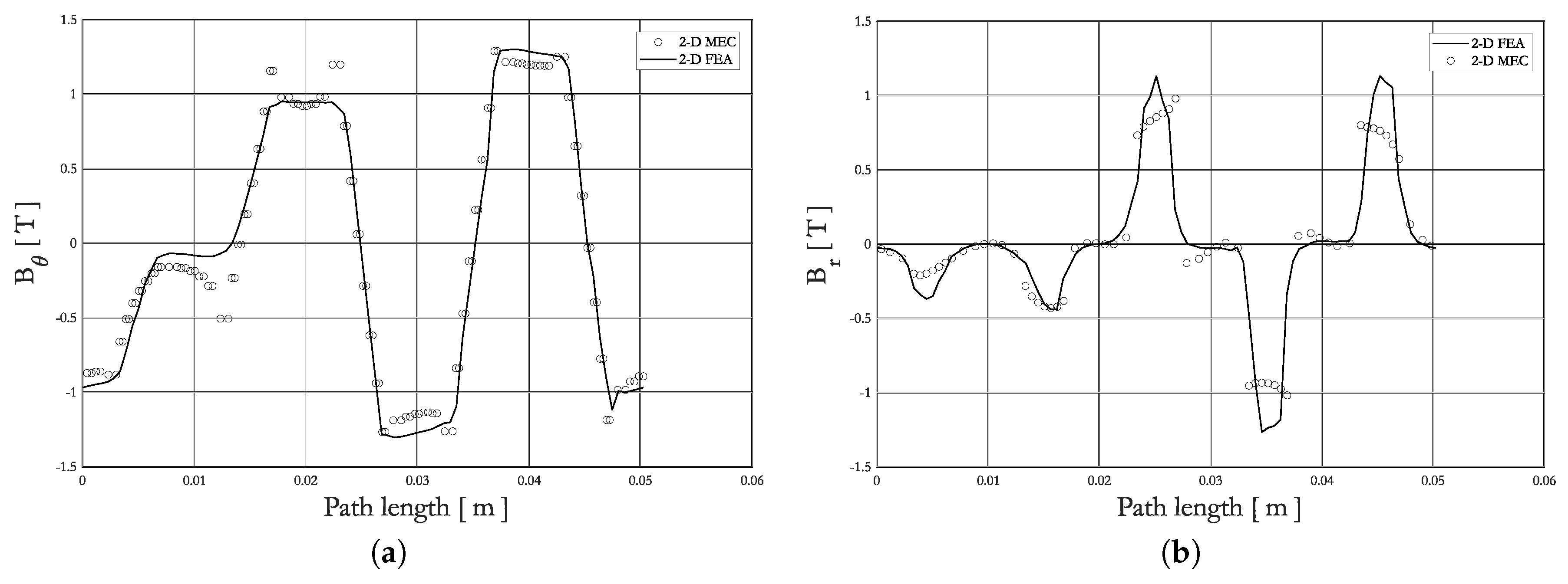
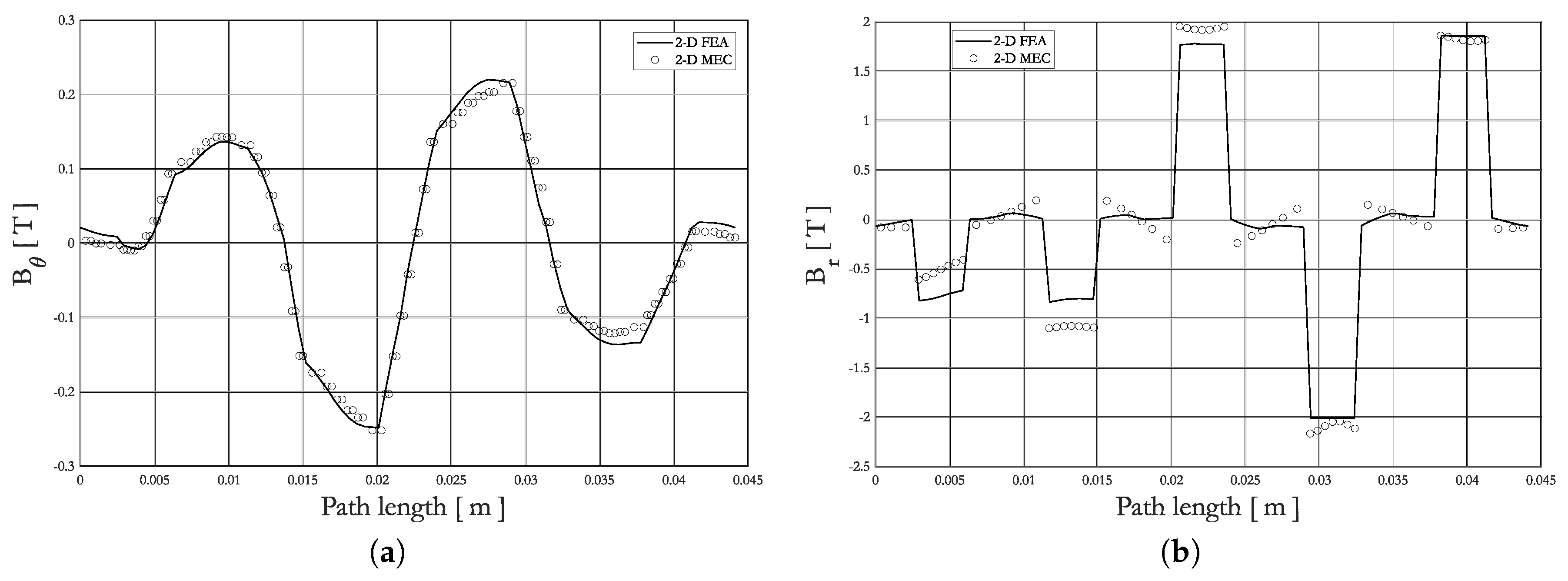
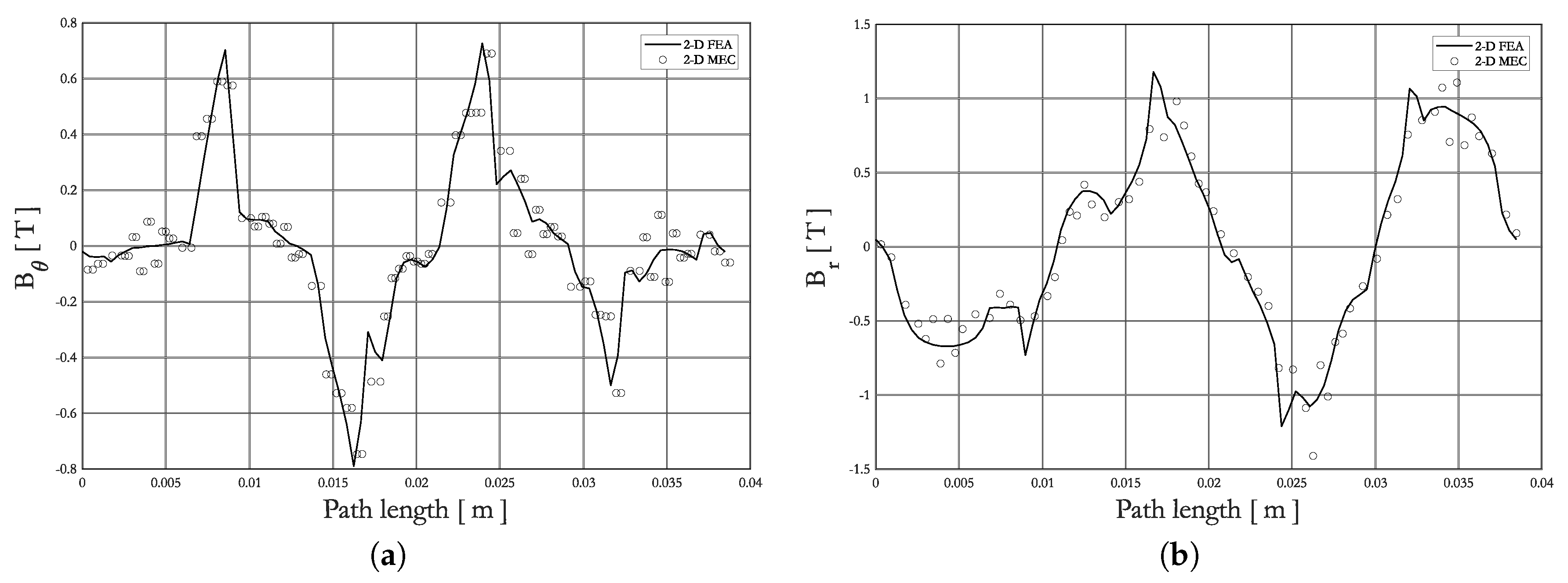
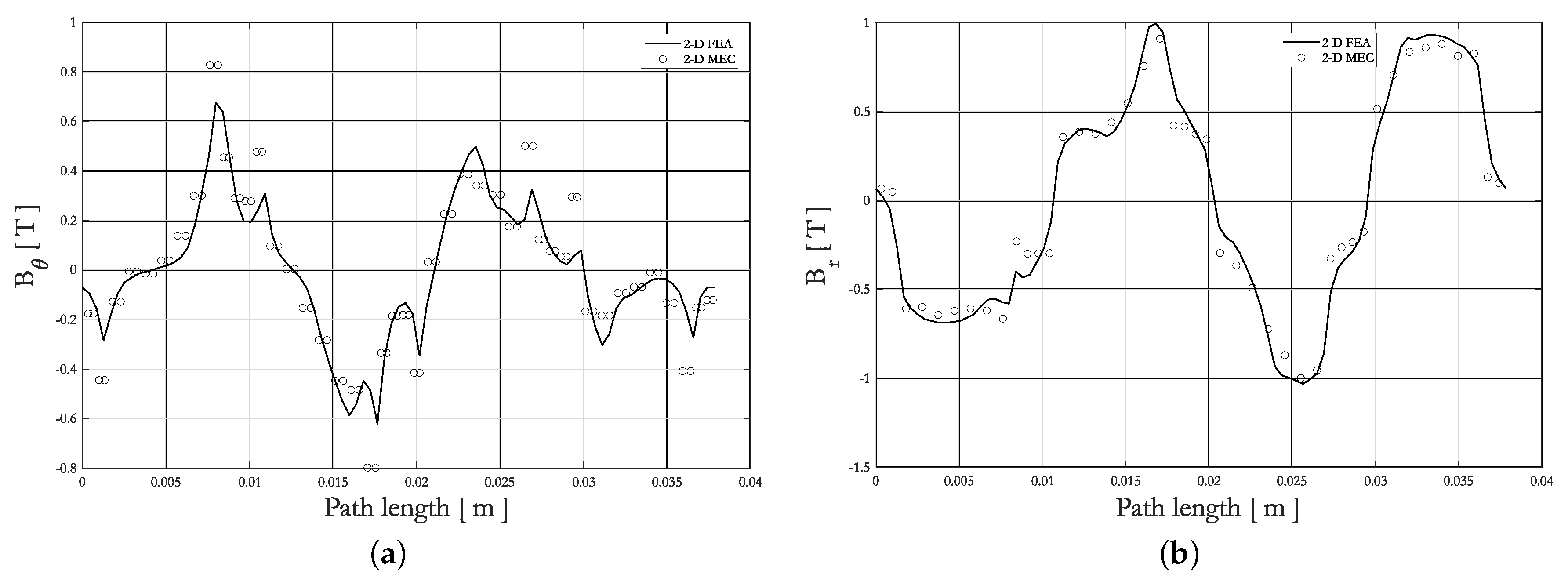
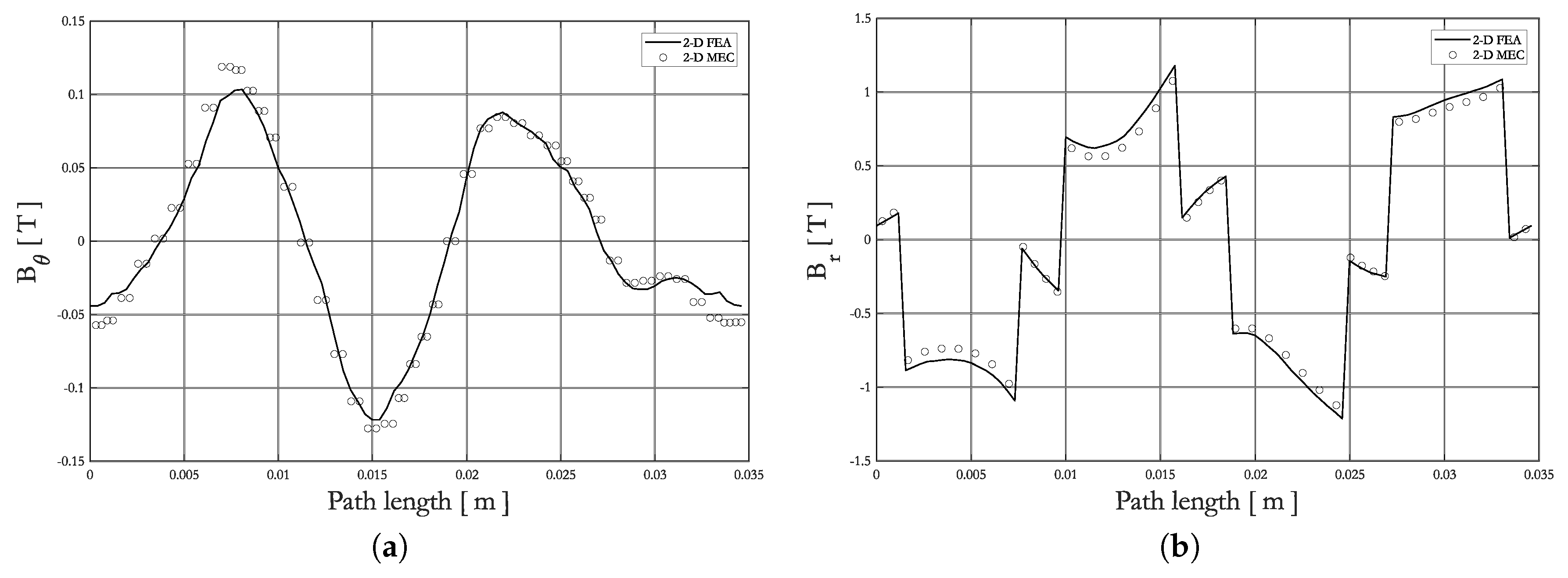
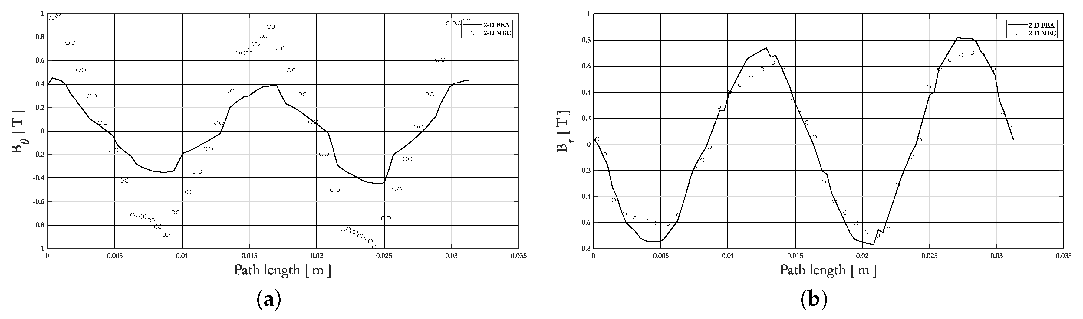
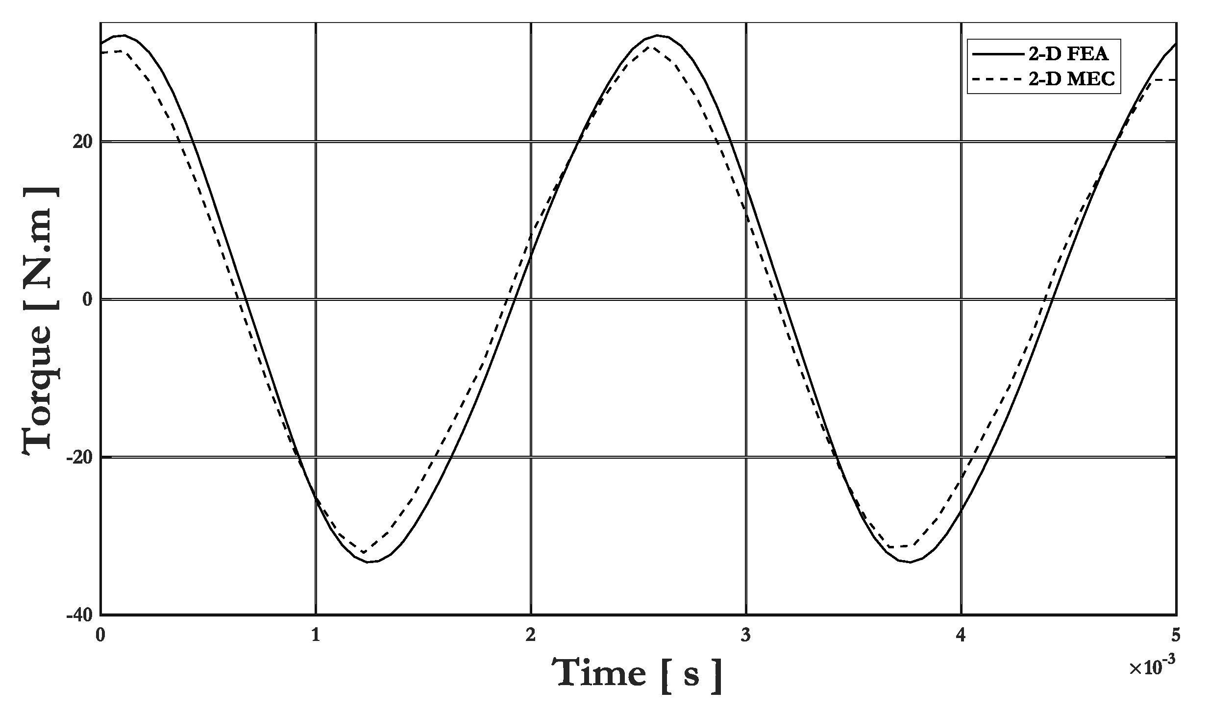
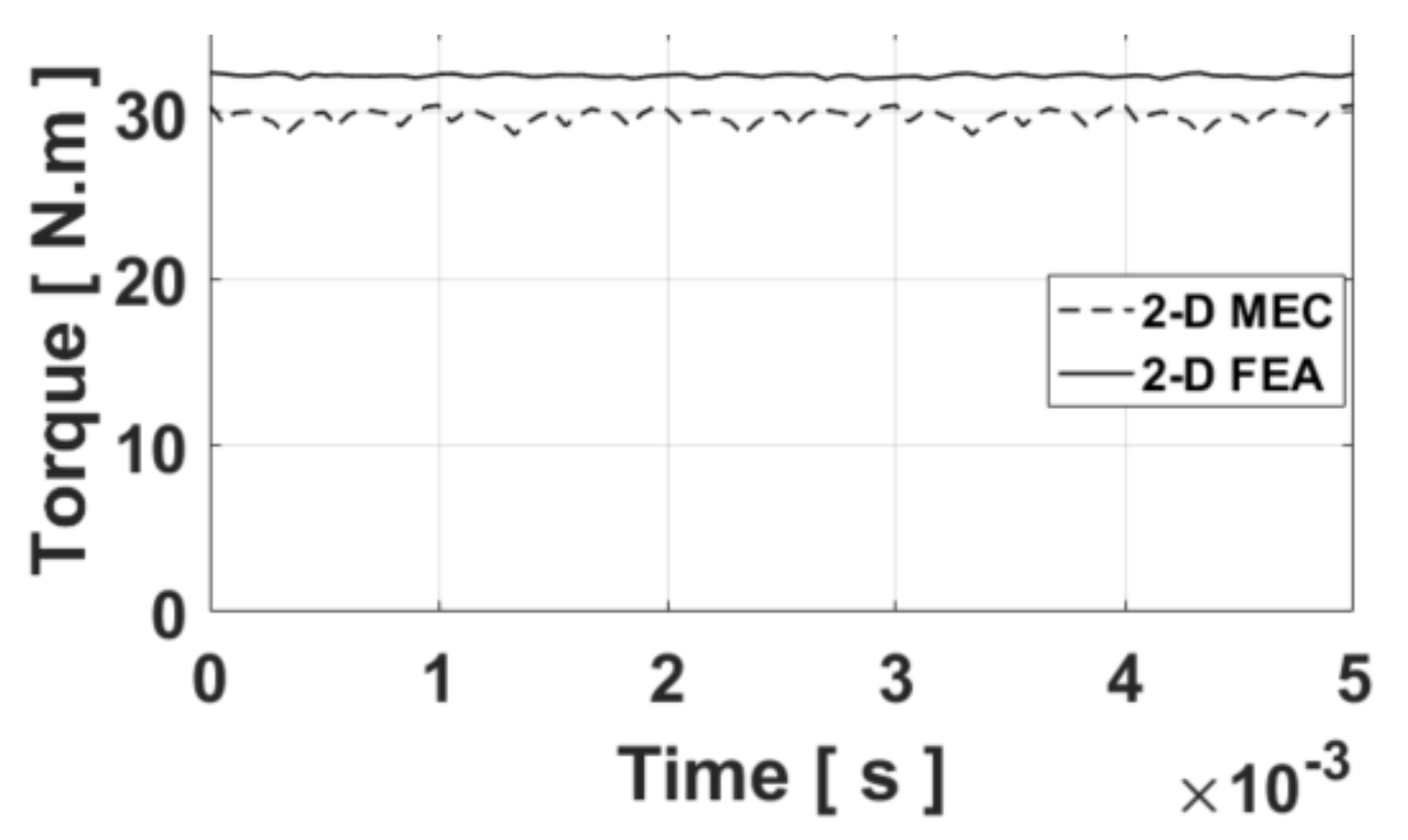
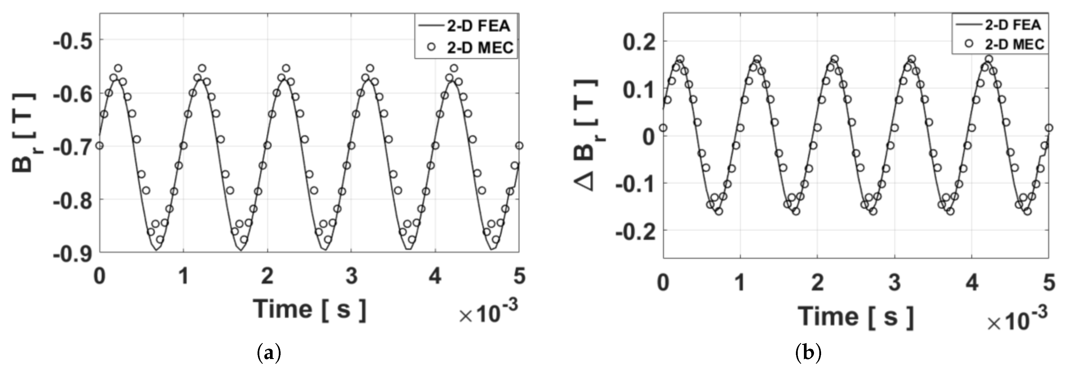
2.3. Validation of 2-D Generic MEC

The tangential and radial components of B at t = 0 s e c are given in Figure 7, Figure 8, Figure 9, Figure 10, Figure 11 and Figure 12 for the different path crossing, viz.: the stator yoke, stator teeth, stator air-gap, rotor air-gap, rotor PMs and rotor yoke. The components of B in the stator teeth [see Figure 8] are very saturated. The results are in agreement with 2-D nonlinear FEA, which confirms that the nonlinear solving method is accurate. The errors are due to the discretization of static and moving zones in both tangential and radial directions. For example, a sensibility study versus stator/rotor discretization on the computation time as well as on the iron losses determined from the magnetic flux density in the stator/rotor iron have been performed in [27]. The difference is mainly linked to the discretization for the rotor yoke where N d 3 r = 4 , which can be observed on the Figure 12a of the tangential component of B in the rotor yoke. The computation time is reduced by twice compared to the 2-D nonlinear FEA.
The simulation in time stepping leads to the results represented in Figure 13, Figure 14 and Figure 15. The electromagnetic torque evolution at locked rotor is given in Figure 13; this help us to find the shift angle to obtain the maximal electromagnetic torque at synchronism shown in Figure 14. The results give a decent satisfaction. The average electromagnetic torque given by 2-D nonlinear FEA is equal to 32 N m while the 2-D nonlinear adaptive MEC is slightly above 30 N m . The error is equal to 6.25 % . This small difference can be linked to the approach used to take into account the magnetic saturation, the rotor motion as well as the air-gap, stator and rotor discretization.
As mentioned in Section 2, the performed model will be used to extract the local physical quantities in PMs in order to estimate the eddy-current losses. Moreover, it should be noted that B θ in the PMs is considered negligible in relation to B r (see Figure 11). The losses are then determined from the normal magnetic field in the PMs. The model can give the waveform of B according to the time or the rotor position. The simulations are done for the path crossing the middle of PMs for one periodic pattern as shown in Figure 15a. The results are in agreement with the 2-D nonlinear FEA. Figure 15b gives the magnetic flux density evolution in the middle of North and South PMs.
Note that the average value of B is assumed to be not considered for the eddy-current loss calculation. The evolution of Δ B r for both middle of North and South PMs is shown in Figure 15b. It can be seen that the variation of B is practically identical. Thus, it can be concluded that the losses in North and South PMs are identical. Furthermore, only the results given for the South PM are given.

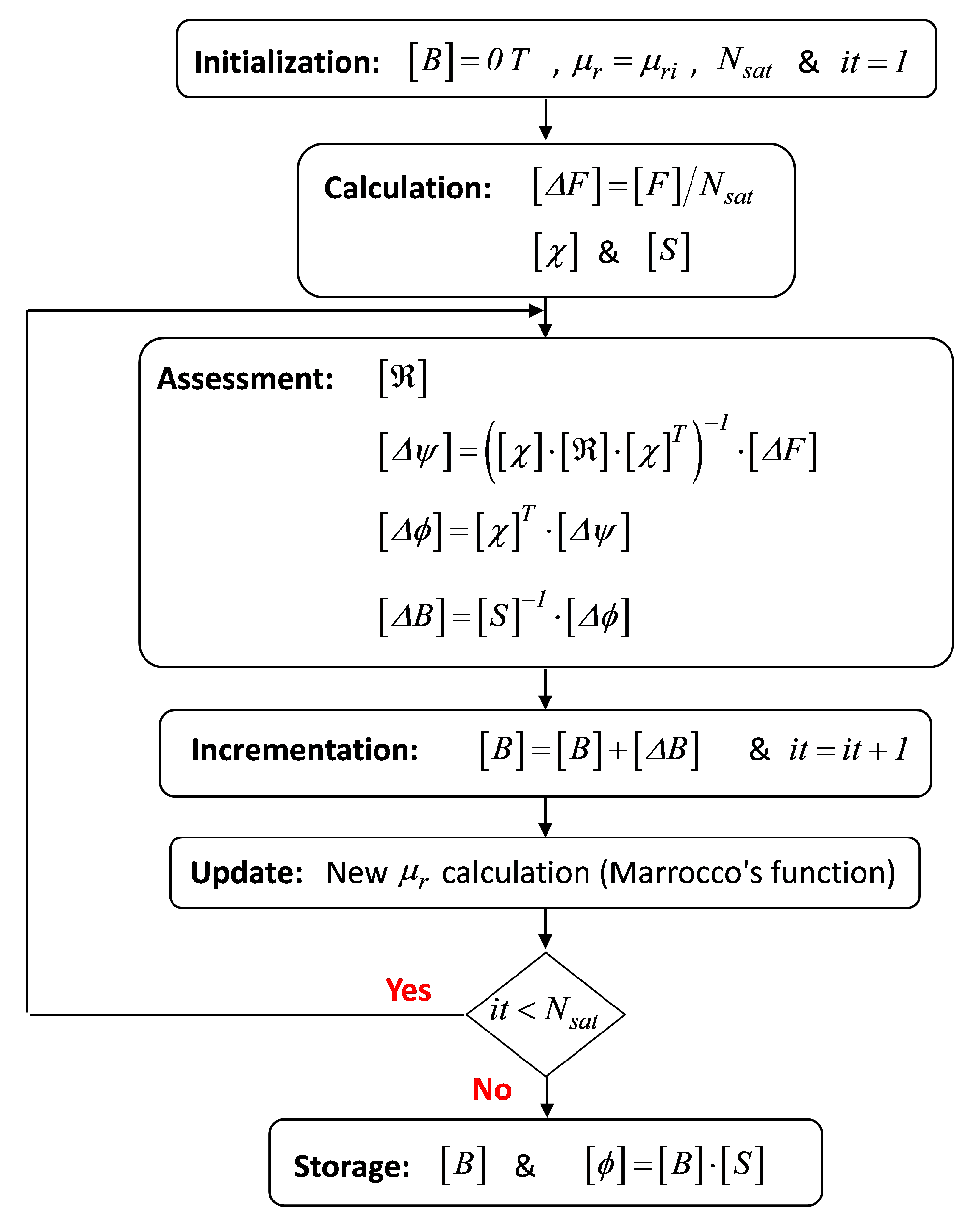
2.4. Formal Resolution of Maxwell’s Equations

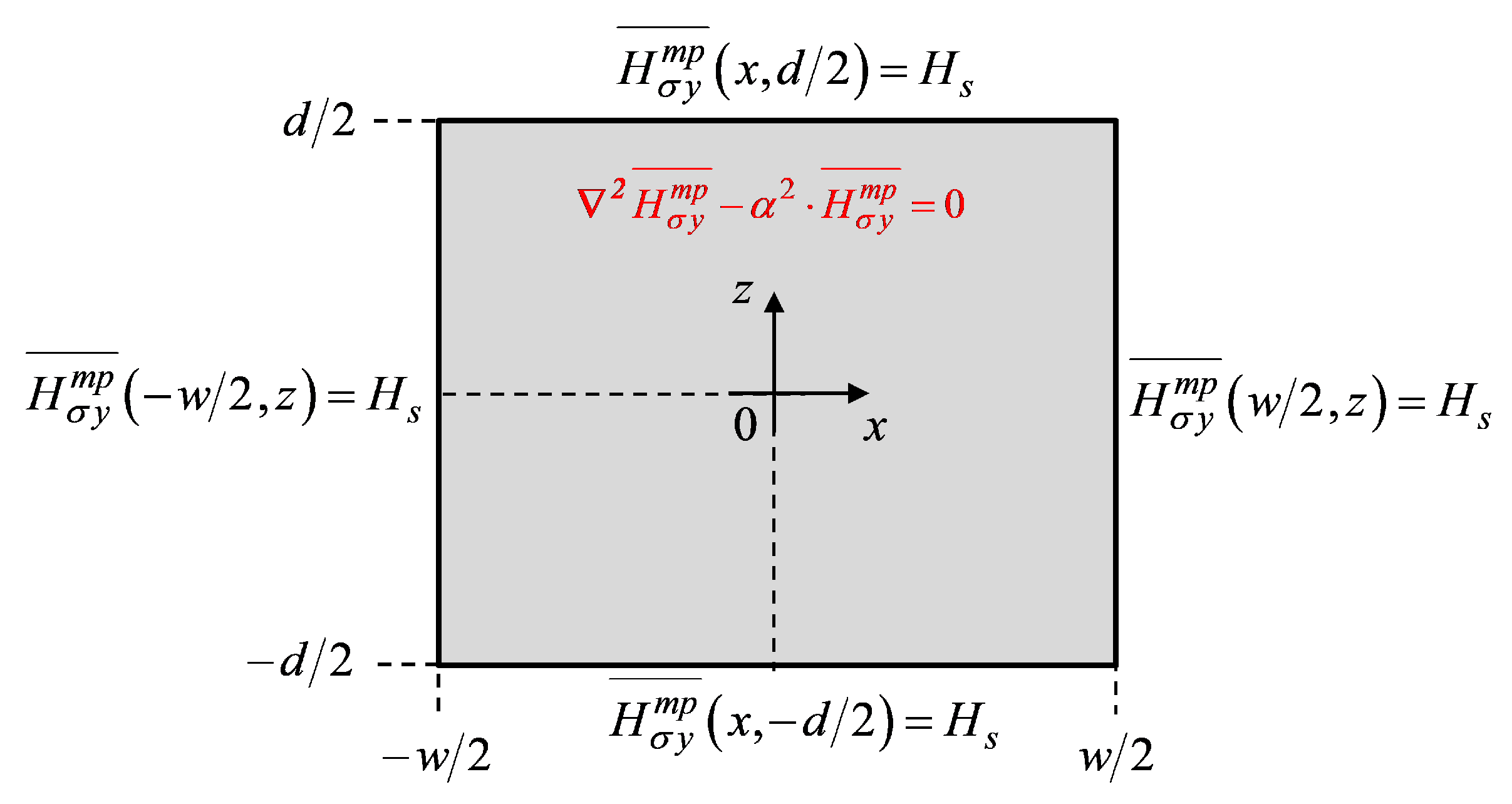
2.4.1. General Solution of Magnetic Field with the Skin Effect

The magnetic field with the skin is determined from an analytical model in 2-D Cartesian coordinates (i.e., the PMs are assumed rectangular) based on the Maxwell–Fourier method (i.e., the formal resolution of Maxwell’s equations by using the separation of variables method and the Fourier’s series). This permits to estimate the resultant eddy-current density in PMs in both directions (i.e., axial and circumferential axis). The BCs imposed on the 2-D analytical model are equivalent to the magnetic field obtained from the MEC. These BCs are considered homogeneous on the edges of massive conductive parts, which are equal to H s . This is a strong hypothesis because the magnetic field is naturally non-uniform. The value of magnetic field is defined as the normal magnetic field in the top or middle of PMs determined by 2-D generic MEC i.e., without the skin effect, viz., H s = B r ( 0 , 0 ) / μ m p . In our case, the model gives ability to use both conditions (i.e., in the top or middle of massive conductive parts), allowing to see the impact on the eddy-current loss calculation. Furthermore, the results will be given for different paths parallel to the tangential direction. The various BCs are shown in Figure 16.
In quasi-stationary approximation, inside a linear (non)magnetic material of electrical conductivity without electromagnetic sources, the partial differential equation in magnetodynamic in term of H m p can be defined by [28]
2 H mp μ m p · σ m p · H mp t = 0 ( Diffusion equation )
Using the complex notation, the magnetic field H mp = 0 ; H σ y m p ; 0 in massive conductive parts can be written as
H σ y m p = H σ y m p ¯ · e j ω t
where j = 1 and ω = 2 π f is the electrical pulse.
Therefore, (3) becomes in 2-D Cartesian coordinates the complex Helmholtz’s equation, viz.,
2 H σ y m p ¯ x 2 + 2 H σ y m p ¯ z 2 α 2 · H σ y m p ¯ = 0
where α 2 = j · μ m p · σ m p · ω .
By using the separation of variables method and by applying the BCs, the 2-D general solution of H σ y m p in both directions (i.e., x- and z-edges) can be written as Fourier’s series [28]
H σ y m p ¯ = H s · f σ ( x , z ) ¯ ,
f σ ( x , z ) ¯ = c h ( α · z ) c h α · d 2 + k = 1 , 3 , g k z ¯ · c h δ k · x cos λ k · z ,
g k z ¯ = e k z ¯ · s i n c λ k · d 2 c h δ k · w 2 with e k z ¯ = 2 1 λ k δ k 2 ,
where λ k = k π / d is the periodicity of H σ y m p ¯ in the z-axis, δ k = α 2 + λ k 2 , and k are the spatial harmonic orders.
It should be noted that H σ y m p is assumed to be invariant in the y-axis according to the study path. Moreover, when α = 0 (viz., σ m p = 0 S / m and f 0 + H z ) then f σ ( x , z ) ¯ = 1 thus giving H σ y m p ¯ = H s .

2.4.2. Eddy-Current Loss Formulation

The instantaneous density of power flow at a point is defined by the Poynting’s vector [28]
= E × H mp
Using J = σ · E = × H mp , this power across a closed surface, in terms of complex vectors, is given by the instantaneous apparent power
s a p p ¯ = s · d S = 1 σ m p · s J × H mp · d S = p + j · q
The real part of the surface integral of the complex Poynting’s vector gives the instantaneous ohmic losses and the imaginary part the instantaneous magnetic energy.
From BCs at edges of PMs (see Figure 16), the average of s a p p ¯ over an electrical cycle T = 2 π / ω can be defined by
S a p p ¯ = s a p p ¯ = h l σ m p · w / 2 w / 2 J x ¯ · H σ y m p ¯ * | z = d / 2 · d x d / 2 d / 2 J z ¯ · H σ y m p ¯ * | x = w / 2 · d z ,
where h l = h a / 2 · N d 2 r is the layers thickness in the r-axis of PMs with l the path number.
After development, (9) is then given by
S a p p ¯ = h l · H s 2 σ m p · w · α · s h α · d 2 c h α · d 2 + k = 1 , 3 , 2 δ k d · e k z ¯ λ k 2 · s h δ k · w 2 c h δ k · w 2 ,
S a p p ¯ = P + j · Q
It should be noted that P = { S a p p ¯ } represents the average eddy-current losses in PMs.

3. Approach of PM Eddy-Current Loss Calculation

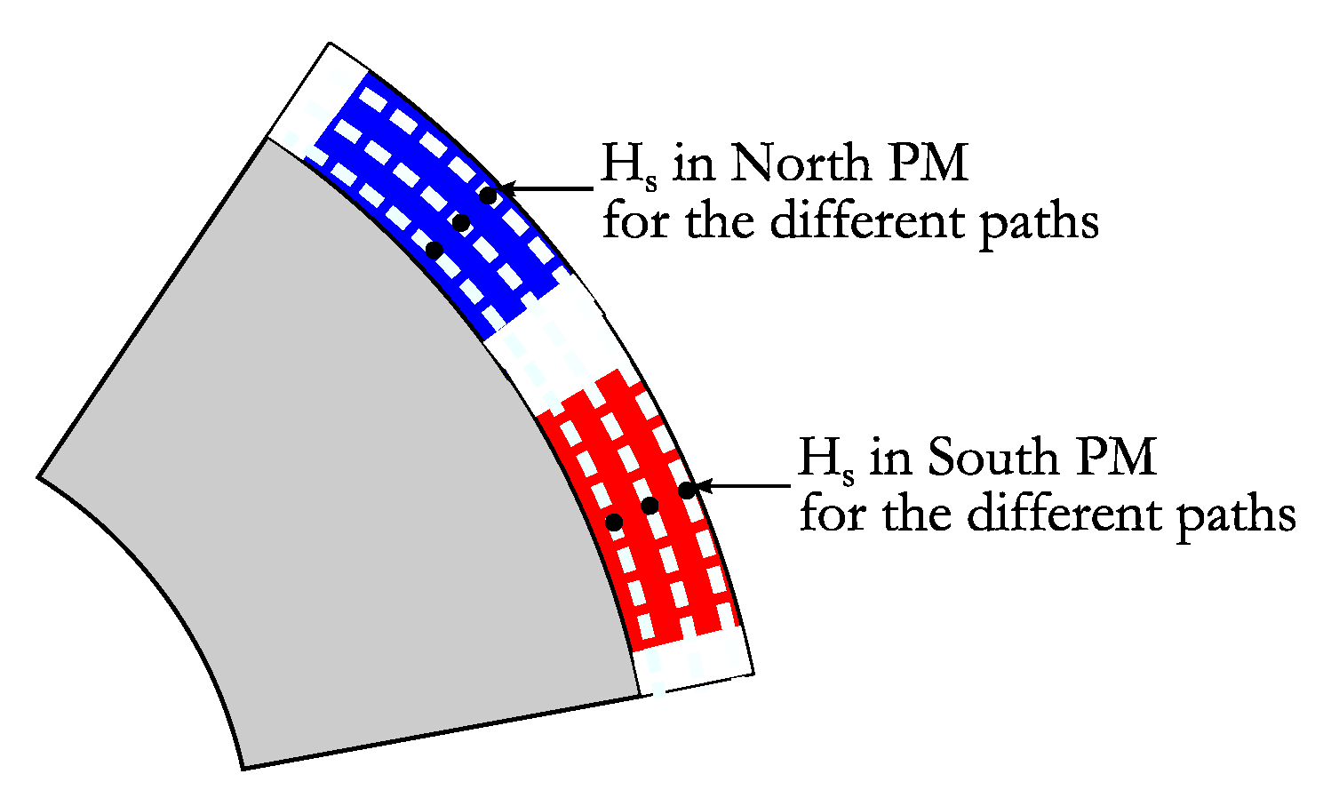
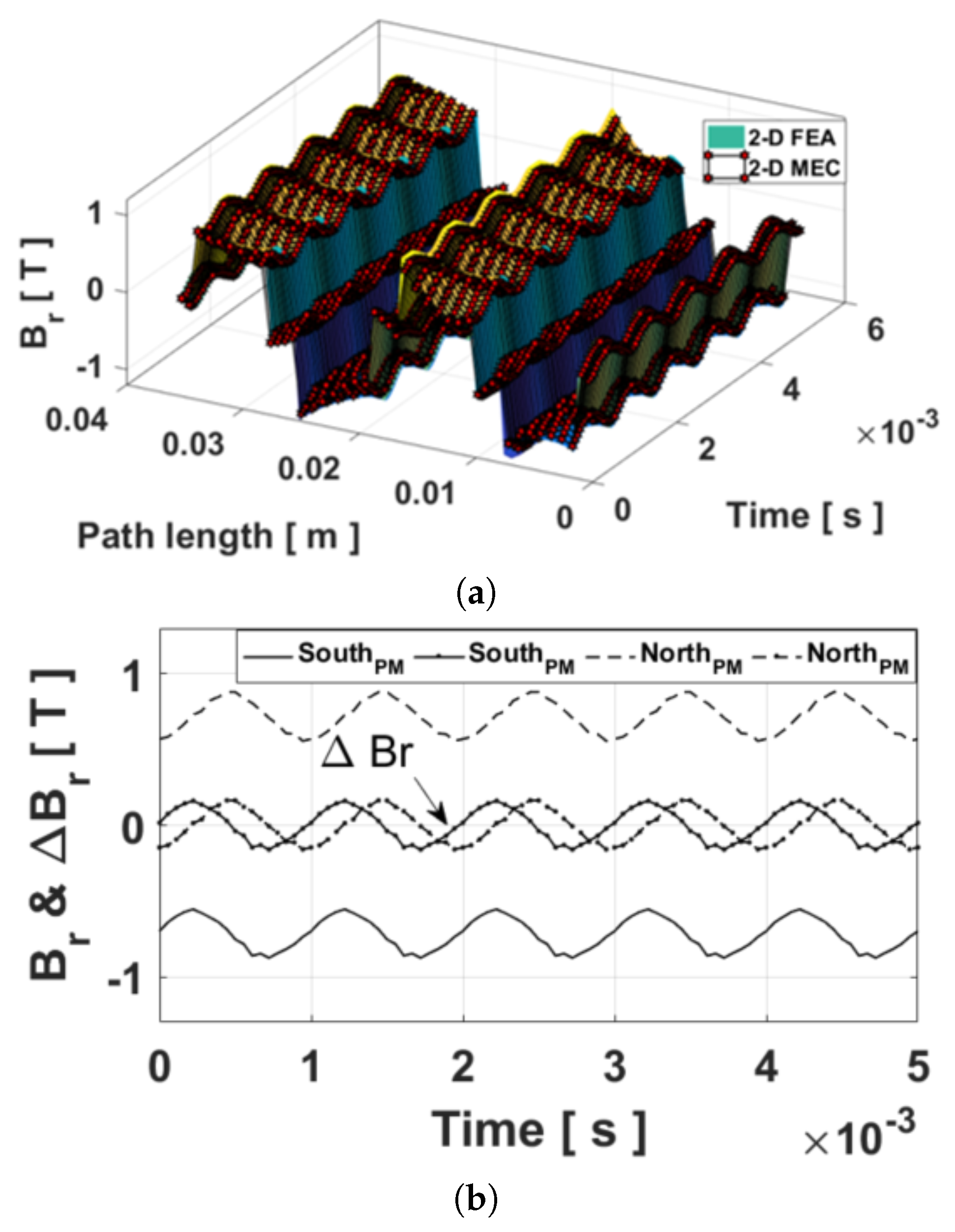
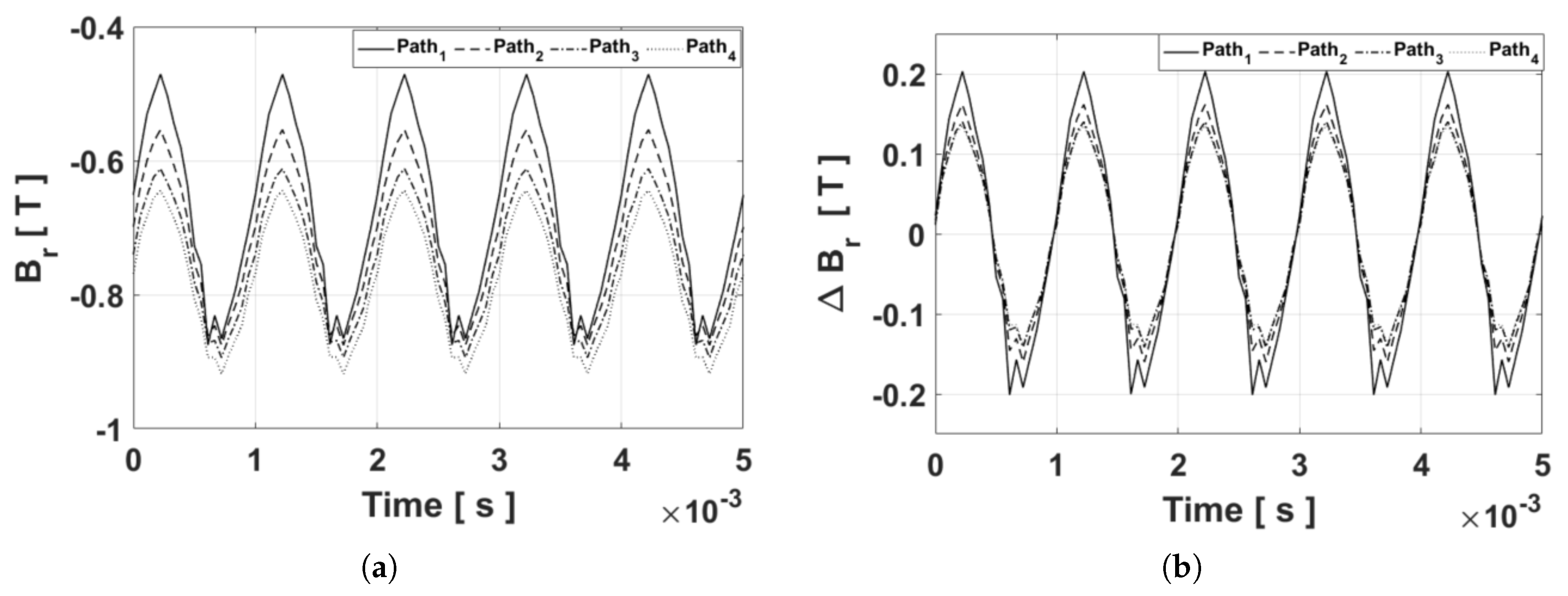
3.1. Magnetic Flux Density vs PM Thickness

Once the 2-D nonlinear adaptive MEC was validated on different stator and rotor paths. The radial component of B in the middle of North and South PMs according to the different tangential paths was evaluated. It should be noted that the paths number is imposed by the radial discretization number applied in the PMs region. The waveform of B in the PMs is done by stepwise simulation to get the radial component evolution according to the time or the rotor position.
Under the assumptions that the continuous magnitude B m of B σ y m p does not contribute to the eddy-current losses and that only the waveform Δ B r is subjected to the FFT. Hence, the most influential harmonics can be used to estimate the PMs eddy-current losses. Knowing that:
B σ y m p = B m + Δ B r
B σ y m p t = B m t + ( Δ B r ) t ( Δ B r ) t
Figure 17a provides the comparison between the developed model and 2-D FEA, for the radial component evolution in the middle of the North PM according to the time. The radial component variation for different path parallel to the tangential direction is illustrated on Figure 18a. Figure 17b presents the ripples in the middle of PMs. The validation is done by comparing the results to those of 2-D FEA. Figure 18b gives the ripples according to the symmetric axis of the PM, which are subjected to the FFT.

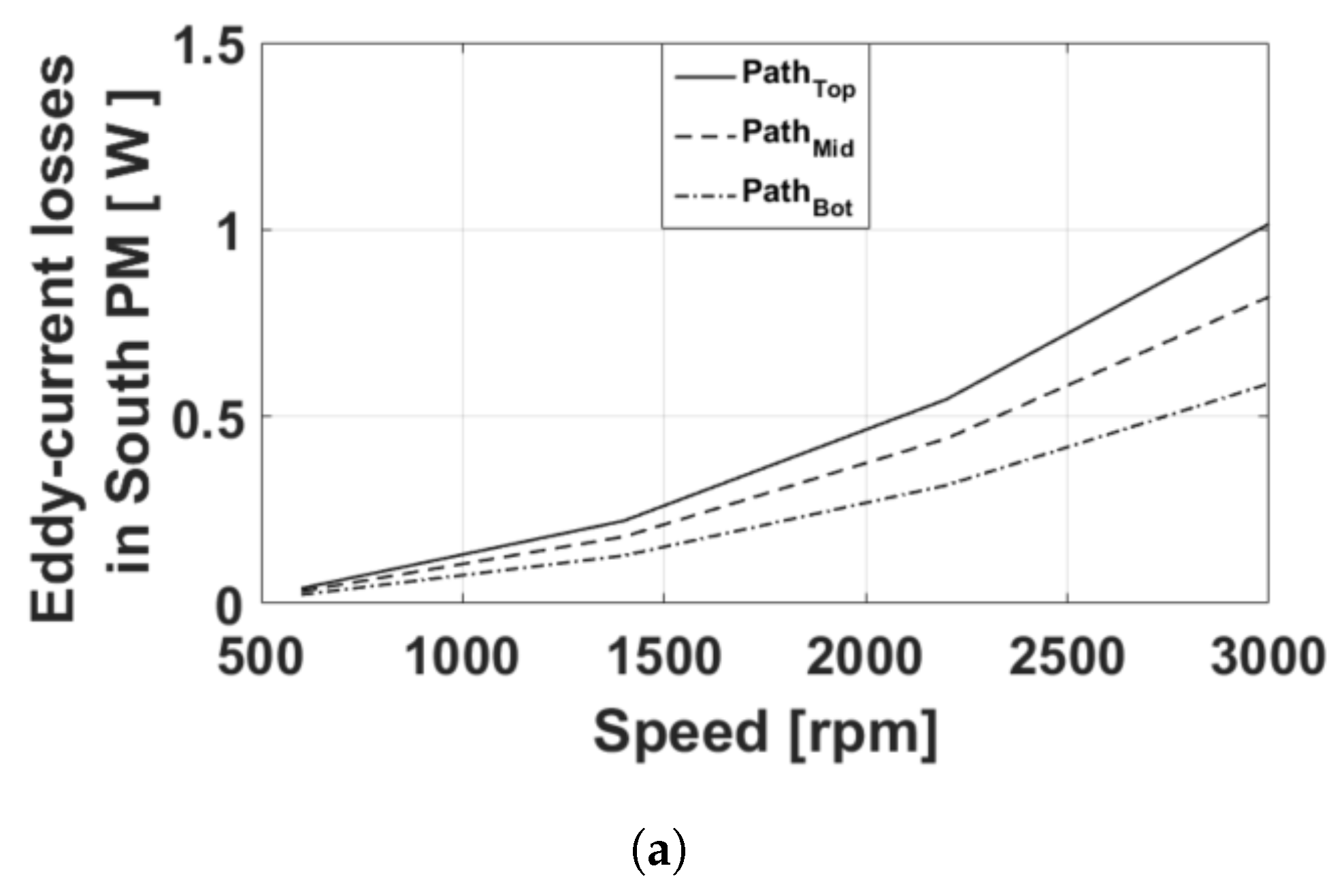
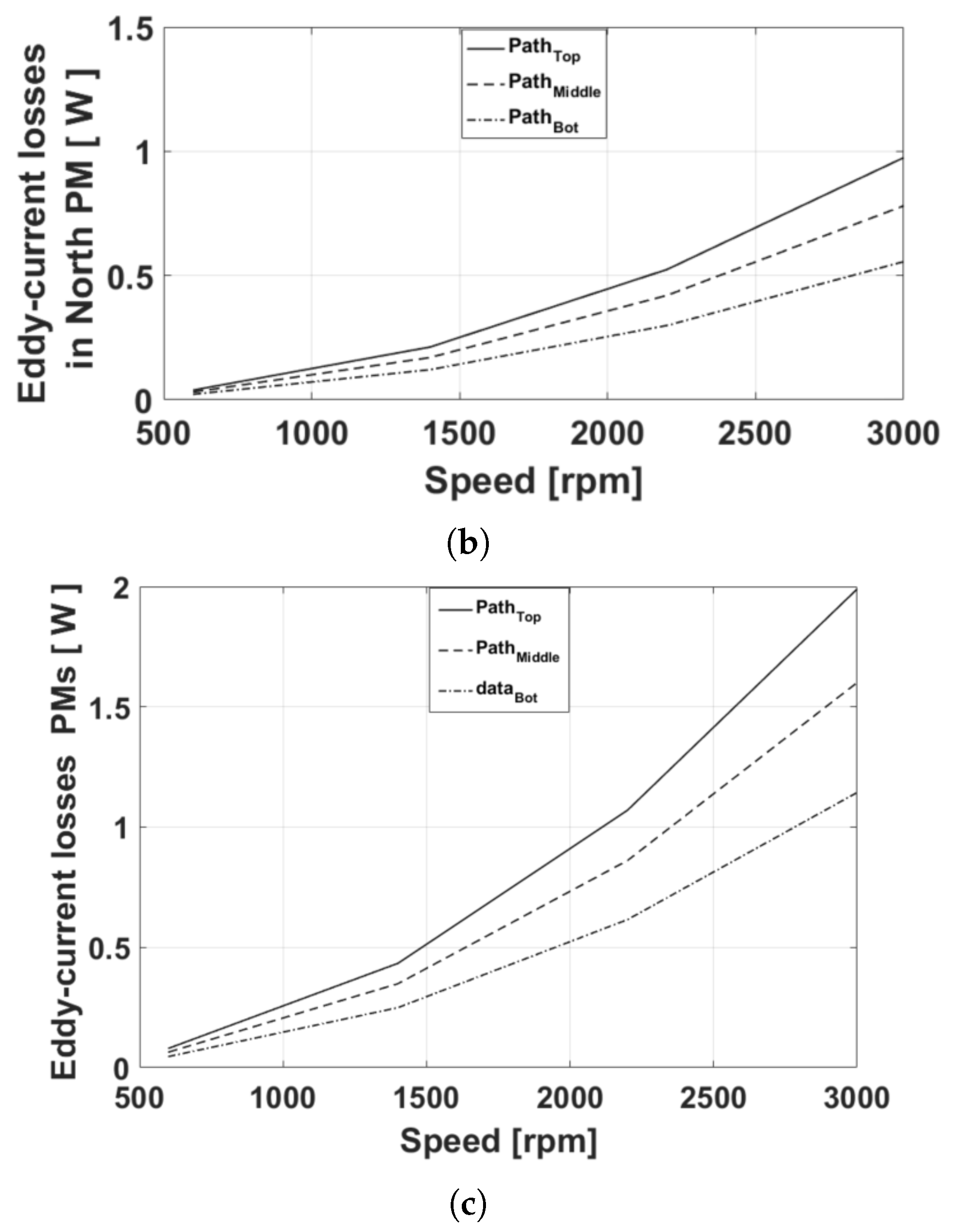
3.2. Eddy-Current Loss Evolution in Different Paths

Figure 19 and Figure 20 show the frequency spectrum of the radial component of B for different speeds. The spectral components are due to: (i) the supply (i.e., the current waveform), (ii) the slotting effect, and (iii) the spatial distribution of winding. Using the results given by the FFT for different paths in the PM, the PMs eddy-current losses can be estimated for each path as shown in Figure 21a,b.
By applying the sum, the total eddy-current losses due to the different paths are obtained as shown in Figure 21c. It should be noted that the eddy-current loss repartition in the PMs is greater at the top of PMs (whatever the PM magnetization) and decrease with to the PMs height to achieve the lower losses in the bottom of PMs. This distribution can be explained by the variation of the magnetic flux density amplitude that is more important in the region which is close to the air-gap, contrary to the bottom of PMs where the amplitude is relatively less important.

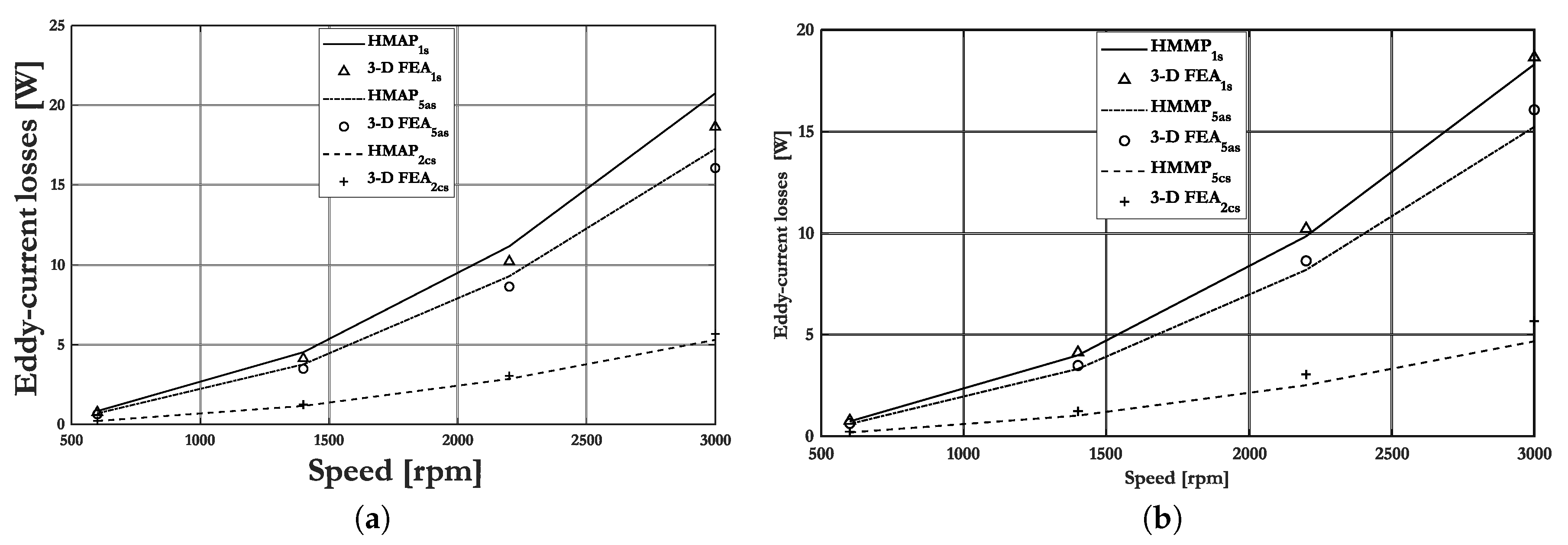
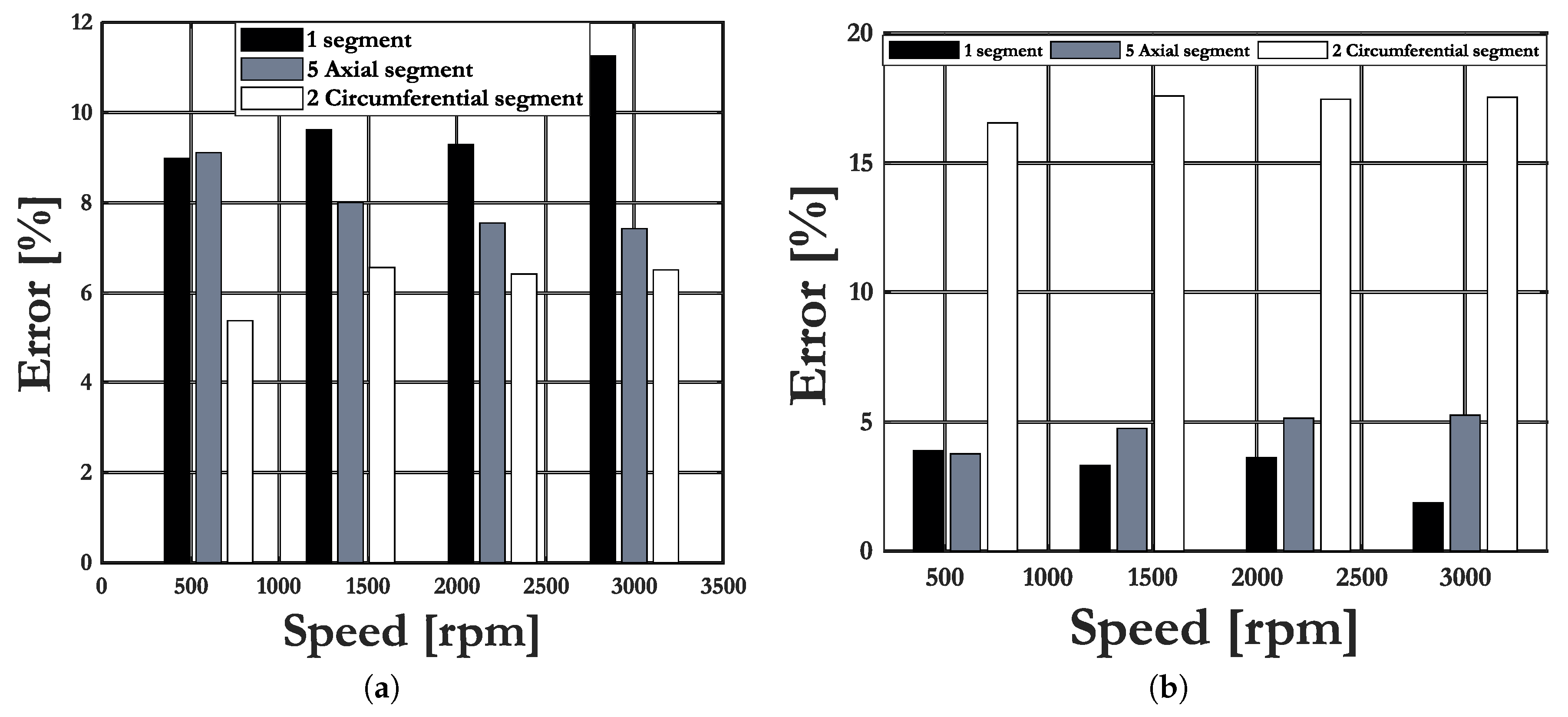
4. 3-D nonlinear FEA Validation With(out) PM Segmentation

In this section, the results of the hybrid multi-layer model are compared with those obtained by 3-D nonlinear FEA [21]. The PMs eddy-current losses were computed at different speed ranges for different segmentations as follow: (i) one segment (no segmentation), (ii) five axial segments, and (iii) two circumferential segments.
To prove the validation of this approach, the results are compared with those of 3-D nonlinear FEA in transient state [21]. Due to the boundary conditions (i.e., periodicity and Dirichlet conditions), the electrical machine can be reduced into 5-slots/4-poles. The mesh generation for 3-D nonlinear FEA is equal to 2,263,818 second order elements. It is given the eddy-current loss evolution in all PMs by using different segmentations with two different approaches (see Figure 22):
  • 1st approach: based on all paths;
  • 2nd approach: based on the middle path of PMs.
Figure 23 represents the relative error between each approach and 3-D nonlinear FEA. These errors are due to medium mesh in the 3-D nonlinear FEA as well as the magnetic field evaluation on all paths of the 2-D nonlinear adaptive MEC which is a data input the analytical model based on the Maxwell–Fourier method permitting the PM eddy-current loss calculation. In both cases, the results provide a good agreement with a maximal error of 16 % that is reached for the 2nd approach based on the middle path with two circumferential segments. While the maximal relative error for the 1st approach is estimated at 11 % , which is achieved for one segment (no-segmentation) at 3000 rpm.
The developed model returns both results based on to the two different approaches. It is better to use the 1st approach to estimate the eddy-current losses in the circumferential segmentation case.
Concerning the computation time, the 3-D nonlinear FEA takes 16 days for one simulation while the hybrid multi-layer model takes only 12 min. For an operating point, the computation time is then divided by 1920 with respect to 3-D nonlinear FEA.

5. Conclusions

In this work, a hybrid multi-layer model, combining a 2-D generic MEC with a 2-D analytical model based on the Maxwell–Fourier method was performed. This developed model was aimed to compute the volumic PM eddy-current losses in multi-phase PMSM. It is clearly seen that the PM eddy-current losses distribution present no-uniformity according to the PMs height. In this study case, these losses are greater at the top of PMs. This can be justified by the amplitude of the radial component of B, which is the highest in the top of PMs. Then, they decrease to achieve the minimal in the PM bottom. As a conclusion, the temperature repartition can be affected by the non-uniformity of the PM eddy-current loss distribution over the PM volume.

Author Contributions

Y.B. and D.O. prepared the structure and wrote the paper, F.D. and M.H. corrected and improved its content, F.D. and D.O. corrected the final version of the paper. All authors have read and agreed to the published version of the manuscript.

Acknowledgments

This work was supported by RENAULT-SAS, Guyancourt France. This scientific study is related to the project “Conception optimale des chaines de Traction Electrique” (COCTEL) financed by the “Agence De l’Environnement et de la Maîtrise de l’Énergie” (ADEME).

Conflicts of Interest

The authors declare no conflict of interest.

References

  1. Cassat, A.; Espanet, C.; Coleman, R.; Burdet, L.; Leleu, E.; Torregrossa, D.; M’Boua, J.; Miraoui, A. A practical solution to mitigate vibrations in industrial PM motors having concentric windings. IEEE Trans. Ind. Appl. 2012, 48, 1526–1538. [Google Scholar] [CrossRef]
  2. Levi, E. Multiphase Electric Machines for Variable-Speed Applications. IEEE Trans. Ind. Electron. 2008, 55, 1893–1909. [Google Scholar] [CrossRef]
  3. Scuiller, F.; Charpentier, J.F.; Semail, E.; Clenet, S. Comparison of two 5-phase permanent magnet machine winding configurations. Application on naval propulsion specifications. In Proceedings of the 2007 IEEE International Electric Machines & Drives Conference, Antalya, Turkey, 3–5 May 2007; Volume 1, pp. 34–39. [Google Scholar] [CrossRef]
  4. de la Barriere, O.; Hlioui, S.; Ben Ahmed, H.; Gabsi, M. An Analytical Model for the Computation of No-Load Eddy-Current Losses in the Rotor of a Permanent Magnet Synchronous Machine. IEEE Trans. Magn. 2016, 52, 1–13. [Google Scholar] [CrossRef] [Green Version]
  5. Dubas, F.; Espanet, C. Semi-Analytical Solution of 2-D Rotor Eddy-Current Losses due to the Slotting Effect in SMPMM. In Proceedings of the 17th Conference on the Computation of Electromagnetic Fields COMPUMAG 2009, Florianopolis, Brasil, 22–26 November 2009; pp. 20–25. [Google Scholar]
  6. Markovic, M.; Perriard, Y. A simplified determination of the permanent magnet (PM) eddy current losses due to slotting in a PM rotating motor. In Proceedings of the 2008 International Conference on Electrical Machines and Systems (ICEMS), Wuhan, China, 17–20 October 2008; pp. 309–313. [Google Scholar]
  7. Dubas, F.; Espanet, C.; Miraoui, A. Field Diffusion Equation in High-Speed Surface-Mounted Permanent Magnet Motors, Parasitic Eddy-Current Losses. In Proceedings of the 6th International Symposium on Advanced Electromechanical Motion Systems, Lausanne, Switzerland, 27–29 September 2005; pp. 1–6. [Google Scholar]
  8. Deng, F.; Nehl, T. Analytical modeling of eddy-current losses caused by pulse-width-modulation switching in permanent-magnet brushless direct-current motors. IEEE Trans. Magn. 1998, 34, 3728–3736. [Google Scholar] [CrossRef]
  9. Nuscheler, R. Two-dimensional analytical model for eddy-current rotor loss calculation of PMS machines with concentrated stator windings and a conductive shield for the magnets. In Proceedings of the XIX International Conference on Electrical Machines (ICEM 2010), Rome, Italy, 6–8 September 2010; pp. 1–6. [Google Scholar] [CrossRef]
  10. Mirzaei, M.; Binder, A.; Funieru, B.; Susic, M. Analytical Calculations of Induced Eddy Currents Losses in the Magnets of Surface Mounted PM Machines With Consideration of Circumferential and Axial Segmentation Effects. IEEE Trans. Magn. 2012, 48, 4831–4841. [Google Scholar] [CrossRef]
  11. Yoshida, K.; Hita, Y.; Kesamaru, K. Eddy-current loss analysis in PM of surface-mounted-PM SM for electric vehicles. IEEE Trans. Magn. 2000, 36, 1941–1944. [Google Scholar] [CrossRef]
  12. El-Hasan, T. Rotor eddy current determination using finite element analysis for High-Speed Permanent Magnet Machines. In Proceedings of the 2014 IEEE 23rd International Symposium on Industrial Electronics (ISIE), Istanbul, Turkey, 1–4 June 2014; pp. 885–889. [Google Scholar] [CrossRef]
  13. Saban, D.M.; Lipo, T.A. Hybrid Approach for Determining Eddy-Current Losses in High-Speed PM Rotors. In Proceedings of the 2007 IEEE International Electric Machines & Drives Conference, Antalya, Turkey, 3–5 May 2007; Volume 1, pp. 658–661. [Google Scholar] [CrossRef]
  14. Gerlach, T.; Rabenstein, L.; Dietz, A.; Kremser, A.; Gerling, D. Determination of eddy current losses in permanent magnets of SPMSM with concentrated windings: A hybrid loss calculation method and experimental verification. In Proceedings of the 2018 Thirteenth International Conference on Ecological Vehicles and Renewable Energies (EVER), Monte-Carlo, Monaco, 10–12 April 2018; pp. 1–8. [Google Scholar] [CrossRef]
  15. Dubas, F.; Rahideh, A. Two-Dimensional Analytical Permanent-Magnet Eddy-Current Loss Calculations in Slotless PMSM Equipped With Surface-Inset Magnets. IEEE Trans. Magn. 2014, 50, 54–73. [Google Scholar] [CrossRef]
  16. Ouamara, D.; Dubas, F. Permanent-Magnet Eddy-Current Losses: A Global Revision of Calculation and Analysis. Math. Comput. Appl. 2019, 24, 67. [Google Scholar] [CrossRef] [Green Version]
  17. Pfister, P.D.; Yin, X.; Fang, Y. Slotted Permanent-Magnet Machines: General Analytical Model of Magnetic Fields, Torque, Eddy Currents, and Permanent-Magnet Power Losses Including the Diffusion Effect. IEEE Trans. Magn. 2016, 52, 1–13. [Google Scholar] [CrossRef]
  18. Benlamine, R.; Dubas, F.; Randi, S.A.; Lhotellier, D.; Espanet, C. 3-D Numerical Hybrid Method for PM Eddy-Current Losses Calculation: Application to Axial-Flux PMSMs. IEEE Trans. Magn. 2015, 51, 1–10. [Google Scholar] [CrossRef] [Green Version]
  19. Masmoudi, A.; Masmoudi, A. 3-D Analytical Model With the End Effect Dedicated to the Prediction of PM Eddy-Current Loss in FSPMMs. IEEE Trans. Magn. 2015, 51, 1–11. [Google Scholar] [CrossRef]
  20. Ouamara, D.; Dubas, F.; Randi, S.A.; Benallal, M.N.; Espanet, C. Optimal Design of Multi-phases Permanent-Magnet Synchronous Machines Using Genetic Algorithms. Mediterr. J. Model. Simul. 2018, 10, 29–44. [Google Scholar]
  21. Altair Flux. Electromagnetic, Electric, and Thermal Analysis. Available online: https://www.altair.com/flux/ (accessed on 4 March 2020).
  22. Dubas, F.; Benlamine, R.; Randi, S.A.; Lhotellier, D.; Espanet, C. 2-D or quasi 3-D nonlinear adaptative magnetic equivalent circuit, Part I: Generalized modeling with air-gap sliding-line technic. Appl. Energy. under review.
  23. Benlamine, R.; Dubas, F.; Randi, S.A.; Lhotellier, D.; Espanet, C. 2-D or quasi 3-D nonlinear adaptive magnetic equivalent circuit, Part II: Application to axial-flux interior permanent-magnet synchronous machines. Appl. Energy. under review.
  24. Benlamine, R.; Dubas, F.; Randi, S.A.; Lhotellier, D.; Espanet, C. Modeling of an axial-flux interior PMs machine for an automotive application using magnetic equivalent circuit. In Proceedings of the 2015 18th International Conference on Electrical Machines and Systems (ICEMS), Pattaya, Thailand, 25–28 October 2015; pp. 1266–1271. [Google Scholar] [CrossRef]
  25. Benlamine, R.; Hamiti, T.; Vangraefschepe, F.; Dubas, F.; Lhotellier, D. Modeling of a coaxial magnetic gear equipped with surface mounted PMs using nonlinear adaptive magnetic equivalent circuits. In Proceedings of the 2016 XXII International Conference on Electrical Machines (ICEM), Lausanne, Switzerland, 4–7 September 2016; pp. 1888–1894. [Google Scholar] [CrossRef] [Green Version]
  26. Benlamine, R.; Benmessaoud, Y.; Dubas, F.; Espanet, C. Nonlinear Adaptive Magnetic Equivalent Circuit of a Radial-Flux Interior Permanent-Magnet Machine Using Air-Gap Sliding-Line Technic. In Proceedings of the 2017 IEEE Vehicle Power and Propulsion Conference (VPPC), Belfort, France, 11–14 December 2017; Volume 24, pp. 1–6. [Google Scholar] [CrossRef] [Green Version]
  27. Utegenova, S.; Dubas, F.; Jamot, M.; Glises, R.; Truffart, B.; Mariotto, D.; Lagonotte, P.; Desevaux, P. An Investigation into the Coupling of Magnetic and Thermal Analysis for a Wound-Rotor Synchronous Machine. IEEE Trans. Ind. Electron. 2018, 65, 3406–3416. [Google Scholar] [CrossRef]
  28. Stoll, R.L. The Analysis of Eddy Currents; Clarendon Press: Oxford, UK, 1974. [Google Scholar]
Figure 1. General flowchart of hybrid multi-layer model.
Mca 25 00014 g001
Figure 2. Description of the machine: Topology and winding distribution.
Mca 25 00014 g002
Figure 3. Tangential parallel paths in PMs.
Mca 25 00014 g003
Figure 4. Mesh element discretization [22].
Mca 25 00014 g004
Figure 5. Components of mesh elements [22].
Mca 25 00014 g005
Figure 6. Flowchart of the iterative solving of the nonlinear system [22].
Mca 25 00014 g006
Figure 7. Waveform of B in the stator yoke: (a) tangential, and (b) radial component.
Mca 25 00014 g007
Figure 8. Waveform of B in the stator teeth: (a) tangential, and (b) radial component.
Mca 25 00014 g008
Figure 9. Waveform of B in the stator air-gap: (a) tangential, and (b) radial component.
Mca 25 00014 g009
Figure 10. Waveform of B in the rotor air-gap: (a) tangential, and (b) radial component.
Mca 25 00014 g010
Figure 11. Waveform of B in the rotor PMs: (a) tangential, and (b) radial component.
Mca 25 00014 g011
Figure 12. Waveform of B in the rotor yoke: (a) tangential, and (b) radial component.
Mca 25 00014 g012
Figure 13. Electromagnetic torque at locked rotor.
Mca 25 00014 g013
Figure 14. Electromagnetic torque at synchronism.
Mca 25 00014 g014
Figure 15. Evolution of B: (a) versus time for the path crossing the middle of PMs, and (b) in the middle of North and South PMs with(out) the average value.
Mca 25 00014 g015
Figure 16. BCs at edges of PMs in ( x , z ) coordinate system.
Mca 25 00014 g016
Figure 17. Validation of the radial component of B in the middle of the North PM: (a) with and (b) without average value.
Mca 25 00014 g017
Figure 18. Evolution of the radial component of B in the middle of the North PM according to the time for different tangential path: (a) with and (b) without the average value.
Mca 25 00014 g018
Figure 19. The frequency spectrum of the radial component of B in the middle of the North PM at 600 rpm.
Mca 25 00014 g019
Figure 20. The frequency spectrum of the radial component of B in the middle of the North PM at 3000 rpm.
Mca 25 00014 g020
Figure 21. Non-uniform volume repartition of the eddy current losses vs. speed for different paths: (a) South PMs, (b) North PMs, and (c) Total.
Mca 25 00014 g021aMca 25 00014 g021b
Figure 22. Eddy-current losses comparison with 3-D FEA: (a) all paths, and (b) middle path of PMs.
Mca 25 00014 g022
Figure 23. Relative error between the hybrid model and 3-D FEA: (a) all paths, and (b) middle path of PMs.
Mca 25 00014 g023
Table 1. Geometrical data of the machine [20].
DesignationSymbolValueUnit
Slots number Q s 20-
Phases numberm5-
Poles number 2 p 16-
Slot-opening/tooth-pitch α s o 60%
Isthmus-opening/slot α i s 53%
PM pole-arc/pole-pitch α a 72%
Winding-opening/slot α w 92%
Stator bore diameter D e 49.4 mm
External diameter D e s 65.7 mm
Internal diameter D i 34.9 mm
Stator yoke height h c s 3mm
Rotor yoke height h c r 3mm
PM height h a 2.5 mm
Tooth height h d 4.8 mm
Machine length l m 100mm
Table 2. Physical data of the machine.
DesignationSymbolValueUnit
SpeedN3000rpm
Electromagnetic torque T e m 30Nm
CurrentI30A
Table 3. Discretization number.
Discretization/ZonesStatorRotor
Tangential [ 2 1 7 1 2 ] [ 2 7 2 ]
Radial [ 1 2 3 2 3 ] [ 3 6 4 1 ]

