Abstract
We provide easy and readable GNU Octave/MATLAB code for the simulation of mathematical models described by ordinary differential equations and for the solution of optimal control problems through Pontryagin’s maximum principle. For that, we consider a normalized HIV/AIDS transmission dynamics model based on the one proposed in our recent contribution (Silva, C.J.; Torres, D.F.M. A SICA compartmental model in epidemiology with application to HIV/AIDS in Cape Verde. Ecol. Complex. 2017, 30, 70–75), given by a system of four ordinary differential equations. An HIV initial value problem is solved numerically using the ode45 GNU Octave function and three standard methods implemented by us in Octave/MATLAB: Euler method and second-order and fourth-order Runge–Kutta methods. Afterwards, a control function is introduced into the normalized HIV model and an optimal control problem is formulated, where the goal is to find the optimal HIV prevention strategy that maximizes the fraction of uninfected HIV individuals with the least HIV new infections and cost associated with the control measures. The optimal control problem is characterized analytically using the Pontryagin Maximum Principle, and the extremals are computed numerically by implementing a forward-backward fourth-order Runge–Kutta method. Complete algorithms, for both uncontrolled initial value and optimal control problems, developed under the free GNU Octave software and compatible with MATLAB are provided along the article.
Keywords:
numerical algorithms; optimal control; HIV/AIDS model; GNU Octave; open source code for optimal control through Pontryagin Maximum Principle MSC:
34K28; 49N90; 92D30
1. Introduction
In recent years, mathematical modeling of processes in biology and medicine, in particular in epidemiology, has led to significant scientific advances both in mathematics and biosciences [1,2]. Applications of mathematics in biology are completely opening new pathways of interactions, and this is certainly true in the area of optimal control: a branch of applied mathematics that deals with finding control laws for dynamical systems over a period of time such that an objective functional is optimized [3,4]. It has numerous applications in both biology and medicine [5,6,7,8].
To find the best possible control for taking a dynamical system from one state to another, one uses, in optimal control theory, the celebrated Pontryagin’s maximum principle (PMP), formulated in 1956 by the Russian mathematician Lev Pontryagin and his collaborators [3]. Roughly speaking, PMP states that it is necessary for any optimal control along with the optimal state trajectory to satisfy the so-called Hamiltonian system, which is a two-point boundary value problem, plus a maximality condition on the Hamiltonian. Although a classical result, PMP is usually not taught to biologists and mathematicians working on mathematical biology. Here, we show how such scientists can easily implement the necessary optimality conditions given by the PMP, numerically, and can benefit from the power of optimal control theory. For that, we consider a mathematical model for HIV.
HIV modeling and optimal control is a subject under strong current research: see, e.g., Reference [9] and the references therein. Here, we consider the SICA epidemic model for HIV transmission proposed in References [10,11], formulate an optimal control problem with the goal to find the optimal HIV prevention strategy that maximizes the fraction of uninfected HIV individuals with least HIV new infections and cost associated with the control measures, and give complete algorithms in GNU Octave to solve the considered problems. We trust that our work, by providing the algorithms in an open programming language, contributes to reducing the so-called “replication crisis” (an ongoing methodological crisis in which it has been found that many scientific studies are difficult or impossible to replicate or reproduce [12]) in the area of optimal biomedical research. We trust our current work will be very useful to a practitioner from the disease control area and will become a reference in the field of epidemiology for those interested to include an optimal control component in their work.
2. A Normalized SICA HIV/AIDS Model
We consider the SICA epidemic model for HIV transmission proposed in References [10,11], which is given by the following system of ordinary differential equations:
The model in Equation (1) subdivides human population into four mutually exclusive compartments: susceptible individuals (S); HIV-infected individuals with no clinical symptoms of AIDS (the virus is living or developing in the individuals but without producing symptoms or only mild ones) but able to transmit HIV to other individuals (I); HIV-infected individuals under ART treatment (the so-called chronic stage) with a viral load remaining low (C); and HIV-infected individuals with AIDS clinical symptoms (A). The total population at time t, denoted by , is given by . Effective contact with people infected with HIV is at a rate , given by
where is the effective contact rate for HIV transmission. The modification parameter accounts for the relative infectiousness of individuals with AIDS symptoms in comparison to those infected with HIV with no AIDS symptoms (individuals with AIDS symptoms are more infectious than HIV-infected individuals—pre-AIDS). On the other hand, translates the partial restoration of immune function of individuals with HIV infection that use ART correctly [10]. All individuals suffer from natural death at a constant rate . Both HIV-infected individuals with and without AIDS symptoms have access to ART treatment: HIV-infected individuals with no AIDS symptoms I progress to the class of individuals with HIV infection under ART treatment C at a rate , and HIV-infected individuals with AIDS symptoms are treated for HIV at rate . An HIV-infected individual with AIDS symptoms A that starts treatment moves to the class of HIV-infected individuals I and after, if the treatment is maintained, will be transferred to the chronic class C. Individuals in the class C leave to the class I at a rate due to a default treatment. HIV-infected individuals with no AIDS symptoms I that do not take ART treatment progress to the AIDS class A at rate . Finally, HIV-infected individuals with AIDS symptoms A suffer from an AIDS-induced death at a rate d.
In the situation where the total population size is not constant, it is often convenient to consider the proportions of each compartment of individuals in the population, namely
The state variables s, i, c, and a satisfy the following system of differential equations:
with for all .
3. Numerical Solution of the SICA HIV/AIDS Model
In this section, we consider Equation (2) subject to the initial conditions given by
by the fixed parameter values from Table 1, and by the final time value of (years).

Table 1.
Parameter values of the HIV/AIDS model in Equation (2) taken from Reference [11] and references cited therein.
All our algorithms, developed to solve numerically the initial value problems in Equations (2) and (3), are developed under the free GNU Octave software (version 5.1.0), a high-level programming language primarily intended for numerical computations and is the major free and mostly compatible alternative to MATLAB [13]. We implement three standard basic numerical techniques: Euler, second-order Runge–Kutta, and fourth-order Runge–Kutta. We compare the obtained solutions with the one obtained using the ode45 GNU Octave function.
3.1. Default ode45 Routine of GNU Octave
Using the provided ode45 function of GNU Octave, which solves a set of non-stiff ordinary differential equations with the well known explicit Dormand–Prince method of order 4, one can solve the initial value problems in Equations (2) and (3) as follows:
- function dy = odeHIVsystem(t,y)% Parameters of the modelmi = 1.0 / 69.54; b = 2.1 * mi; beta = 1.6;etaC = 0.015; etaA = 1.3; fi = 1.0; ro = 0.1;alfa = 0.33; omega = 0.09; d = 1.0;% Differential equations of the modeldy = zeros(4,1);aux1 = beta * (y(2) + etaC * y(3) + etaA * y(4)) * y(1);aux2 = d * y(4);dy(1) = b * (1 - y(1)) - aux1 + aux2 * y(1);dy(2) = aux1 - (ro + fi + b - aux2) * y(2) + alfa * y(4) + omega * y(3);dy(3) = fi * y(2) - (omega + b - aux2) * y(3);dy(4) = ro * y(2) - (alfa + b + d - aux2) * y(4);
On the GNU Octave interface, one should then type the following instructions:
>> T = 20; N = 100;
>> [vT,vY] = ode45(@odeHIVsystem,[0:T/N:T],[0.6 0.2 0.1 0.1]);
Next, we show how such approach compares with standard numerical techniques.
3.2. Euler’s Method
Given a well-posed initial-value problem
Euler’s method constructs a sequence of approximation points to the exact solution of the ordinary differential equation by and , , where , , and . Let us apply Euler’s method to approximate each one of the four state variables of the system of ordinary differential equations (Equation (2)). Our odeEuler GNU Octave implementation is as follows:
- function dy = odeEuler(T)
- % Parameters of the modelmi = 1.0 / 69.54; b = 2.1 * mi; beta = 1.6;etaC = 0.015; etaA = 1.3; fi = 1.0; ro = 0.1;alfa = 0.33; omega = 0.09; d = 1.0;% Parameters of the Euler methodtest = -1; deltaError = 0.001; M = 100;t = linspace(0,T,M+1); h = T / M;S = zeros(1,M+1); I = zeros(1,M+1);C = zeros(1,M+1); A = zeros(1,M+1);% Initial conditions of the modelS(1) = 0.6; I(1) = 0.2; C(1) = 0.1; A(1) = 0.1;% Iterations of the methodwhile(test < 0)
- oldS = S; oldI = I; oldC = C; oldA = A;for i = 1:M
- % Differential equations of the modelaux1 = beta * (I(i) + etaC * C(i) + etaA * A(i)) * S(i);aux2 = d * A(i);
- auxS = b * (1 - S(i)) - aux1 + aux2 * S(i);auxI = aux1 - (ro + fi + b - aux2) * I(i) + alfa * A(i) + omega * C(i);auxC = fi * I(i) - (omega + b - aux2) * C(i);auxA = ro * I(i) - (alfa + b + d - aux2) * A(i);
- % Euler new approximationS(i+1) = S(i) + h * auxS;I(i+1) = I(i) + h * auxI;C(i+1) = C(i) + h * auxC;A(i+1) = A(i) + h * auxA;
- end
- % Absolute error for convergencetemp1 = deltaError * sum(abs(S)) - sum(abs(oldS - S));temp2 = deltaError * sum(abs(I)) - sum(abs(oldI - I));temp3 = deltaError * sum(abs(C)) - sum(abs(oldC - C));temp4 = deltaError * sum(abs(A)) - sum(abs(oldA - A));test = min(temp1,min(temp2,min(temp3,temp4)));
- enddy(1,:) = t; dy(2,:) = S; dy(3,:) = I;dy(4,:) = C; dy(5,:) = A;
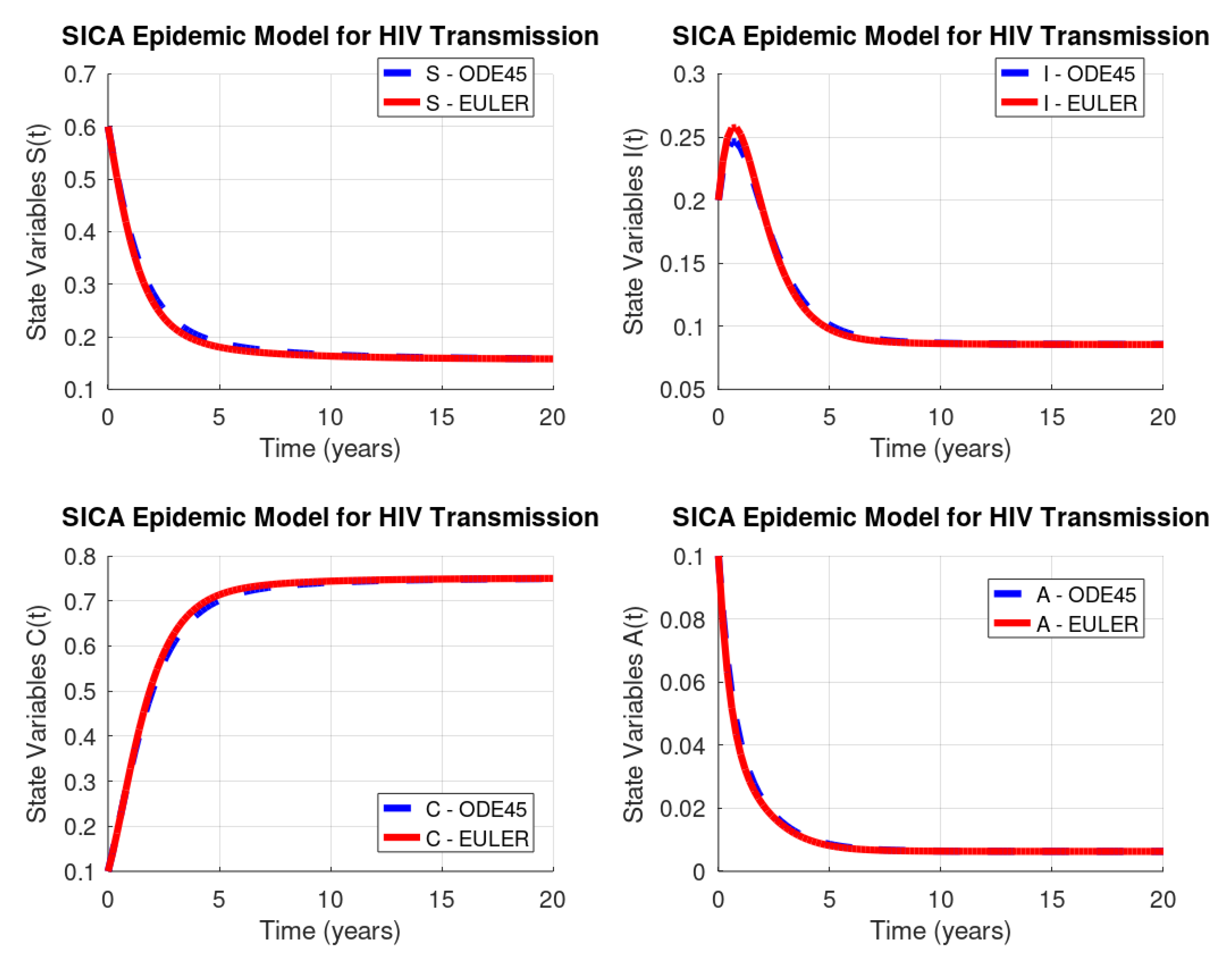
Figure 1 shows the solution of the system of ordinary differential equations (Equation (2)) with the initial conditions (Equation (3)), computed by the ode45 GNU Octave function (dashed line) versus the implemented Euler’s method (solid line). As depicted, Euler’s method, although being the simplest method, gives a very good approximation to the behaviour of each of the four system variables. Both implementations use the same discretization knots in the interval with a step size given by .
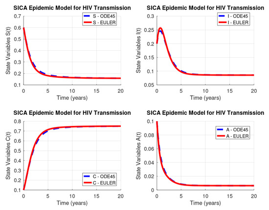
Figure 1.
HIV/AIDS system (Equation (2)) behaviour: GNU Octave versus Euler’s method.
Euler’s method has a global error (total accumulated error) of , and therefore, the error bound depends linearly on the step size h, which implies that the error is expected to grow in no worse than a linear manner. Consequently, diminishing the step size should give correspondingly greater accuracy to the approximations. Table 2 lists the norm of the difference vector, where each component of this vector is the absolute difference between the results obtained by the ode45 GNU Octave function and our implementation of Euler’s method, calculated by the vector norms 1, 2, and ∞.

Table 2.
Norms 1, 2, and ∞ of the difference vector between ode45 GNU Octave and Euler’s results.
3.3. Runge–Kutta of Order Two
Given a well-posed initial-value problem, the Runge–Kutta method of order two constructs a sequence of approximation points to the exact solution of the ordinary differential equation by , , , and , for each , where , , and . Our GNU Octave implementation of the Runge–Kutta method of order two applies the above formulation to approximate each of the four variables of the system in Equation (2). We implement the odeRungeKutta_order2 function through the following GNU Octave instructions:
- function dy = odeRungeKutta_order2(T)
- % Parameters of the modelmi = 1.0 / 69.54; b = 2.1 * mi; beta = 1.6;etaC = 0.015; etaA = 1.3; fi = 1.0; ro = 0.1;alfa = 0.33; omega = 0.09; d = 1.0;
- % Parameters of the Runge-Kutta (2nd order) methodtest = -1; deltaError = 0.001; M = 100;t = linspace(0,T,M+1); h = T / M; h2 = h / 2;S = zeros(1,M+1); I = zeros(1,M+1);C = zeros(1,M+1); A = zeros(1,M+1);
- % Initial conditions of the modelS(1) = 0.6; I(1) = 0.2; C(1) = 0.1; A(1) = 0.1;
- % Iterations of the methodwhile(test < 0)
- oldS = S; oldI = I; oldC = C; oldA = A;for i = 1:M
- % Differential equations of the model% First Runge-Kutta parameteraux1 = beta * (I(i) + etaC * C(i) + etaA * A(i)) * S(i);aux2 = d * A(i);auxS1 = b * (1 - S(i)) - aux1 + aux2 * S(i);auxI1 = aux1 - (ro + fi + b - aux2) * I(i) + alfa * A(i) + omega * C(i);auxC1 = fi * I(i) - (omega + b - aux2) * C(i);auxA1 = ro * I(i) - (alfa + b + d - aux2) * A(i);% Second Runge-Kutta parameterauxS = S(i) + h * auxS1; auxI = I(i) + h * auxI1;auxC = C(i) + h * auxC1; auxA = A(i) + h * auxA1;aux1 = beta * (auxI + etaC * auxC + etaA * auxA) * auxS;aux2 = d * auxA;auxS2 = b * (1 - auxS) - aux1 + aux2 * auxS;auxI2 = aux1 - (ro + fi + b - aux2) * auxI + alfa * auxA + omega * auxC;auxC2 = fi * auxI - (omega + b - aux2) * auxC;auxA2 = ro * auxI - (alfa + b + d - aux2) * auxA;% Runge-Kutta new approximationS(i+1) = S(i) + h2 * (auxS1 + auxS2);I(i+1) = I(i) + h2 * (auxI1 + auxI2);C(i+1) = C(i) + h2 * (auxC1 + auxC2);A(i+1) = A(i) + h2 * (auxA1 + auxA2);
- end% Absolute error for convergencetemp1 = deltaError * sum(abs(S)) - sum(abs(oldS - S));temp2 = deltaError * sum(abs(I)) - sum(abs(oldI - I));temp3 = deltaError * sum(abs(C)) - sum(abs(oldC - C));temp4 = deltaError * sum(abs(A)) - sum(abs(oldA - A));test = min(temp1,min(temp2,min(temp3,temp4)));
- enddy(1,:) = t; dy(2,:) = S; dy(3,:) = I;dy(4,:) = C; dy(5,:) = A;
Figure 2 shows the solution of the system of Equation (2) with the initial value conditions in Equation (3) computed by the ode45 GNU Octave function (dashed line) versus our implementation of the Runge–Kutta method of order two (solid line). As we can see, Runge–Kutta’s method produces a better approximation than Euler’s method, since both curves in each plot of Figure 2 are indistinguishable.
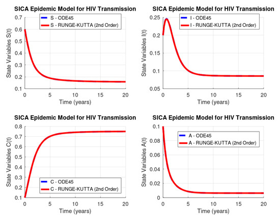
Figure 2.
HIV/AIDS system (Equation (2)): GNU Octave versus Runge–Kutta’s method of order two.
Runge–Kutta’s method of order two (RK2) has a global truncation error of order , and as it is known, this truncation error at a specified step measures the amount by which the exact solution to the differential equation fails to satisfy the difference equation being used for the approximation at that step. This might seems like an unlikely way to compare the error of various methods, since we really want to know how well the approximations generated by the methods satisfy the differential equation, not the other way around. However, we do not know the exact solution, so we cannot generally determine this, and the truncation error will serve quite well to determine not only the error of a method but also the actual approximation error. Table 3 lists the norm of the difference vector between the results from ode45 routine and Runge–Kutta’s method of order two results.

Table 3.
Norms 1, 2, and ∞ of the difference vector between ode45 GNU Octave and RK2 results.
3.4. Runge–Kutta of Order Four
The Runge–Kutta method of order four (RK4) constructs a sequence of approximation points to the exact solution of an ordinary differential equation by , , , , , and , for each , where , , and . Our GNU Octave implementation of the Runge–Kutta method of order four applies the above formulation to approximate the solution of the system in Equation (2) with the initial conditions of Equation (3) through the following instructions:
- function dy = odeRungeKutta_order4(T)
- % Parameters of the modelmi = 1.0 / 69.54; b = 2.1 * mi; beta = 1.6;etaC = 0.015; etaA = 1.3; fi = 1.0; ro = 0.1;alfa = 0.33; omega = 0.09; d = 1.0;
- % Parameters of the Runge-Kutta (4th order) methodtest = -1; deltaError = 0.001; M = 100;t = linspace(0,T,M+1);h = T / M; h2 = h / 2; h6 = h / 6;S = zeros(1,M+1); I = zeros(1,M+1);C = zeros(1,M+1); A = zeros(1,M+1);
- % Initial conditions of the modelS(1) = 0.6; I(1) = 0.2; C(1) = 0.1; A(1) = 0.1;% Iterations of the methodwhile(test < 0)
- oldS = S; oldI = I; oldC = C; oldA = A;for i = 1:M
- % Differential equations of the model% First Runge-Kutta parameteraux1 = beta * (I(i) + etaC * C(i) + etaA * A(i)) * S(i);aux2 = d * A(i);auxS1 = b * (1 - S(i)) - aux1 + aux2 * S(i);auxI1 = aux1 - (ro + fi + b - aux2) * I(i) + alfa * A(i) + omega * C(i);auxC1 = fi * I(i) - (omega + b - aux2) * C(i);auxA1 = ro * I(i) - (alfa + b + d - aux2) * A(i);
- % Second Runge-Kutta parameterauxS = S(i) + h2 * auxS1; auxI = I(i) + h2 * auxI1;auxC = C(i) + h2 * auxC1; auxA = A(i) + h2 * auxA1;aux1 = beta * (auxI + etaC * auxC + etaA * auxA) * auxS;aux2 = d * auxA;
- auxS2 = b * (1 - auxS) - aux1 + aux2 * auxS;auxI2 = aux1 - (ro + fi + b - aux2) * auxI + alfa * auxA + omega * auxC;auxC2 = fi * auxI - (omega + b - aux2) * auxC;auxA2 = ro * auxI - (alfa + b + d - aux2) * auxA;
- % Fird Runge-Kutta parameterauxS = S(i) + h2 * auxS2; auxI = I(i) + h2 * auxI2;auxC = C(i) + h2 * auxC2; auxA = A(i) + h2 * auxA2;aux1 = beta * (auxI + etaC * auxC + etaA * auxA) * auxS;aux2 = d * auxA;
- auxS3 = b * (1 - auxS) - aux1 + aux2 * auxS;auxI3 = aux1 - (ro + fi + b - aux2) * auxI + alfa * auxA + omega * auxC;auxC3 = fi * auxI - (omega + b - aux2) * auxC;auxA3 = ro * auxI - (alfa + b + d - aux2) * auxA;
- % Fourth Runge-Kutta parameterauxS = S(i) + h * auxS3; auxI = I(i) + h * auxI3;auxC = C(i) + h * auxC3; auxA = A(i) + h * auxA3;aux1 = beta * (auxI + etaC * auxC + etaA * auxA) * auxS;aux2 = d * auxA;
- auxS4 = b * (1 - auxS) - aux1 + aux2 * auxS;auxI4 = aux1 - (ro + fi + b - aux2) * auxI + alfa * auxA + omega * auxC;auxC4 = fi * auxI - (omega + b - aux2) * auxC;auxA4 = ro * auxI - (alfa + b + d - aux2) * auxA;
- % Runge-Kutta new approximationS(i+1) = S(i) + h6 * (auxS1 + 2 * (auxS2 + auxS3) + auxS4);I(i+1) = I(i) + h6 * (auxI1 + 2 * (auxI2 + auxI3) + auxI4);C(i+1) = C(i) + h6 * (auxC1 + 2 * (auxC2 + auxC3) + auxC4);A(i+1) = A(i) + h6 * (auxA1 + 2 * (auxA2 + auxA3) + auxA4);
- end
- % Absolute error for convergencetemp1 = deltaError * sum(abs(S)) - sum(abs(oldS - S));temp2 = deltaError * sum(abs(I)) - sum(abs(oldI - I));temp3 = deltaError * sum(abs(C)) - sum(abs(oldC - C));temp4 = deltaError * sum(abs(A)) - sum(abs(oldA - A));test = min(temp1,min(temp2,min(temp3,temp4)));
- enddy(1,:) = t; dy(2,:) = S; dy(3,:) = I;dy(4,:) = C; dy(5,:) = A;
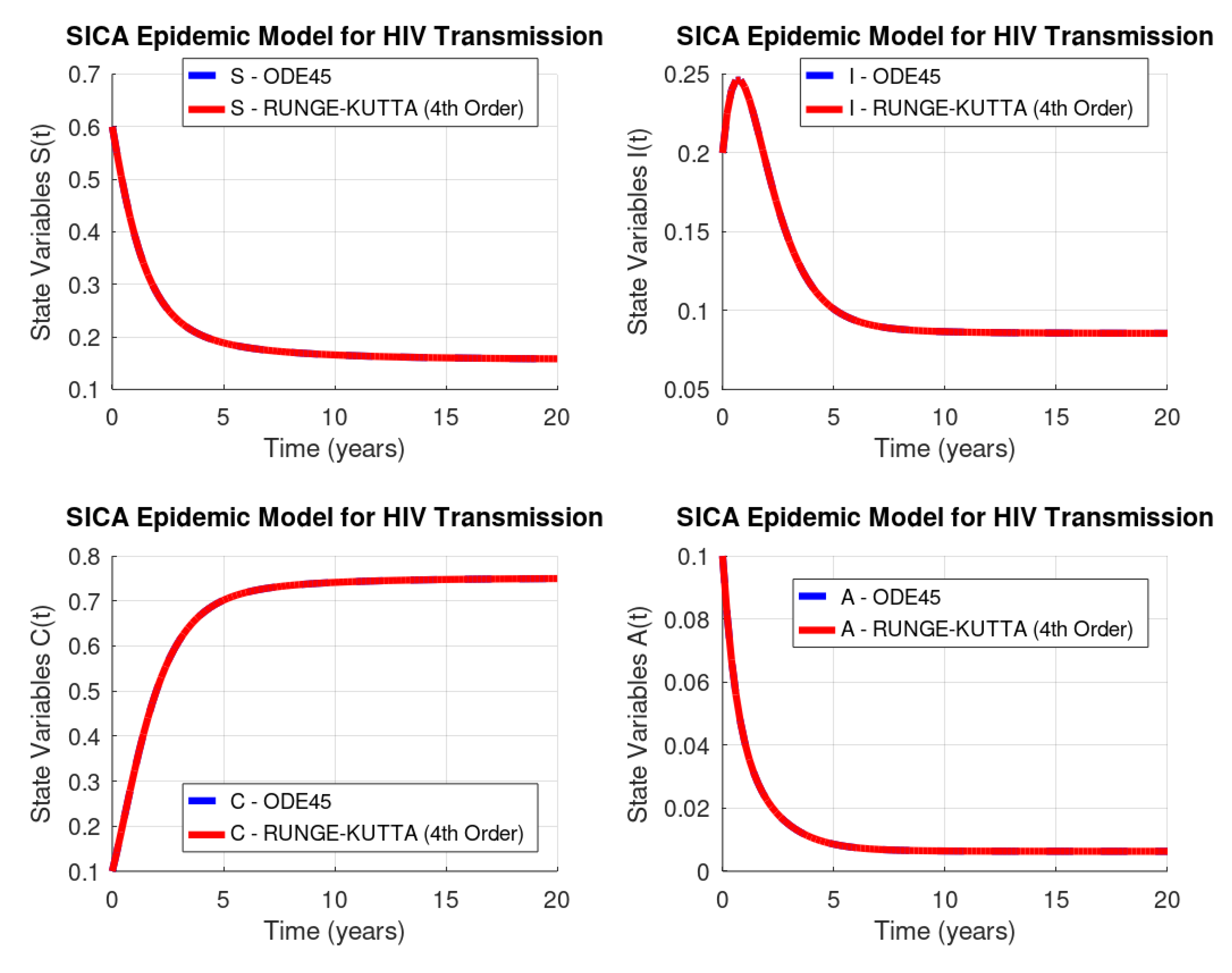
Figure 3 shows the solution of the initial value problem in Equations (2) and (3) computed by the ode45 GNU Octave function (dashed line) versus our implementation of the Runge–Kutta method of order four (solid line). The results of the Runge–Kutta method of order four are extremely good. Moreover, this method requires four evaluations per step and its global truncation error is .
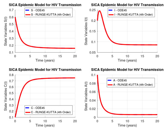
Figure 3.
HIV/AIDS system (Equation (2)): GNU Octave versus Runge–Kutta’s method of order four.
Table 4 lists the norm of the difference vector between results obtained by the Octave routine ode45 and the 4th order Runge–Kutta method.

Table 4.
Norms 1, 2, and ∞ of the difference vector between ode45 GNU Octave and RK4 results.
4. Optimal Control of HIV Transmission
In this section, we propose an optimal control problem that will be solved numerically in Octave/MATLAB in Section 4.2. We introduce a control function in the model of Equation (2), which represents the effort on HIV prevention measures, such as condom use (used consistently and correctly during every sex act) or oral pre-exposure prophylasis (PrEP). The control system is given by
where the control is bounded between 0 and , with . When the control vanishes, no extra preventive measure for HIV transmission is being used by susceptible individuals. We assume that is never equal to 1, since it makes the model more realistic from a medical point of view.
The goal is to find the optimal value of the control u along time, such that the associated state trajectories , , , and are solutions of the system in Equation (4) in the time interval with the following initial given conditions:
and maximizes the objective functional given by
which considers the fraction of susceptible individuals (s) and HIV-infected individuals without AIDS symptoms (i) and the cost associated with the support of HIV transmission measures (u).
The control system in Equation (4) of ordinary differential equations in is considered with the set of admissible control functions given by
We consider the optimal control problem of determining associated to an admissible control on the time interval , satisfying Equation (4) and the initial conditions of Equation (5) and maximizing the cost functional of Equation (6):
Note that we are considering a -cost function: the integrand of the cost functional J is concave with respect to the control u. Moreover, the control system of Equation (4) is Lipschitz with respect to the state variables . These properties ensure the existence of an optimal control of the optimal control problem in Equations (4)–(8) (see, e.g., Reference [14]).
To solve optimal control problems, two approaches are possible: direct and indirect. Direct methods consist in the discretization of the optimal control problem, reducing it to a nonlinear programming problem [15,16]. For such an approach, one only needs to use the Octave/MATLAB fmincon routine. Indirect methods are more sound because they are based on Pontryagin’s Maximum Principle but less widespread since they are not immediately available in Octave/MATLAB. Here, we show how one can use Octave/MATLAB to solve optimal control problems through Pontryagin’s Maximum Principle, reducing the optimal control problem to the solution of a boundary value problem.
4.1. Pontryagin’s Maximum Principle
According to celebrated Pontryagin’s Maximum Principle (see, e.g., Reference [3]), if is optimal for Equations (4)–(8) with fixed final time T, then there exists a nontrivial absolutely continuous mapping , , called the adjoint vector, such that
where
is called the Hamiltonian and the maximality condition
holds almost everywhere on . Moreover, the transversality conditions
hold. Applying the Pontryagin maximum principle to the optimal control problem in Equations (4)–(8), the following theorem follows.
Theorem 1.
Remark 1.
We implement Theorem 1 numerically in Octave/MATLAB in Section 4.2, and the optimal solution associated to the optimal control is computed for given parameter values and initial conditions.
4.2. Numerical Solution of the HIV Optimal Control Problem
The extremal given by Theorem 1 is now computed numerically by implementing a forward-backward fourth-order Runge–Kutta method (see, e.g., Reference [19]). This iterative method consists in solving the system in Equation (4) with a guess for the controls over the time interval using a forward fourth-order Runge–Kutta scheme and the transversality conditions , . Then, the adjoint system in Equation (10) is solved by a backward fourth-order Runge–Kutta scheme using the current iteration solution of Equation (4). The controls are updated by using a convex combination of the previous controls and the values from Equation (9). The iteration is stopped if the values of unknowns at the previous iteration are very close to the ones at the present iteration. Our odeRungeKutta_order4_WithControl function is implemented by the following GNU Octave instructions:
- function dy = odeRungeKutta_order4_WithControl(T)
- % Parameters of the modelmi = 1.0 / 69.54; b = 2.1 * mi; beta = 1.6;etaC = 0.015; etaA = 1.3; fi = 1.0; ro = 0.1;alfa = 0.33; omega = 0.09; d = 1.0;
- % Parameters of the Runge-Kutta (4th order) methodtest = -1; deltaError = 0.001; M = 1000;t = linspace(0,T,M+1);h = T / M; h2 = h / 2; h6 = h / 6;S = zeros(1,M+1); I = zeros(1,M+1);C = zeros(1,M+1); A = zeros(1,M+1);
- % Initial conditions of the modelS(1) = 0.6; I(1) = 0.2; C(1) = 0.1; A(1) = 0.1;
- %Vectors for system restrictions and controlLambda1 = zeros(1,M+1); Lambda2 = zeros(1,M+1);Lambda3 = zeros(1,M+1); Lambda4 = zeros(1,M+1);U = zeros(1,M+1);% Iterations of the methodwhile(test < 0)
- oldS = S; oldI = I; oldC = C; oldA = A;oldLambda1 = Lambda1; oldLambda2 = Lambda2;oldLambda3 = Lambda3; oldLambda4 = Lambda4;oldU = U;
- %Forward Runge-Kutta iterationsfor i = 1:M
- % Differential equations of the model% First Runge-Kutta parameteraux1 = (1 - U(i)) * beta * (I(i) + etaC * C(i) + etaA * A(i)) * S(i);aux2 = d * A(i);
- auxS1 = b * (1 - S(i)) - aux1 + aux2 * S(i);auxI1 = aux1 - (ro + fi + b - aux2) * I(i) + alfa * A(i) + omega * C(i);auxC1 = fi * I(i) - (omega + b - aux2) * C(i);auxA1 = ro * I(i) - (alfa + b + d - aux2) * A(i);
- % Second Runge-Kutta parameterauxU = 0.5 * (U(i) + U(i+1));auxS = S(i) + h2 * auxS1; auxI = I(i) + h2 * auxI1;auxC = C(i) + h2 * auxC1; auxA = A(i) + h2 * auxA1;aux1 = (1 - auxU) * beta * (auxI + etaC * auxC + etaA * auxA) * auxS;aux2 = d * auxA;auxS2 = b * (1 - auxS) - aux1 + aux2 * auxS;auxI2 = aux1 - (ro + fi + b - aux2) * auxI + alfa * auxA + omega * auxC;auxC2 = fi * auxI - (omega + b - aux2) * auxC;auxA2 = ro * auxI - (alfa + b + d - aux2) * auxA;
- % Third Runge-Kutta parameterauxS = S(i) + h2 * auxS2; auxI = I(i) + h2 * auxI2;auxC = C(i) + h2 * auxC2; auxA = A(i) + h2 * auxA2;aux1 = (1 - auxU) * beta * (auxI + etaC * auxC + etaA * auxA) * auxS;aux2 = d * auxA;
- auxS3 = b * (1 - auxS) - aux1 + aux2 * auxS;auxI3 = aux1 - (ro + fi + b - aux2) * auxI + alfa * auxA + omega * auxC;auxC3 = fi * auxI - (omega + b - aux2) * auxC;auxA3 = ro * auxI - (alfa + b + d - aux2) * auxA;
- % Fourth Runge-Kutta parameterauxS = S(i) + h * auxS3; auxI = I(i) + h * auxI3;auxC = C(i) + h * auxC3; auxA = A(i) + h * auxA3;aux1 = (1 - U(i+1)) * beta * (auxI + etaC * auxC + etaA * auxA) * auxS;aux2 = d * auxA;
- auxS4 = b * (1 - auxS) - aux1 + aux2 * auxS;auxI4 = aux1 - (ro + fi + b - aux2) * auxI + alfa * auxA + omega * auxC;auxC4 = fi * auxI - (omega + b - aux2) * auxC;auxA4 = ro * auxI - (alfa + b + d - aux2) * auxA;
- % Runge-Kutta new approximationS(i+1) = S(i) + h6 * (auxS1 + 2 * (auxS2 + auxS3) + auxS4);I(i+1) = I(i) + h6 * (auxI1 + 2 * (auxI2 + auxI3) + auxI4);C(i+1) = C(i) + h6 * (auxC1 + 2 * (auxC2 + auxC3) + auxC4);A(i+1) = A(i) + h6 * (auxA1 + 2 * (auxA2 + auxA3) + auxA4);
- end
- %Backward Runge-Kutta iterationsfor i = 1:M
- j = M + 2 - i;
- % Differential equations of the model% First Runge-Kutta parameterauxU = 1 - U(j);aux1 = auxU * beta * (I(j) + etaC * C(j) + etaA * A(j));aux2 = d * A(j);
- auxLambda11 = -1 + Lambda1(j) * (b + aux1 - aux2) - Lambda2(j) * aux1;aux1 = auxU * beta * S(j);auxLambda21 = 1 + Lambda1(j) * aux1 - Lambda2(j) * (aux1 - (ro + fi + b) + ...+ aux2) - Lambda3(j) * fi - Lambda4(j) * ro;aux1 = auxU * beta * etaC * S(j);auxLambda31 = Lambda1(j) * aux1 - Lambda2(j) * (aux1 + ...+ omega) + Lambda3(j) * (omega + b - aux2);aux1 = auxU * beta * etaA * S(j);auxLambda41 = Lambda1(j) * (aux1 + d * S(j)) ...- Lambda2(j) * (aux1 + alfa + ...+ d * I(j)) - Lambda3(j) * d * C(j) + ...+ Lambda4(j) * (alfa + b + d - 2 * aux2);
- % Second Runge-Kutta parameterauxU = 1 - 0.5 * (U(j) + U(j-1));auxS = 0.5 * (S(j) + S(j-1));auxI = 0.5 * (I(j) + I(j-1));auxC = 0.5 * (C(j) + C(j-1));auxA = 0.5 * (A(j) + A(j-1));
- aux1 = auxU * beta * (auxI + etaC * auxC + etaA * auxA);aux2 = d * auxA;auxLambda1 = Lambda1(j) - h2 * auxLambda11;auxLambda2 = Lambda2(j) - h2 * auxLambda21;auxLambda3 = Lambda3(j) - h2 * auxLambda31;auxLambda4 = Lambda4(j) - h2 * auxLambda41;
- auxLambda12 = -1 + auxLambda1 * (b + aux1 - aux2) - auxLambda2 * aux1;aux1 = auxU * beta * auxS;auxLambda22 = 1 + auxLambda1 * aux1 - auxLambda2 * (aux1 - (ro + fi + b) + ...+ aux2) - auxLambda3 * fi - auxLambda4 * ro;aux1 = auxU * beta * etaC * auxS;auxLambda32 = auxLambda1 * aux1 - auxLambda2 * (aux1 + ...+ omega) + auxLambda3 * (omega + b - aux2);aux1 = auxU * beta * etaA * auxS;auxLambda42 = auxLambda1 * (aux1 + d * auxS) ...- auxLambda2 * (aux1 + alfa + ...+ d * auxI) - auxLambda3 * d * auxC + ...+ auxLambda4 * (alfa + b + d - 2 * aux2);
- % Third Runge-Kutta parameteraux1 = auxU * beta * (auxI + etaC * auxC + etaA * auxA);auxLambda1 = Lambda1(j) - h2 * auxLambda12;auxLambda2 = Lambda2(j) - h2 * auxLambda22;auxLambda3 = Lambda3(j) - h2 * auxLambda32;auxLambda4 = Lambda4(j) - h2 * auxLambda42;
- auxLambda13 = -1 + auxLambda1 * (b + aux1 - aux2) - auxLambda2 * aux1;aux1 = auxU * beta * auxS;auxLambda23 = 1 + auxLambda1 * aux1 ...- auxLambda2 * (aux1 - (ro + fi + b) + ...+ aux2) - auxLambda3 * fi - auxLambda4 * ro;aux1 = auxU * beta * etaC * auxS;auxLambda33 = auxLambda1 * aux1 - auxLambda2 * (aux1 + ...+ omega) + auxLambda3 * (omega + b - aux2);aux1 = auxU * beta * etaA * auxS;auxLambda43 = auxLambda1 * (aux1 + d * auxS) ...- auxLambda2 * (aux1 + alfa + d * auxI) - auxLambda3 * d * auxC + ...+ auxLambda4 * (alfa + b + d - 2 * aux2);% Fourth Runge-Kutta parameterauxU = 1 - U(j-1); auxS = S(j-1);auxI = I(j-1); auxC = C(j-1); auxA = A(j-1);
- aux1 = auxU * beta * (auxI + etaC * auxC + etaA * auxA);aux2 = d * auxA;auxLambda1 = Lambda1(j) - h * auxLambda13;auxLambda2 = Lambda2(j) - h * auxLambda23;auxLambda3 = Lambda3(j) - h * auxLambda33;auxLambda4 = Lambda4(j) - h * auxLambda43;
- auxLambda14 = -1 + auxLambda1 * (b + aux1 - aux2) ...- auxLambda2 * aux1;aux1 = auxU * beta * auxS;auxLambda24 = 1 + auxLambda1 * aux1 ...- auxLambda2 * (aux1 - (ro + fi + b) + ...+ aux2) - auxLambda3 * fi - auxLambda4 * ro;aux1 = auxU * beta * etaC * auxS;auxLambda34 = auxLambda1 * aux1 - auxLambda2 * (aux1 + ...+ omega) + auxLambda3 * (omega + b - aux2);aux1 = auxU * beta * etaA * auxS;auxLambda44 = auxLambda1 * (aux1 + d * auxS) ...- auxLambda2 * (aux1 + alfa + ...+ d * auxI) - auxLambda3 * d * auxC + ...+ auxLambda4 * (alfa + b + d - 2 * aux2);
- % Runge-Kutta new approximationLambda1(j-1) = Lambda1(j) - h6 * (auxLambda11 + ...+ 2 * (auxLambda12 + auxLambda13) + auxLambda14);Lambda2(j-1) = Lambda2(j) - h6 * (auxLambda21 + ...+ 2 * (auxLambda22 + auxLambda23) + auxLambda24);Lambda3(j-1) = Lambda3(j) - h6 * (auxLambda31 + ...+ 2 * (auxLambda32 + auxLambda33) + auxLambda34);Lambda4(j-1) = Lambda4(j) - h6 * (auxLambda41 + ...+ 2 * (auxLambda42 + auxLambda43) + auxLambda44);
- end
- % New vector controlfor i = 1:M+1
- vAux(i) = 0.5 * beta * (I(i) + etaC * C(i) + ...+ etaA * A(i)) * S(i) * (Lambda1(i) - Lambda2(i));auxU = min([max([0.0 vAux(i)]) 0.5]);U(i) = 0.5 * (auxU + oldU(i));
- end
- % Absolute error for convergencetemp1 = deltaError * sum(abs(S)) - sum(abs(oldS - S));temp2 = deltaError * sum(abs(I)) - sum(abs(oldI - I));temp3 = deltaError * sum(abs(C)) - sum(abs(oldC - C));temp4 = deltaError * sum(abs(A)) - sum(abs(oldA - A));temp5 = deltaError * sum(abs(U)) - sum(abs(oldU - U));temp6 = deltaError * sum(abs(Lambda1)) - sum(abs(oldLambda1 - Lambda1));temp7 = deltaError * sum(abs(Lambda2)) - sum(abs(oldLambda2 - Lambda2));temp8 = deltaError * sum(abs(Lambda3)) - sum(abs(oldLambda3 - Lambda3));temp9 = deltaError * sum(abs(Lambda4)) - sum(abs(oldLambda4 - Lambda4));test = min(temp1,min(temp2,min(temp3,min(temp4, ...min(temp5,min(temp6,min(temp7,min(temp8,temp9))))))));
- end
- dy(1,:) = t; dy(2,:) = S; dy(3,:) = I;dy(4,:) = C; dy(5,:) = A; dy(6,:) = U;disp("Value of LAMBDA at FINAL TIME");disp([Lambda1(M+1) Lambda2(M+1) Lambda3(M+1) Lambda4(M+1)]);
For the numerical simulations, we consider , representing a lack of resources or misuse of the preventive HIV measures , that is, the set of admissible controls is given by
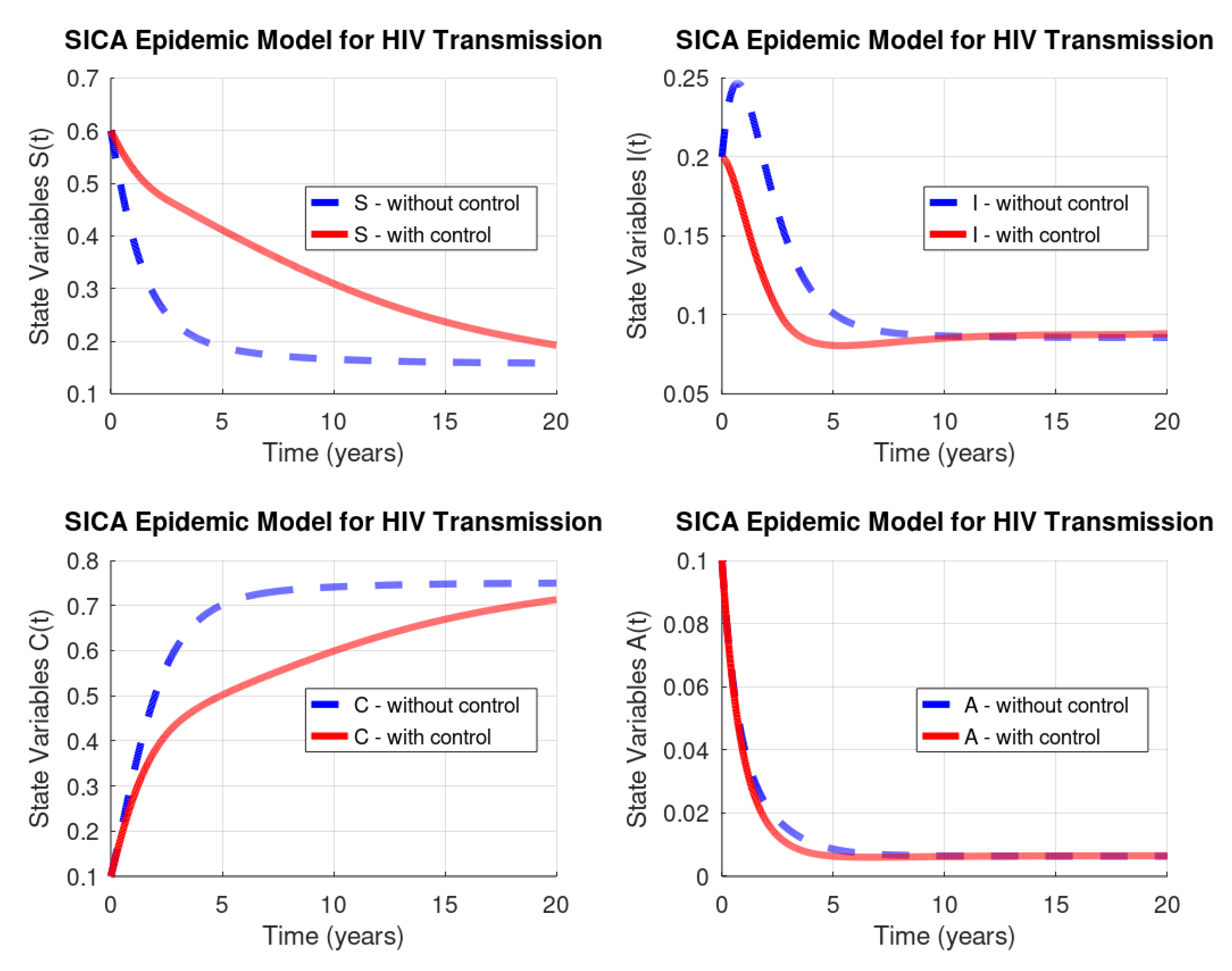
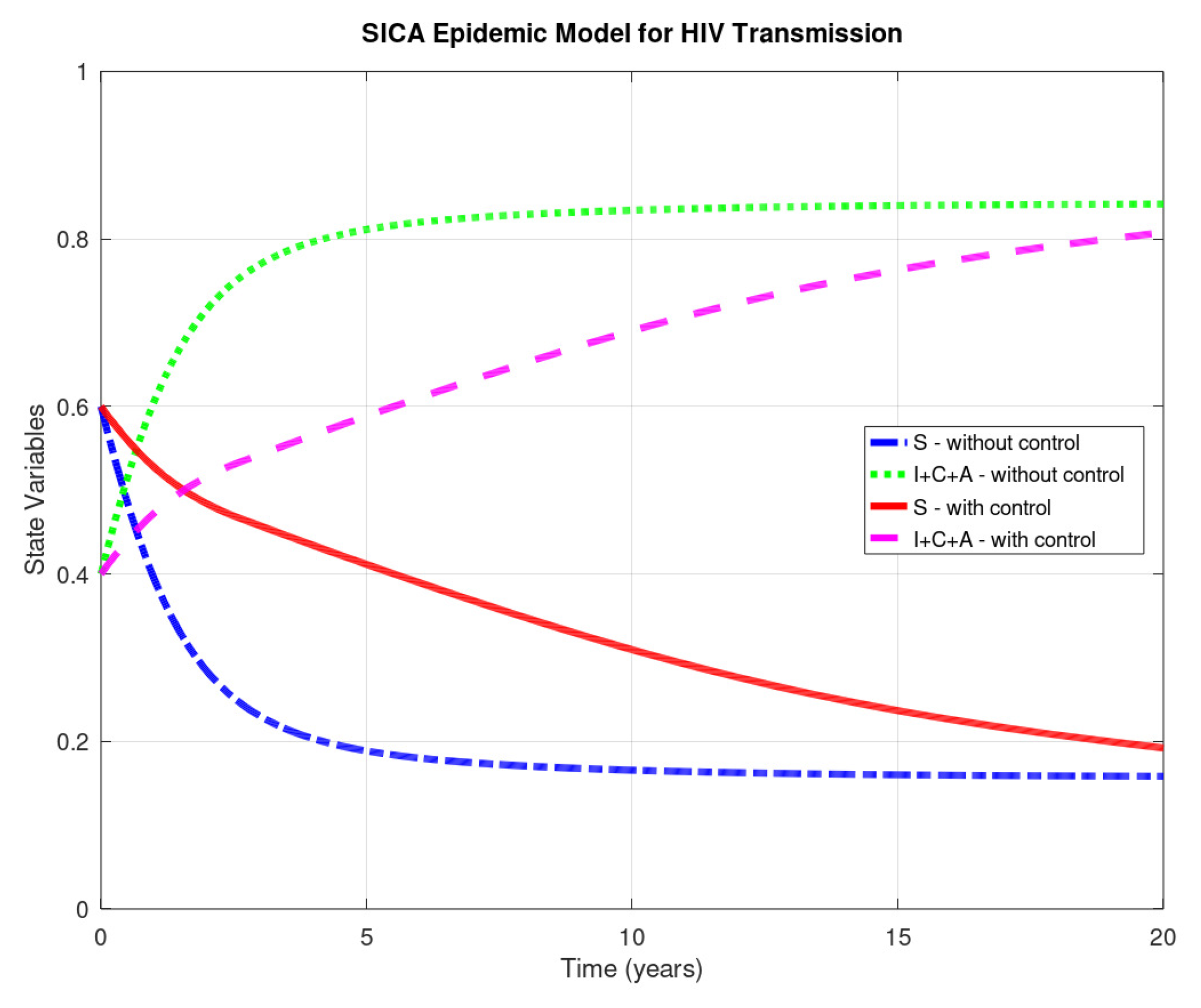
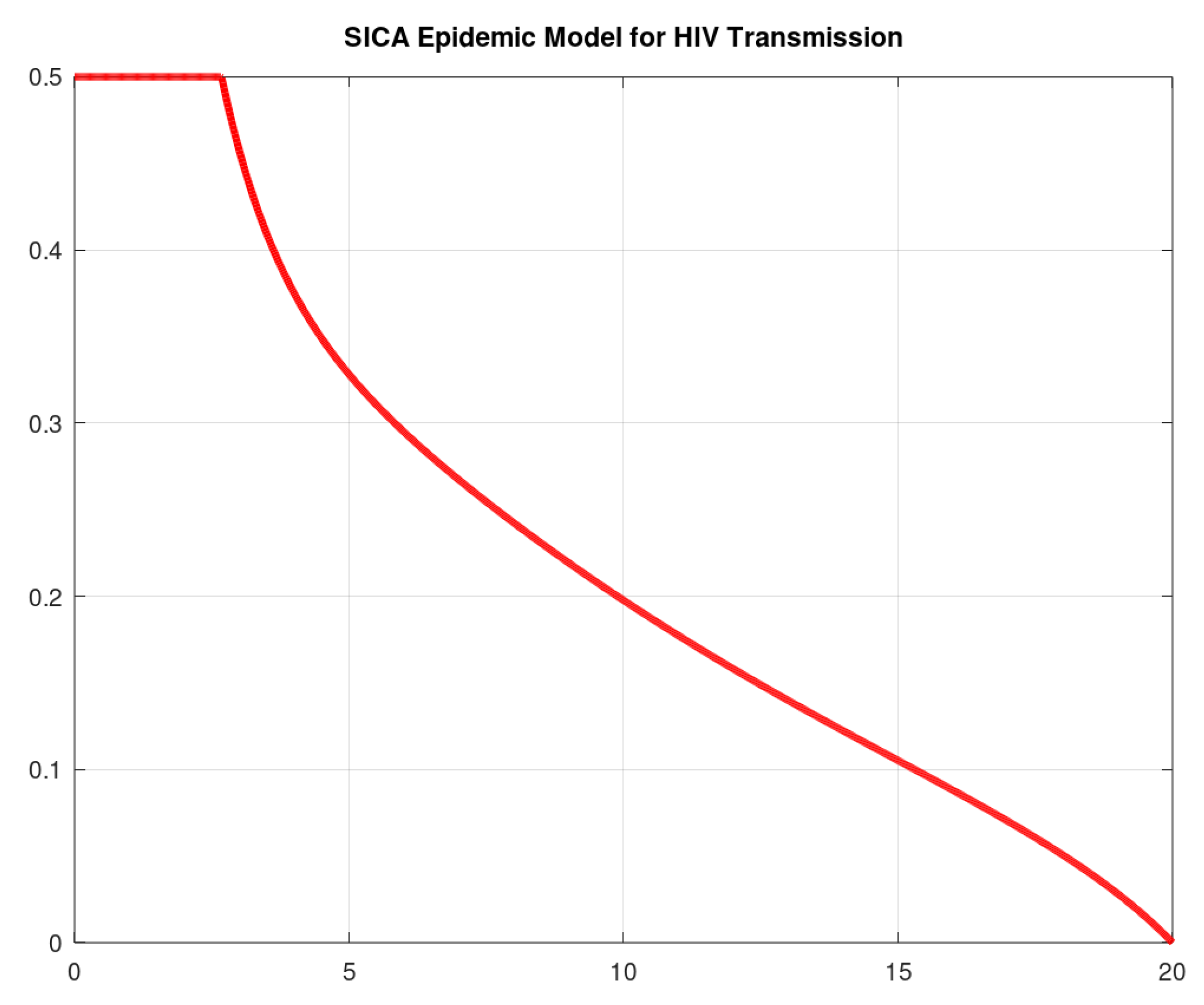
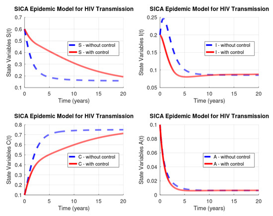
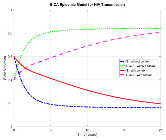
with (years). Figure 4 and Figure 5 show the numerical solution to the optimal control problem of Equations (4)–(8) with the initial conditions of Equation (3) and the admissible control set in Equation (11) computed by our odeRungeKutta_order4_WithControl function. Figure 6 depicts the extremal control behaviour of .
5. Conclusions
The paper provides a study on numerical methods to deal with modelling and optimal control of epidemic problems. Simple but effective Octave/MATLAB code is fully provided for a recent model proposed in Reference [10]. The given numerical procedures are robust with respect to the parameters: we have used the same values as the ones in Reference [10], but the code is valid for other values of the parameters and easily modified to other models. The results show the effectiveness of optimal control theory in medicine and the usefulness of a scientific computing system such as GNU Octave: using the control measure as predicted by Pontryagin’s maximum principle and numerically computed by our Octave code, one sees that the number of HIV/AIDS-infected and -chronic individuals diminish and, as a consequence, the number of susceptible (not ill) individuals increase. We trust our paper will be very useful to a practitioner from the disease control area. Indeed, this work has been motivated by many emails we received and continue to receive, asking us to provide the software code associated to our research papers on applications of optimal control theory in epidemiology, e.g., References [20,21].
Author Contributions
Each author equally contributed to this paper, read and approved the final manuscript. All authors have read and agreed to the published version of the manuscript.
Funding
This research was partially supported by the Portuguese Foundation for Science and Technology (FCT) within projects UID/MAT/04106/2019 (CIDMA) and PTDC/EEI-AUT/2933/2014 (TOCCATTA) and was cofunded by FEDER funds through COMPETE2020—Programa Operacional Competitividade e Internacionalização (POCI) and by national funds (FCT). Silva is also supported by national funds (OE), through FCT, I.P., in the scope of the framework contract foreseen in numbers 4–6 of article 23 of the Decree-Law 57/2016 of August 29, changed by Law 57/2017 of July 19.
Acknowledgments
The authors are sincerely grateful to four anonymous reviewers for several useful comments, suggestions, and criticisms, which helped them to improve the paper.
Conflicts of Interest
The authors declare no conflict of interest.
References
- Brauer, F.; Castillo-Chavez, C. Mathematical Models in Population Biology and Epidemiology, 2nd ed.; Springer: New York, NY, USA, 2012. [Google Scholar] [CrossRef]
- Elazzouzi, A.; Lamrani Alaoui, A.; Tilioua, M.; Torres, D.F.M. Analysis of a SIRI epidemic model with distributed delay and relapse. Stat. Optim. Inf. Comput. 2019, 7, 545–557. [Google Scholar] [CrossRef]
- Pontryagin, L.S.; Boltyanskii, V.G.; Gamkrelidze, R.V.; Mishchenko, E.F. The Mathematical Theory of Optimal Processes; Translated from the Russian by K.N. Trirogoff; Neustadt, L.W., Ed.; John Wiley & Sons, Inc.: New York, NY, USA, 1962. [Google Scholar]
- Area, I.; Ndaïrou, F.; Nieto, J.J.; Silva, C.J.; Torres, D.F.M. Ebola model and optimal control with vaccination constraints. J. Ind. Manag. Optim. 2018, 14, 427–446. [Google Scholar] [CrossRef]
- Burlacu, R.; Cavache, A. On a class of optimal control problems in mathematical biology. IFAC Proc. Vol. 1999, 32, 3746–3759. [Google Scholar] [CrossRef]
- Deshpande, S. Optimal Input Signal Design for Data-Centric Identification and Control with Applications to Behavioral Health and Medicine; ProQuest LLC: Ann Arbor, MI, USA, 2014. [Google Scholar]
- Silva, C.J.; Torres, D.F.M.; Venturino, E. Optimal spraying in biological control of pests. Math. Model. Nat. Phenom. 2017, 12, 51–64. [Google Scholar] [CrossRef][Green Version]
- Rosa, S.; Torres, D.F.M. Optimal control and sensitivity analysis of a fractional order TB model. Stat. Optim. Inf. Comput. 2019, 7, 617–625. [Google Scholar] [CrossRef]
- Allali, K.; Harroudi, S.; Torres, D.F.M. Analysis and optimal control of an intracellular delayed HIV model with CTL immune response. Math. Comput. Sci. 2018, 12, 111–127. [Google Scholar] [CrossRef]
- Silva, C.J.; Torres, D.F.M. A SICA compartmental model in epidemiology with application to HIV/AIDS in Cape Verde. Ecol. Complex. 2017, 30, 70–75. [Google Scholar] [CrossRef]
- Silva, C.J.; Torres, D.F.M. Modeling and optimal control of HIV/AIDS prevention through PrEP. Discrete Contin. Dyn. Syst. Ser. S 2018, 11, 119–141. [Google Scholar] [CrossRef]
- An, G. The Crisis of Reproducibility, the Denominator Problem and the Scientific Role of Multi-scale Modeling. Bull. Math. Biol. 2018, 80, 3071–3080. [Google Scholar] [CrossRef] [PubMed]
- Eaton, J.W.; Bateman, D.; Hauberg, S.; Wehbring, R. GNU Octave Version 5.1.0 Manual: A hIgh-Level Interactive Language for Numerical Computations. Available online: https://enacit.epfl.ch/cours/matlab-octave/octave-documentation/octave/octave.pdf (accessed on 6 October 2019).
- Cesari, L. Optimization—Theory and Applications; Springer: New York, NY, USA, 1983. [Google Scholar] [CrossRef]
- Salati, A.B.; Shamsi, M.; Torres, D.F.M. Direct transcription methods based on fractional integral approximation formulas for solving nonlinear fractional optimal control problems. Commun. Nonlinear Sci. Numer. Simul. 2019, 67, 334–350. [Google Scholar] [CrossRef]
- Nemati, S.; Lima, P.M.; Torres, D.F.M. A numerical approach for solving fractional optimal control problems using modified hat functions. Commun. Nonlinear Sci. Numer. Simul. 2019, 78, 104849. [Google Scholar] [CrossRef]
- Jung, E.; Lenhart, S.; Feng, Z. Optimal control of treatments in a two-strain tuberculosis model. Discrete Contin. Dyn. Syst. Ser. B 2002, 2, 473–482. [Google Scholar] [CrossRef]
- Silva, C.J.; Torres, D.F.M. Optimal control for a tuberculosis model with reinfection and post-exposure interventions. Math. Biosci. 2013, 244, 154–164. [Google Scholar] [CrossRef] [PubMed]
- Lenhart, S.; Workman, J.T. Optimal Control Applied to Biological Models; Chapman & Hall/CRC: Boca Raton, FL, USA, 2007. [Google Scholar]
- Rachah, A.; Torres, D.F.M. Mathematical modelling, simulation, and optimal control of the 2014 Ebola outbreak in West Africa. Discrete Dyn. Nat. Soc. 2015. [Google Scholar] [CrossRef]
- Malinzi, J.; Ouifki, R.; Eladdadi, A.; Torres, D.F.M.; White, K.A.J. Enhancement of chemotherapy using oncolytic virotherapy: Mathematical and optimal control analysis. Math. Biosci. Eng. 2018, 15, 1435–1463. [Google Scholar] [CrossRef] [PubMed]
© 2019 by the authors. Licensee MDPI, Basel, Switzerland. This article is an open access article distributed under the terms and conditions of the Creative Commons Attribution (CC BY) license (http://creativecommons.org/licenses/by/4.0/).


