Article

Almost Exact Computation of Eigenvalues in Approximate Differential Problems

1
Instituto Superior de Engenharia do Porto, Rua Dr. António Bernardino de Almeida, 431, 4249-015 Porto, Portugal
2
Centro de Matemática da Universidade do Porto, Rua do Campo Alegre, 687, 4169-007 Porto, Portugal
3
Faculdade de Ciências da Universidade do Porto, Rua do Campo Alegre, s/n, 4169-007 Porto, Portugal
*
Author to whom correspondence should be addressed.
Math. Comput. Appl. 2019, 24(4), 96; https://doi.org/10.3390/mca24040096
Submission received: 29 September 2019 / Revised: 12 November 2019 / Accepted: 13 November 2019 / Published: 14 November 2019
(This article belongs to the Special Issue Numerical and Symbolic Computation: Developments and Applications)

Abstract

:
Differential eigenvalue problems arise in many fields of Mathematics and Physics, often arriving, as auxiliary problems, when solving partial differential equations. In this work, we present a method for eigenvalues computation following the Tau method philosophy and using Tau Toolbox tools. This Matlab toolbox was recently presented and here we explore its potential use and suitability for this problem. The first step is to translate the eigenvalue differential problem into an algebraic approximated eigenvalues problem. In a second step, making use of symbolic computations, we arrive at the exact polynomial expression of the determinant of the algebraic problem matrix, allowing us to get high accuracy approximations of differential eigenvalues.

1. Introduction

Finding eigenfunctions of differential problems can be a hard task, at least for some classical problems. Among others, we can find literature in Sturm–Liouville problems, in Mathieu problems or in Orr–Sommerfeld problems describing the difficulties involved in the resolution of those problems [1,2,3,4,5,6,7,8]. The first difficulty consists of finding accurate numerical approximations for the respective eigenvalues.
In this work, we present a procedure based on the Ortiz and Samara’s operational approach to the Tau method described in [9], where the differential problem is translated into an algebraic problem. This is achieved using the called operational matrices that represent the action of differential operators in a function. We have deduced explicit formulae for the elements of these matrices [10,11] obtained by performing operations on the bases of orthogonal polynomials and, for some families, we have exact formulae, which enables the construction of very accurate operational matrices. The Tau method has already been used for these kinds of problems [5,9,12,13]; however, our work on matrix calculation formulas adds efficiency and precision to the method.
Our main purpose is to use the Tau Toolbox, a Matlab numerical library that is being developed by our research group [14,15,16]. This library allows a stable implementation of the Tau method for the construction of accurate approximate solutions for integro-differential problems. In particular, the construction of the operational matrices is done automatically. These facts led us to think that the Tau Toolbox seems to be useful for these kinds of problems.
Finally, operating with symbolic variables, we define the determinant of those matrices as polynomials and use its roots as eigenvalues’ approximations.
We present some examples showing that, using this technique in the Tau Toolbox, we are able to obtain results comparable with those reported in the literature and sometimes even better.

2. The Tau Method

Let D : E F be an order ν differential operator, where E and F are some function spaces, and let g i : E R , i = 1 , , ν be ν functionals representing boundary conditions, so that
D y = f , f F , g i ( y ) = ϕ i , i = 1 , , ν
is a well posed differential problem.

2.1. The Tau Method Principle

A particular implementation of the Tau method depends on the choice of an orthogonal basis for F . A sequence of orthogonal polynomials { P n ( x ) } n = 0 with respect to the weight function w ( x ) on a given interval of orthogonality [ a , b ] satisfies
P i , P j = a b w ( x ) P i ( x ) P j ( x ) d x = w i δ i j ,
where w i = P i , P i and δ i j is the Kronecker delta [17].
Let P be the space of algebraic polynomials of any degree and let us suppose that P is dense in F ; then, the solution y of (1) has a series representation y j 1 a j P j 1 . A polynomial approximation of degree n 1 N is achieved by
y n = j = 1 n a n , j P j 1 = P n a n ,
where P n = [ P 0 , P 1 , , P n 1 ] and a n = [ a n , 1 , , a n , n ] T .
In the Tau method sense, y n is a polynomial satisfying the boundary conditions in (1) and solving the differential equation with a residual τ n = D y n f of maximal order. Thus, the differential problem is reduced to an algebraic one of finding the n coefficients a n , j , j = 1 , , n in (2) such that
g i ( y n ) = ϕ i , i = 1 , , ν , P i 1 , D y n f = 0 , i = 1 , , n ν ,
and so the residual τ n = O ( P n ν ) .

2.2. Operational Formulation

For a given n N , n > ν , we define the matrix
T n = B ν × n D ( n ν ) × n = ( t i , j ) i , j = 1 n : t i , j = g i ( P j 1 ) , i = 1 , , ν P i ν 1 , D P j 1 w i ν 1 , i = ν + 1 , , n
and the vector
b n = g ν f n ν = ( b i ) i = 1 n : b i = ϕ i , i = 1 , , ν P i ν 1 , f w i ν 1 , i = ν + 1 , , n .
If, in problem (1), the differential operator D is linear and the g j are ν linear functionals, then problem (3) can be put in matrix form as
T n a n = b n .
The matrix T n , called the Tau matrix, can be evaluated from operational matrices, that is, matrices translating into coefficients vectors the action of a differential operator D in a function y.
Proposition 1.
Let P = [ P 0 , P 1 , ] be an orthogonal polynomial basis, y = P a and M , N infinite matrices such that
x P = P M and d d x P = P N .
Then, for each k N 0 ,
x k y = P M k a and d k d x k y = P N k a .
Proof. 
For k = 1 , the result is true by hypothesis. Now, supposing that (5) is true for a k N , then
x k + 1 y = x ( x k y ) = ( x P ) M k a = P M k + 1 a
and
d k + 1 d x k + 1 y = d d x ( d k d x k y ) = ( d d x P ) N k a = P N k + 1 a ,
ending the proof by induction. □
The following result generalizes the algebraic representation from the previous proposition to differential operators.
Corollary 1.
Let D : P n P n + h be a linear differential operator with polynomial coefficients
D = i = 0 ν p i d i d x i , p i P n i
and let h = max i = 0 , , ν { n i i } .
If y n = P n a n , then D y n = P n + h D ( n + h ) × n a n with
D ( n + h ) × n = i = 0 ν p i ( M ) N ( n i ) × n i ,
where p i ( M ) = k = 0 n i p i k M ( n + h ) × ( n i ) k when p i = k = 0 n i p i k x k , and A m × n k denotes the main m × n block of the matrix ( A p ) k with p = max { m , n } .
In [9], the authors discussed the application of this operational formulation of the Tau method to the numerical approximation of eigenvalues defined by differential equations. They proved that, for a differential eigenvalue problem, where in (1)
D = r = 0 t λ r D r
and λ is a parameter, the zeros of det ( T n ( λ ) ) approach the eigenvalues of (1).

2.3. Tau Matrices’ Properties

Given that we are dealing with a general orthogonal polynomial basis, instead of particular cases like Chebyshev or Legendre, we can only make assumptions about general properties of Tau matrices T n . Anyway, we can’t expect to have symmetric matrices and, in general, they can be considered sparse but with a low level of sparsity.
Since P in Proposition 1 is an orthogonal basis, then M is the tridiagonal matrix with the coefficients of its three term recurrence relation. Therefore, for problems with polynomial coefficients, matrices p i ( M ) of Corollary 1 are banded matrices, with all non-zero elements between the ± n i diagonals.
Matrices N are always strictly upper triangular and so p i ( M ) N i are n i i upper Hessenberg matrices. The resulting D ( n ν ) × n block of T n defined in (4) is a general h upper Hessenberg matrix.
Moreover, one advantage of the Tau method is its ability to deal with boundary conditions, allowing the treatment of any linear combination of values of y and of its derivatives for g i in (1). Thus, the ν × n block B ν × n in T n is usually dense, with its entries g i ( P j ) , made by linear combinations of orthogonal polynomial values P j ( x k ) and of its derivatives P j ( l ) ( x k ) , in prescribed abscissas x k .
Assembling those blocks B ν × n and D ( n ν ) × n in T n , we get an ν + h upper Hessenberg matrix.
For some problems, whose dependence on the eigenvalues λ is verified only in the differential equation, we can use Schur complements to reduce matrix sizes. Considering matrix T n in (4) partitioned as
T n = B 1 B 2 D 1 D 2 ,
where B 1 is ν × ν and the other blocks are partitioned accordingly. If B 1 is non-singular, then
det ( T n ) = det ( B 1 ) det ( D 2 D 1 B 1 1 B 2 )
and the problem is reduced to solve
det ( C n ) = 0 , C n = D 2 D 1 B 1 1 B 2 ,
reducing to n ν the problem dimension. In the worst case, when B 1 is singular, we have to work with the n × n matrix T n .
In the following sections, we illustrate the application of the Tau method to approximate eigenvalues in some classical problems.

3. Problems with Polynomial Coefficients

Sturm–Liouville problems arise from vibration problems in continuum mechanics. The general form of a fourth order Sturm–Liouville equation is
( p ( x ) y ( x ) ) ( q ( x ) y ( x ) ) + r ( x ) y ( x ) = λ μ ( x ) y ( x ) , a < x < b
with appropriate initial and boundary conditions, where a < b R , p , q , r , and μ are given piecewise continuous functions, with p ( x ) > 0 and μ ( x ) > 0 . These conditions mean that (8) has an infinite sequence of real eigenvalues, bounded from above, and each one has multiplicity of at most 2 [1].
If p and q are differentiable functions, it is an elementary task to give (8) the form
p ( x ) y ( 4 ) ( x ) + 2 p ( x ) y ( x ) + ( p ( x ) q ( x ) ) y ( x ) q ( x ) y ( x ) + ( r ( x ) λ μ ( x ) ) y ( x ) = 0 .
From this equation, we derive the operational matrix for the general form of the fourth order Sturm–Liouville differential operator associated with (8)
D = p ( M ) N 4 + 2 p ( M ) N 3 + ( p ( M ) q ( M ) ) N 2 q ( M ) N + r ( M ) λ μ ( M ) .
Assuming that coefficients p , q , r , and μ are polynomials, or convenient polynomial approximations of the coefficient functions, then the height of this differential operator is well defined as
h = max { deg ( p ) 4 , deg ( q ) 2 , deg ( r ) , deg ( μ ) } ,
where deg ( . ) is the polynomial degree. One consequence of Corollary 1 is that to evaluate the block D ( n ν ) × n in (4) we have to apply (9) with M and N truncated to its first n + h lines and columns.
The Tau matrix of a fourth order Sturm–Liouville problem is the n × n matrix T n = [ B 4 × n ; D ( n 4 ) × n ] , where B 4 × n is the 4 × n matrix representing boundary conditions and D ( n 4 ) × n is the first ( n 4 ) × n main block of D .
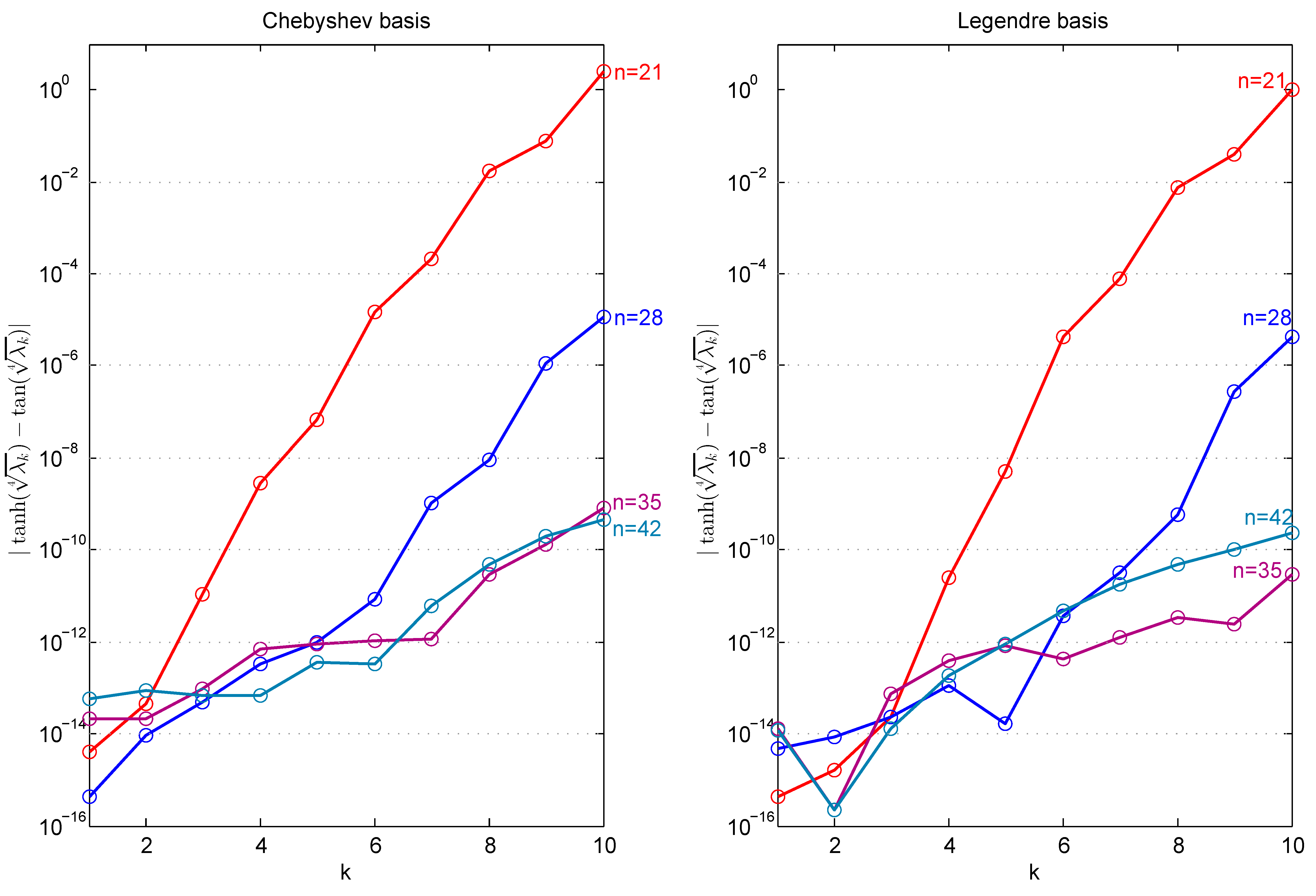
Example 1.
Consider the Sturm–Liouville boundary value problem
y ( 4 ) ( x ) = λ y ( x ) , 0 < x < 1 , y ( 0 ) = y ( 1 ) = y ( 0 ) = y ( 1 ) = 0 ,
whose exact eigenvalues satisfy [1,2]
tanh ( λ 4 ) tan ( λ 4 ) = 0 .
In that case D = N 4 λ I , where I is the identity matrix, and the boundary conditions can be represented by B n = [ v 0 ; v 1 ; v 0 N ; v 1 N 2 ] , where v 0 = [ 1 , 1 , , ( 1 ) n 1 ] and v 1 = [ 1 , 1 , , 1 ] are length n line vectors with the polynomial base values in the boundary domain.
For each n > 4 , C n in (7) is an n 4 square matrix and its determinant an n 4 degree polynomial. We use the Matlab function roots to find its zeros and we inspect their accuracy by testing if they satisfy relation (11).
In Figure 1, we present | tanh ( λ n , k 4 ) tan ( λ n , k 4 ) | for k = 1 , , 10 the first 10 eigenvalues approximations obtained with n = 21 , 28 , 35 and n = 42 , with Chebyshev and Legendre bases shifted to [ 0 , 1 ] .
Example 2.
A very similar problem, presented as the clamped rod problem in [12,18], is
y ( 4 ) ( x ) = λ y ( x ) , 1 < x < 1 , y ( ± 1 ) = y ( ± 1 ) = 0 .
In that case, and whenever we have a symmetric problem and a symmetric base, the matrix C n in (7) has zeros intercalating all non-zero elements. We can reduce the problem dimension, defining two matrices C O and C E with respectively the odd and the even entries of C n , then det ( C n ) = det ( C O ) det ( C E ) . In that case, since C n is an 4-upper Hessenberg matrix, C O and C E are 2-upper Hessenberg matrices. The sparsity pattern of those two matrices, in Legendre basis and with n = 52 , are showed in Figure 2.
The first 14 eigenvalues, evaluated with an 16 × 16 matrix, are presented in [12]. In Table 1, we compare those values with our results in the Legendre basis and with n = 16 and n = 52 . We present values of λ 52 , k / k 4 , which allows us to verify that our estimates satisfy the property that the kth eigenvalue is proportional to k 4 [18].
Example 3.
Consider the following Sturm–Liouville problem with non-null q and r coefficients
y ( 4 ) ( x ) ( α x 2 y ( x ) ) + ( β x 4 α ) y ( x ) = λ y ( x ) , 0 < x < 5 , y ( 0 ) = y ( 0 ) = y ( 5 ) = y ( 5 ) = 0 ,
with constants α , β R .
The operational matrix (9) for this case is
D = N 4 α M 2 N 2 2 α M N + β M 4 ( α + λ ) I
and B n = [ v 0 ; v 0 N 2 ; v 1 ; v 1 N 2 ] , with the same v 0 and v 1 vectors of the previous example.
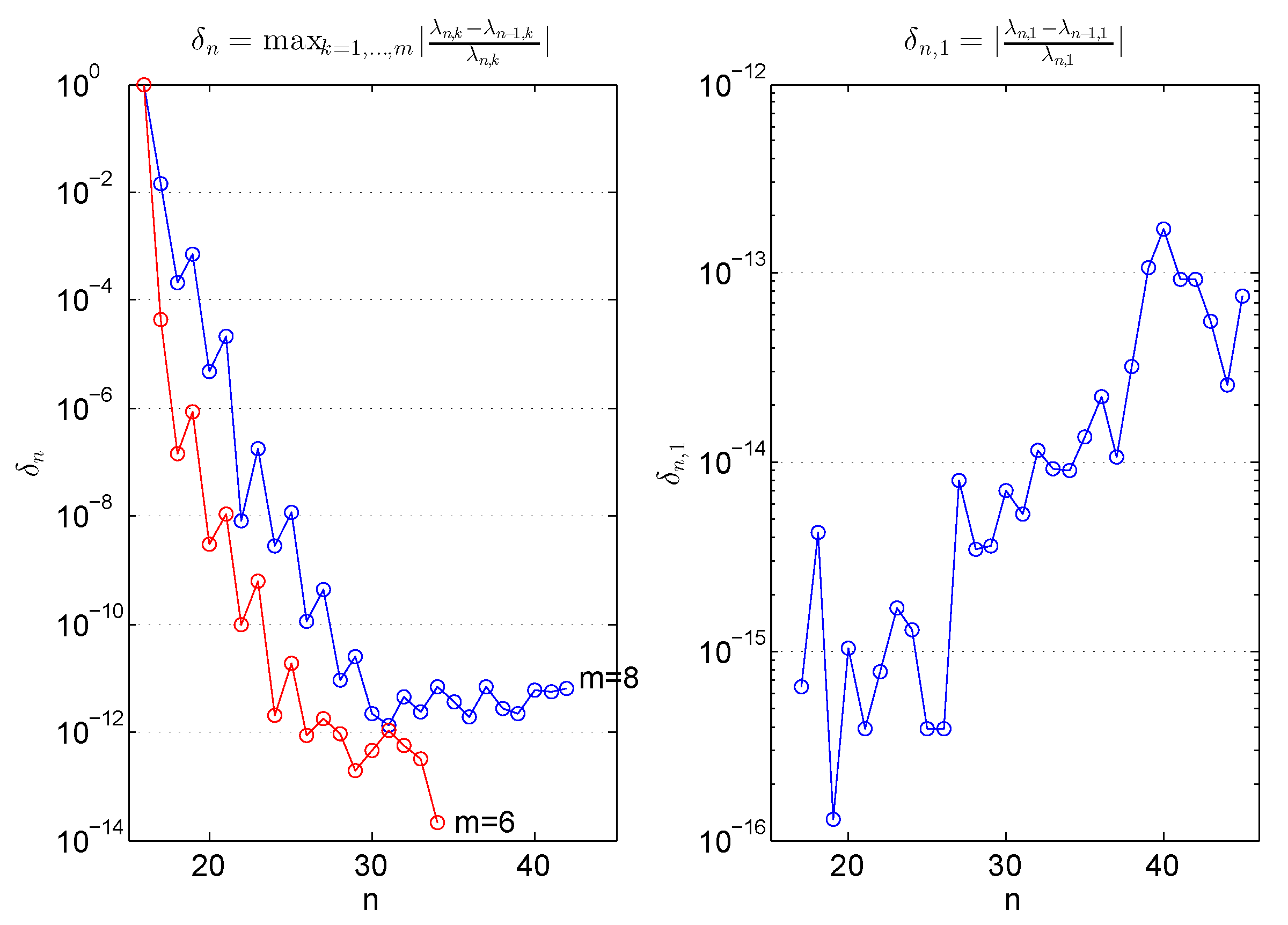
If λ n , k is the kth root of det ( T n ) , and considering δ ˜ n , k = λ n , k λ n 1 , k λ n , k as an estimative of the relative error in λ n 1 , k , then δ n = max k = 1 , , m | δ ˜ n , k | is an estimative of the maximum relative error in the first m eigenvalues of the problem. In Figure 3 left, we present δ n , with m = 6 and with m = 8 for Example 3 with α = 0.02 and β = 0.0001 for n = 16 , , 45 . In Figure 3 right, the absolute relative error | δ ˜ n , 1 | in the lowest eigenvalue is presented for the same n values.
In Table 2, we compare our results with those of [2] for the first six eigenvalues, and of [8] for the first 4, obtained with values α = 0.02 and β = 0.0001 .
Example 4.
Now, we consider the Orr–Sommerfeld problem
y ( 4 ) ( x ) 2 α 2 y + α 4 y = i α R [ ( U λ ) ( y α 2 y ) U y ] , 1 < x < 1 , y ( ± 1 ) = y ( ± 1 ) = 0 ,
with fixed constants α , R and function U.
The particular case U = 1 x 2 is the Poiseuille flow and, with α = 1 and R = 10000 was treated in [3,4,5,12]. The operational matrix in that case is
D = N 4 [ ( 2 α 2 + ( 1 λ ) i α R ) I i α R M 2 ] N 2 + ( α 4 + ( 1 λ ) i α 3 R 2 i α R ) I i α 3 R M 2 .
Like in Example 2, this is an upper Hessenberg matrix with zeros intercalating its non-zero elements and we can reduce the problem dimension, splitting in two matrices the Schur complement C n of the resulting Tau matrix T n . Choosing Chebyshev basis, this is the operational version of the Tau procedure of [5], where the author was confined to eigenvalues associated with symmetric eigenfunctions, which is equivalent to finding the eigenvalues of C E .
In [5], the author obtained for λ 1 = 0.23752649 + 0.00373967 i as an 8 decimal places exact value for the most unstable mode of this problem. Working with double-precision arithmetic, we obtain λ 1 = 0.2375264889204038 + 0.003739670740170985 i . This value results with n = 58 that is an 29 × 29 matrix C E , the same dimension used in [5].
In addition, with R c = 5772.22 , the smallest value of R for which an unstable eigenmode exists [5], and α c = 1.02056 , we get the results presented in Table 3, together with those of [5].

4. Non-Polynomial Coefficients

In the previous section, we solved problems in the conditions of Corollary 1, i.e., with differential operators acting in polynomial spaces. In a more general situation, if some of the coefficients p i in (6) are non-polynomial functions, then the corresponding matrices p i ( M ) are functions of M instead of polynomial expressions.
If a non-polynomial function p i in (6) can be defined implicitly by a differential problem, with polynomial coefficients, then we can first of all use the Tau method to find a polynomial approximation p ˜ i to p i and use p ˜ i ( M ) to approximate the matrix p i ( M ) .
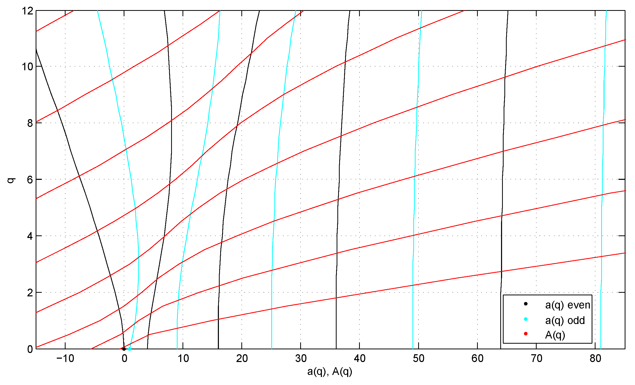
Example 5.
Mathieu’s equation appears related to wave equations in elliptic cylinders [19]. For an arbitrary parameter q, the problem is to find the values of λ for which non-trivial solutions of
y ( x ) + ( λ 2 q cos ( 2 x ) ) y ( x ) = 0
exist with prescribed boundary conditions.
It can be shown that there exists a countably infinite set of eigenvalues a r associated with even periodic eigenfunctions and a countably infinite set of eigenvalues b r associated with odd periodic eigenfunctions [19]. We are interested in reproducing some of those values given in there.
The operational matrix for problem (15) is
D = N 2 + λ I 2 q cos ( 2 M ) .
Our first step to approximate Mathieu’s eigenvalues is to approximate matrix cos ( 2 M ) . This can be done by, firstly, considering the function z ( x ) = cos ( 2 x ) as the solution of a differential problem, using Tau method to get a polynomial approximation z n ( x ) z ( x ) . In a second step, the operational matrix D is approximated by
D ˜ = N 2 + λ I 2 q z n ( M )
and, finally, the last step consists in building the Tau matrix T n and evaluating the zeros of its determinant.
We take integer values q = 0 , 1 , , 16 and boundary conditions y ( 1 ) = y ( π / 2 ) = 0 to get a r ( q ) for even r, y ( 1 ) = y ( π / 2 ) = 0 for odd r, and y ( 1 ) = y ( π / 2 ) = 0 to get b r ( q ) for odd r and y ( 1 ) = y ( π / 2 ) = 0 for even r.
In Figure 4, we show Mathieu eigenvalues a r ( q ) , r = 0 , , 5 and b r ( q ) , r = 1 , , 6 . Values were obtained with a 18th degree polynomial approximation z 18 cos ( 2 x ) and a 36 × 36 Tau matrix T 36 in Chebyshev polynomials.
We can observe, as pointed out in [19], that, for a fixed q > 0 , we have a 0 < b 1 < a 1 < b 2 < and that a r ( q ) , b r ( q ) approach r 2 as q approaches zero.
Example 6.
Mathieu’s equation also appears coupled with a modified Mathieu’s equation in systems of differential equations as multi parameter eigenvalues problems. The particular case
y 1 ( x 1 ) + ( λ 2 q cos ( 2 x 1 ) ) y 1 ( x 1 ) = 0 , 0 < x 1 < π 2 , y 1 ( 0 ) = y 1 ( π 2 ) = 0 , y 2 ( x 2 ) ( λ 2 q cosh ( 2 x 2 ) ) y 2 ( x 2 ) = 0 , 0 < x 2 < 2 , y 2 ( 0 ) = y 2 ( 2 ) = 0
is studied in [6,7] associated with the eigenfrequencies of an elliptic membrane with semi axes α = cosh ( 2 ) and β = sinh ( 2 ) .
To approximate eigenvalues for this problem, we first have to approximate cos ( 2 x ) and cosh ( 2 x ) by polynomials. Considering, as in the previous example, z 16 cos ( 2 x ) the 16th degree Tau solution of
z ( x ) + 4 z ( x ) = 0 , 0 < x < π 2 , z ( 0 ) = 1 , z ( π 2 ) = 1 ,
and w 16 cosh ( 2 x ) as the same degree Tau solution of
w ( x ) 4 w ( x ) = 0 , 0 < x < 2 , w ( 0 ) = 1 , w ( 0 ) = 0 ,
then
D ˜ 1 = N 2 + λ I 2 q z 16 ( M )
and
D ˜ 2 = N 2 λ I + 2 q w 16 ( M )
are matrices approximating the operational matrices associated with differential equations (16).
For each fixed q, we define matrices Tau T 1 and T 2 , representing Mathieu and modified Mathieu equations, respectively. Defining a n ( q ) the nth eigenvalue of T 1 , in ascending order, and A m ( q ) the mth eigenvalue of T 2 , in descending order, in [6], it was proved that a n ( q ) and A m ( q ) are analytical functions of q. Moreover, for each pair ( m , n ) , it was proved the existence and uniqueness of an intersection point of curves a n ( q ) and A m ( q ) . Those intersections identify the eigenmodes of the elliptic membrane.
In Figure 5, we recover, and extend, figures presented in [6] and in [7]. Intersection points of a n ( q ) , the almost vertical curves, and A m ( q ) , the oblique curves, are the eigenpairs ( a , q ) of (16).

5. Nonlinear Eigenvalues Problem

In some differential problems, the eigenvalues can arise in a nonlinear relation with eigenfunctions. Let us consider the following second order problem, related to Weber’s equation:
Example 7.
y ( x ) + ( λ + λ 2 x 2 ) y ( x ) = 0 , 1 < x < 1 , y ( 1 ) = y ( 1 ) = 0 .
The operational matrix corresponding to the differential equation is
D = N 2 + λ I + λ 2 M 2
and so det ( T n ) is a polynomial with degree 2 ( n 2 ) in λ .
In Table 4, we present the 10 eigenvalues closest to zero, obtained with n = 30 and with n = 31 . We can verify that max k = 5 , , 5 | λ k ( 30 ) λ k ( 31 ) | < 5 × 10 9 .

6. Conclusions

Since the pioneering works of Orzag [5] and Ortiz and Samara [9], the Tau method has been scarcely used to solve differential eigenvalues’ problems. With our work, we conclude that the Tau method is a competitive one if we want to evaluate with high accuracy the first eigenvalues, in a large kind of differential problem.

Author Contributions

Formal analysis, J.M.A.M. and M.J.R.; Investigation, J.M.A.M. and M.J.R.; Writing—original draft, J.M.A.M. and M.J.R.; Writing—review and editing, J.M.A.M. and M.J.R.

Funding

This research was partially supported by CMUP (UID/ MAT/ 00144/ 2019), which is funded by FCT (Portugal) with national (MEC) and European structural funds through the programs FEDER, under the partnership agreement PT2020.

Conflicts of Interest

The authors declare no conflict of interest.

References

  1. Attili, B.S.; Lesnic, D. An efficient method for computing eigenelements of Sturm–Liouville fourth-order boundary value problems. Appl. Math. Comput. 2006, 182, 1247–1254. [Google Scholar] [CrossRef]
  2. Farzana, H.; Islam, M.S.; Bhowmik, S.K. Computation of Eigenvalues of the Fourth Order Sturm–Liouville BVP by Galerkin Weighted Residual Method. J. Adv. Math. Comput. Sci. 2015, 9, 73–85. [Google Scholar] [CrossRef] [PubMed]
  3. Reddy, S.C.; Schmid, P.J.; Henningson, D.S. Pseudospectra of the Orr–Sommerfeld Operator. SIAM J. Appl. Math. 1993, 53, 15–47. [Google Scholar] [CrossRef]
  4. Pop, I.S.; Gheorghiu, C.I. A Chebyshev–Galerkin Method for Fourth Order Problems. In Proceedings of the International Conference on Approximation and Optimization, Cluj-Napoca, Romania, 29 July–1 August 1996. [Google Scholar]
  5. Orzag, S.A. Accurate solution of the Orr–Sommerfeld stability equation. J. Fluid Mech. 1971, 50, 689–703. [Google Scholar] [CrossRef]
  6. Neves, A. Eigenmodes and eigenfrequencies of vibrating elliptic membranes: A Klein oscillation theorem and numerical calculations. Commun. Pure Appl. Anal. 2009, 9, 611–624. [Google Scholar] [CrossRef]
  7. Gheorghiu, C.I.; Hochstenbach, M.E.; Plestenjak, B.; Rommes, J. Spectral collocation solutions to multiparameter Mathieu’s system. Appl. Math. Comput. 2012, 218, 11990–12000. [Google Scholar] [CrossRef]
  8. Chanane, B. Accurate solutions of fourth order Sturm–Liouville problems. J. Comput. Appl. Math. 2010, 234, 3064–3071. [Google Scholar] [CrossRef]
  9. Ortiz, E.L.; Samara, H. Numerical solution of differential eigenvalue problems with an operational approach to the Tau method. Computing 1983, 31, 95–103. [Google Scholar] [CrossRef]
  10. Matos, J.M.A.; Rodrigues, M.J.; Matos, J.C. Explicit formulae for derivatives and primitives of orthogonal polynomials. arXiv 2017, arXiv:1703.00743v2. [Google Scholar]
  11. Matos, J.M.A.; Rodrigues, M.J.; Matos, J.C. Explicit Formulae for Intergral-Differential Operational Matrices. submitted for publication. 2019. [Google Scholar]
  12. Gheorghiu, C.I. Spectral Methods for Differential Problems; Institute of Numerical Analysis: Cluj-Napoca, Romania, 2007. [Google Scholar]
  13. Charalambides, M.; Waleffe, F. Gegenbauer Tau Methods with and without Spurious Eigenvalues. SIAM J. Numer. Anal. 2008, 47, 48–68. [Google Scholar] [CrossRef]
  14. Trindade, M.; Matos, J.; Vasconcelos, P.B. Towards a Lanczos Tau-Method Toolkit for Differential Problems. Math. Comput. Sci. 2016, 10, 313–329. [Google Scholar] [CrossRef]
  15. Trindade, M.; Matos, J.; Vasconcelos, P.B. Dealing with functional coefficients within Tau method. Math. Comput. Sci. 2018, 12, 183–195. [Google Scholar] [CrossRef]
  16. Vasconcelos, P.B.; Matos, J.; Trindade, M.S. Spectral Lanczos’ Tau Method for Systems of Nonlinear Integro-Differential Equations. In Integral Methods in Science and Engineering, Volume 1: Theoretical Techniques; Constanda, C., Dalla Riva, M., Lamberti, P.D., Musolino, P., Eds.; Springer: Cham, Switzerland, 2017; pp. 305–314. [Google Scholar]
  17. Chihara, T.S. An Introduction to Orthogonal Polynomials; Dover Publications: Mineola, NY, USA, 2011. [Google Scholar]
  18. Funaro, D.; Heinrichs, W. Some Results About the Pseudospectral Approximation of One-Dimensional Fourth-Order Problems. Numer. Math. 1990, 58, 399–418. [Google Scholar] [CrossRef]
  19. Blanch, G. Mathieu Functions. In Handbook of Mathematical Functions; Abramowitz, M., Stegun, I.A., Eds.; Dover Publications: Mineola, NY, USA, 1974; pp. 721–750. [Google Scholar]
Figure 1. | tanh ( λ n , k 4 ) tan ( λ n , k 4 ) | , k = 1 , 2 , , 10 , λ n , k being the roots of det ( T n ) in Example 1.
Mca 24 00096 g001
Figure 2. Sparsity pattern of C O and C E with n = 48 in Legendre base, for Example 2.
Mca 24 00096 g002
Figure 3. δ n = max k = 1 , , m δ ˜ n , k , m = 6 and m = 8 , (left) and δ n , 1 (right), in Example 3.
Mca 24 00096 g003
Figure 4. Mathieu eigenvalues a r ( q ) , r = 0 , , 5 and b r ( q ) , r = 1 , , 6 , for q = 0 , , 16 in Example 5.
Mca 24 00096 g004
Figure 5. Mathieu eigenvalues a n ( q ) and A m ( q ) , for q = 0 , , 12 in Example 5. Only values a ( q ) , A ( q ) [ 15 , 85 ] are presented.
Mca 24 00096 g005
Table 1. Eigenvalues of Example 2 presented in [12] and λ n , k with n = 20 and n = 52 in Legendre basis.
k λ k [12] λ 16 , k λ 52 , k λ 52 , k / k 4
13.12852439 × 10 1 3.128524385877707 × 10 1 3.128524385877221 × 10 1 31
22.377210675 × 10 2 2.377210675311160 × 10 2 2.377210675311198 × 10 2 15
39.136018866 × 10 2 9.136018831954221 × 10 2 9.136018831951466 × 10 2 11
42.4964874758 × 10 3 2.496487437857343 × 10 3 2.496487437856835 × 10 3 9.8
55.5710074688 × 10 3 5.570962978086419 × 10 3 5.570962978573987 × 10 3 8.9
61.08631975968 × 10 4 1.086758221396396 × 10 4 1.086758221697812 × 10 4 8.4
71.93928004466 × 10 4 1.926303581823010 × 10 4 1.926302825661405 × 10 4 8.0
83.05369477203 × 10 4 3.178016789424974 × 10 4 3.178009645408997 × 10 4 7.8
96.03075735206 × 10 4 4.960468438481630 × 10 4 4.958769590877672 × 10 4 7.6
107.11035649235 × 10 4 7.407231618213559 × 10 4 7.400084934912209 × 10 4 7.4
113.597677558196 × 10 5 1.091110089932048 × 10 5 1.064806931408837 × 10 5 7.3
123.856105241227 × 10 5 1.548144789089380 × 10 5 1.486344772858071 × 10 5 7.2
131.62401642422808 × 10 7 2.619042084314734 × 10 5 2.022155654215451 × 10 5 7.1
141.71337968904269 × 10 7 3.728032882888538 × 10 5 2.691234348268295 × 10 5 7.0
Table 2. Eigenvalues of Example 3 presented in [8] and [2] and λ n , k with n = 35 .
k λ k [8] λ k [2] λ n , k
10.215050864370.215050864369714920.2150508643697136
22.754809934682.7548099346828842.754809934683077
313.215351540613.21535154055881213.21535154055782
440.950819348740.9508197591375540.95081975916199
5 99.0534781381388099.05347806349896
6 204.35449348957833204.3557322681771
Table 3. Values of λ 1 of Example 4 with critical values R c = 5772.22 and α = 1.02056 .
n λ 1
50 0.2640017404987603 3.099641201518763 i × 10 9
60 0.2640017396216782 3.035288544655118 i × 10 9
80 0.2640017390806805 2.028898296212456 i × 10 9
n λ 1 [5]
44 0.26400174 1.7 i × 10 9
50 0.26400174 + 5.9 i × 10 10
Table 4. Eigenvalues of Example 7 with n = 30 and n = 31 . Decimal places presented are those that coincide, until to the first distinct two.
k λ k ( n = 30 ) λ k ( n = 31 )
5 19.674904478 19.674904482
4 13.62505355977 13.62505355969
3 13.200062264051 13.200062264066
2 7.0356879747644 7.0356879747642
1 6.59716200235713 6.59716200235723
11.9517023649903291.951702364990324
24.286111061180164.28611106118021
37.54592033499917.5459203349981
410.12600591595910.126005915966
513.5287021742613.52870217408

