Adaptive Control of Resistance Spot Welding Based on a Dynamic Resistance Model

Abstract

Resistance spot welding is a process commonly used for joining a stack of two or three metal sheets at desired spots. Such welds are accomplished by holding the metallic workpieces together by applying pressure through the tips of a pair of electrodes and then passing a strong electric current for a short duration. This kind of welding process often suffers from two common drawbacks, namely, inconsistent weld quality and inadequate nugget size. In order to address these problems, a new theoretical approach of controlling resistance spot welding processes is proposed in this paper. The proposed controller is based on a simplified dynamical model of the resistance spot welding process and employs the principle of adaptive one-step-ahead control. It is essentially an adaptive tracking controller that estimates the unknown process parameters and adjusts the welding voltage continuously to make sure that the nugget resistance tracks a desired reference resistance profile. The modeling and controller design methodologies are discussed in detail. Also, the results of a simulation study to evaluate the performance of the proposed controller are presented. The proposed control scheme is expected to reduce energy consumption and produce consistent welds.

1. Introduction

Resistance spot welding (RSW) is an electrothermal process in which contacting metal surfaces are joined by heat. The metal surfaces are held together under pressure exerted by two electrodes. The heat needed to create the weld is generated by applying a strong electric current through the electrodes and the workpieces, as shown in Figure 1. The welding process is related to the metallurgy of the materials involved in welding, including the base metal and the electrodes [1]. The flow of a strong electric current through the metal sheets causes heating due to the resistance of the joining surfaces and the sheets. Most of the heating is concentrated near the faying surface, since the contact resistance is very high compared to the bulk resistance of the sheets, causing melting and formation of a weld nugget. Depending on the thickness and type of material, welding current ranges from 1000 to 20,000 amperes, or even higher, while the voltage typically lies between 1 and 30 volts [2].

A resistance spot welding cycle consists of three main stages as follows:

Stage 1:

Squeeze time, during which pressure is applied by the electrodes to squeeze the workpieces.

Stage 2:

Welding time, during which a high current is applied, causing melting and formation of a nugget.

Stage 3:

Hold time, during which pressure is maintained after the welding current is ceased, to allow cooling of the nugget and prevent cracks.

The resistance spot welding process is used in many different industries, including automotive, aerospace, railway, military, and industrial manufacturing. It is the most popular welding technology used by the automotive industry to weld various sheet metals to form the chassis and body of a vehicle. About 4000–6000 spot welds are used to manufacture a typical automotive vehicle today. Considering a worldwide annual production volume of 80 million automotive vehicles, an energy efficient RSW controller can result in significant energy savings and reduce carbon footprint accordingly.

RSW welding often suffers from two common drawbacks, namely, inconsistent weld quality and inadequate nugget size. In order to address these problems, a number of remedies have been proposed. These include monitoring and control of welding parameters to improve weld quality. Some of the conventional RSW control techniques proposed to date include proportional-integral (PI) [3], proportional-derivative (PD) [4], proportional-integral-derivative (PID) [5], fuzzy [6,7,8], neural networks [9,10], or a combination of fuzzy and neural networks [11]. One of the main drawbacks of these techniques stems from the fact they do not take into consideration the thermal dynamics of an RSW process. Also, most of these systems do not take into account any changes in process parameters. Some of the recently proposed RSW control methods address the above drawbacks by proposing either model-based or adaptive controllers. These include a power reference-based controller [12], intelligent hysteresis and PI controllers [13], and an adaptive power and current controller to reduce shunting effects [14].

As a remedy to some of the shortcomings of the existing methodologies, a new RSW control design method based on using dynamic resistance as a feedback signal is proposed in this paper. Although the idea of using dynamic resistance signature for monitoring quality of RSW welds has been investigated by a number of researchers over past three decades [15,16,17,18,19,20], the idea of using it as a feedback signal for controlling an RSW process is relatively new. Although this idea was introduced by a number of researchers, such as [17,21], no methods of actually doing it were presented. However, a method of doing it using model predictive control (MPC) was proposed in [22]. It introduces the idea of a dynamic resistance tracking controller, which is conceptually similar to the controller proposed in this paper. However, the RSW resistance model developed there is an empirical dynamical resistance model consisting of three first order exponential curves to emulate the characteristics of the resistance of the workpiece during the heating, melting, and cooling phases, respectively. It proposes a model predictive controller (MPC) based on the above simplistic empirical model, but judging from the results presented, it does not seem to perform well.

As mentioned earlier, an RSW controller design based on using dynamic resistance as a feedback signal is proposed in this paper. It is based on a dynamic resistance model of the RSW process, which is slightly different from the thermal RSW process models investigated in [23,24]. The main drawback of using a thermal model for RSW control has to do with the difficulty of directly monitoring the nugget temperature, which is why an indirect monitoring scheme based on measurement of the dynamic resistance was suggested in [23,24]. The above difficulty is avoided here by developing and utilizing a dynamic resistance model of the RSW process. The development of such a model starts from a simplified heat balance model of an RSW process proposed in [23,24,25], which is then converted into a dynamical resistance model using a nonlinear relationship between temperature and resistance. The resulting model governs the variation of workpiece resistance during welding time. Next, an adaptive one-step-ahead (AOSA) controller is designed based on the above model. The proposed adaptive controller estimates the model parameters and generates a control signal based on the estimated parameters, which enable the workpiece resistance to follow a desired reference resistance profile. Simulation results show that an AOSA controller is capable of tracking a reference resistance profile when the welding parameters are unknown, as well as reducing the energy required to make a weld.

The organization of this paper is as follows. Section 2 presents modeling of an RSW nugget formation process. The development of a dynamical resistance model and its validation are discussed in Section 3. The design of an adaptive controller is discussed in Section 4. Section 5 presents the results of some simulation studies, and finally, some concluding remarks are provided in Section 6.

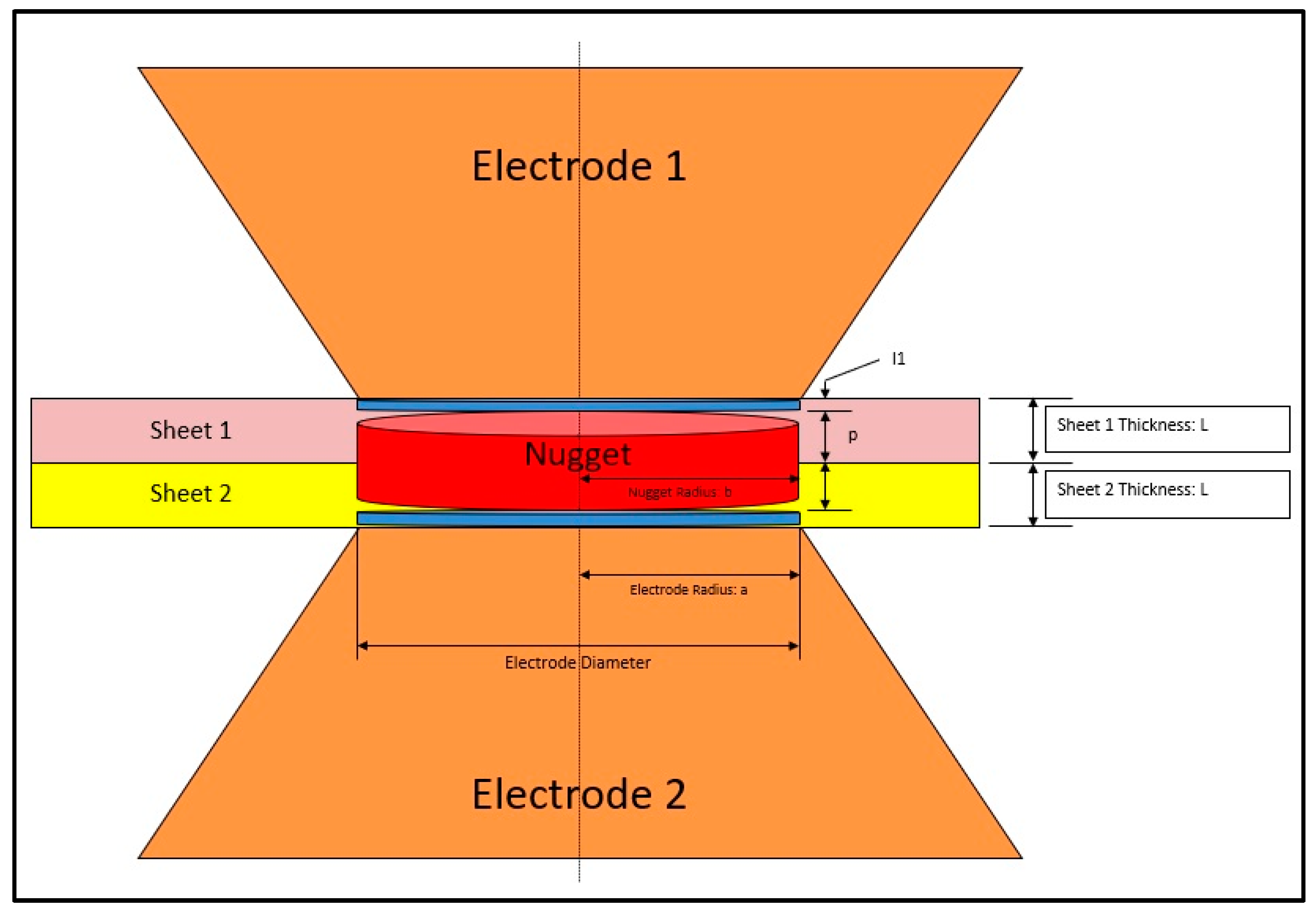
2. Modeling of an RSW Nugget Formation Process

This section presents a dynamical resistance model of the RSW process. First, a simplified heat balance model of the process is described, and then it is converted to a dynamical resistance model.

Electro-Thermal Dynamical Model of an RSW Nugget Formation Process

Following the footsteps of [23,24,25], the development of an electro-thermal model is started from a simplified RSW nugget model, shown in Figure 2 below. The heat balance equations for this model can be developed as follows.

The total heat generation rate, ${\dot{Q}}_g\left(t\right)$, is given by:

$${\dot{Q}}_g\left(t\right)=\frac{V^2\left(t\right)}{R\left(t\right)}$$

(1)

where $V\left(t\right)$ denotes the welding voltage and $R\left(t\right)$is the total workpiece resistance, which can be described by:

$$R\left(t\right)=R_w\left(t\right)+R_c\left(t\right)+R_e\left(t\right).$$

(2)

Here, $R_w\left(t\right)$ denotes the bulk resistance of the workpieces,$R_c\left(t\right)$ represents the total contact resistance, and $R_e\left(t\right)$ denotes the electrode resistance. Since $R_e$ is very small compared to the other two components, it can be neglected in (2). It may be noted that for a two-stack workpiece, the total resistance can also be rewritten as:

$$R\left(t\right)\approx 2R{\left(t\right)}_{electrode-sheet}+R{\left(t\right)}_{sheet-sheet}+R_w\left(t\right)$$

(3)

The heat of fusion required for nugget formation is given by:

$$H_f=H{V}_n,$$

(4)

where $H$denotes the heat of fusion per unit volume and $V_n$ denotes the nugget volume, which is given by:

$$V_n=2\pi a^{2}p,$$

(5)

where $p$ and$a$ are the penetration radius and nugget radius, respectively. Substitution of (5) into (4) and normalization over the weld duration,$\Delta t$, yields:

$$c_1=\frac{H_f}{\Delta t}=2H\pi a^{2}p.$$

(6)

Neglecting the heat loss to the surroundings and the electrodes, the heat required to raise the temperature of the nugget by $d\theta \left(t\right)$is given by:

$$d{Q}_T\left(t\right)=\rho C_p{V}_{n}d\theta \left(t\right),$$

(7)

$$=c_{2}d\theta \left(t\right),$$

(8)

where

$$c_2=\rho C_{p}2\pi a^{2}p,$$

(9)

and $\rho$ denotes the density,$C_p$ is the specific heat, and $d\theta \left(t\right)$ denotes the temperature rise.

Next, the total heat loss rate is given by:

$${\dot{Q}}_L\left(t\right)={\dot{Q}}_a\left(t\right)+{\dot{Q}}_r\left(t\right)$$

(10)

where ${\dot{Q}}_a\left(t\right)$ and ${\dot{Q}}_r\left(t\right)$ denote the axial and radial heat loss rates, respectively. Inserting their mathematical expressions, details of which can be found in [24,25,26], gives:

$$\begin{array}{c}{\dot{Q}}_L\left(t\right)=k_1\pi a^2\left[\frac{\theta \left(t\right)-{\theta }_I}{l_1}+\frac{10\theta \left(t\right)\beta L}{b\sqrt{\alpha }}\right]\\ =\left[\frac{k_1\pi a^2}{l_1}+\frac{10k_1\pi a^2\beta L}{b\sqrt{\alpha }}\right]\theta \left(t\right)-\frac{k_1\pi a^2{\theta }_I}{l_1}\\ =c_3\theta \left(t\right)-c_4\end{array}$$

(11)

where

$$c_3=\left[\frac{k_1\pi a^2}{l_1}+\frac{10k_1\pi a^2\beta L}{b\sqrt{\alpha }}\right],$$

(12)

$$c_4=\frac{k_1\pi a^2{\theta }_I}{l_1}.$$

(13)

In the above equations, $k_1$ denotes the thermal conductivity, $a$ is the nugget radius, and $\theta \left(t\right)$ and ${\theta }_I$ represent the melting temperature and the interface temperature of the workpieces, respectively. Also, $l_1$is the distance from the melting interface to the electrodes contact area, $\beta$represents the final penetration to workpiece thickness ratio, $L$ is the sheet thickness, $b$ represents the electrode radius, and $\alpha$ denotes the thermal diffusivity of the workpiece. Also, to avoid complexity of the model, the thermal conductivity and the thermal diffusivity are assumed to be constants.

The heat balance equation over the time interval, (t, t + dt), is given by:

$${\dot{Q}}_g\left(t\right)=\frac{H_f}{\Delta t}dt+d{Q}_T\left(t\right)+{\dot{Q}}_L\left(t\right)dt.$$

(14)

Substituting (1), (6), (8), and (11) in (14) and rearranging it, gives:

$$c_2\frac{d\theta \left(t\right)}{dt}=\frac{V^2\left(t\right)}{R\left(t\right)}-c_3\theta \left(t\right)+c_4-c_1$$

(15)

or equivalently,

$$\frac{d\theta \left(t\right)}{dt}=c_5\frac{V^2\left(t\right)}{R\left(t\right)}-c_6\theta \left(t\right)+c_7$$

(16)

where

$$c_5=\raisebox{1ex}{$1$}\!\left/ \!\raisebox{-1ex}{$c_2$}\right.,$$

(17)

$$c_6=\raisebox{1ex}{$c_3$}\!\left/ \!\raisebox{-1ex}{$c_2$}\right.,$$

(18)

$$c_7=\left(c_4-c_1\right)/c_2$$

(19)

Equation (16) represents a simplified electro-thermal dynamical model of the RSW process. From this, a dynamical resistance model is developed as follows.

3. Dynamical Resistance Model of an RSW Nugget Formation Process

The development of a dynamical resistance model exploits the functional relationship between resistance and temperature. To start with, it is assumed that $R\left(t\right)$ can be approximately represented by:

$$R\left(t\right)=R_{°}\left[1+\alpha \left(\theta \right)\left(\theta \left(t\right)-{\theta }_{°}\right)\right],$$

(20)

where $\alpha \left(\theta \right)$ denotes the temperature coefficient of resistance, and $R_{°}$ is the resistance at room temperature,${\theta }_{°}$.

Equivalently, one can write:

$$\theta \left(t\right)=\beta \left(\theta \right)\left(R\left(t\right)-R_{°}\right)+{\theta }_{°}$$

(21)

where

$$\beta \left(\theta \right)=\frac{1}{\alpha \left(\theta \right)R_{°}}$$

(22)

Differentiation of (21) yields:

$$\frac{d\theta \left(t\right)}{dt}=\beta \left(\theta \right)\frac{dR\left(t\right)}{dt}+\gamma \left(\theta \right)\left(R\left(t\right)-R_{°}\right)$$

(23)

where

$$\gamma \left(\theta \right)=\frac{d\beta \left(\theta \right)}{dt}.$$

(24)

Substitution of (16) in (23) gives:

$$\beta \left(\theta \right)\frac{dR\left(t\right)}{dt}+\gamma \left(\theta \right)\left(R\left(t\right)-R_{°}\right)=c_5\frac{V^2\left(t\right)}{R\left(t\right)}-c_6\left[\beta \left(\theta \right)\left(R\left(t\right)-R_{°}\right)+{\theta }_{°}\right]+c_7.$$

(25)

Also, re-arrangement of the above equation yields:

$$\frac{dR\left(t\right)}{dt}=c_8\frac{V^2\left(t\right)}{R\left(t\right)}-c_{9}R\left(t\right)+c_{10}\left(t\right),$$

(26)

where

$$c_8\left(t\right)=\raisebox{1ex}{$c_5$}\!\left/ \!\raisebox{-1ex}{$\beta \left(\theta \right)$}\right.,$$

(27)

$$c_9\left(t\right)=\frac{\gamma \left(\theta \right)}{\beta \left(\theta \right)}+c_6,$$

(28)

$$c_{10}\left(t\right)=\frac{\gamma \left(\theta \right)}{\beta \left(\theta \right)}{R}_{°}+\frac{c_7}{\beta \left(\theta \right)}-\frac{c_6{\theta }_{°}}{\beta \left(\theta \right)}+c_6{R}_{°}$$

(29)

In Equations (27)–(29), the parameters $c_8$, $c_9$ and $c_{10}$ are assumed to vary with time since $\beta \left(\theta \right)$ and $\gamma \left(\theta \right)$ vary with time (as a result of variation of $\theta$ with time).

Finally, for the sake of notational convenience, let $y\left(t\right)=R\left(t\right)$ and $u\left(t\right)=V\left(t\right)$. Then (26) can be rewritten as:

$$\frac{dy\left(t\right)}{dt}=c_8\left(t\right)\frac{u^2\left(t\right)}{y\left(t\right)}-c_9\left(t\right)y\left(t\right)+c_{10}\left(t\right)$$

(30)

Using a first order Euler approximation for $\frac{dy}{dt}$ with a sampling period, $T_s$, Equation (30) yields the following discrete time system:

$$\frac{y\left(k+1\right)-y\left(k\right)}{T_s}=c_8\left(k\right)\frac{u^2\left(k\right)}{y\left(k\right)}-c_9\left(k\right)y\left(k\right)+c_{10}\left(k\right)$$

(31)

or equivalently,

$$y\left(k+1\right)=A\left(k\right)y\left(k\right)+B\left(k\right)\frac{u^2\left(k\right)}{y\left(k\right)}+C\left(k\right)$$

(32)

where

$$A\left(k\right)=1-c_9\left(k\right)T_s,$$

(33)

$$B\left(k\right)=c_8\left(k\right)T_s,$$

(34)

$$C\left(k\right)=c_{10}\left(k\right)T_s,$$

(35)

and $k$ is the discrete time index $\left(k=0, 1, 2, \dots \right),$ with $k{T}_s$ denoting the sampling instances.

Equation (32) represents a dynamical resistance model of the RSW process, which is characterized by three unknown time-varying parameters, A(k), B(k), and C(k). The validation of this model is discussed in the next subsection.

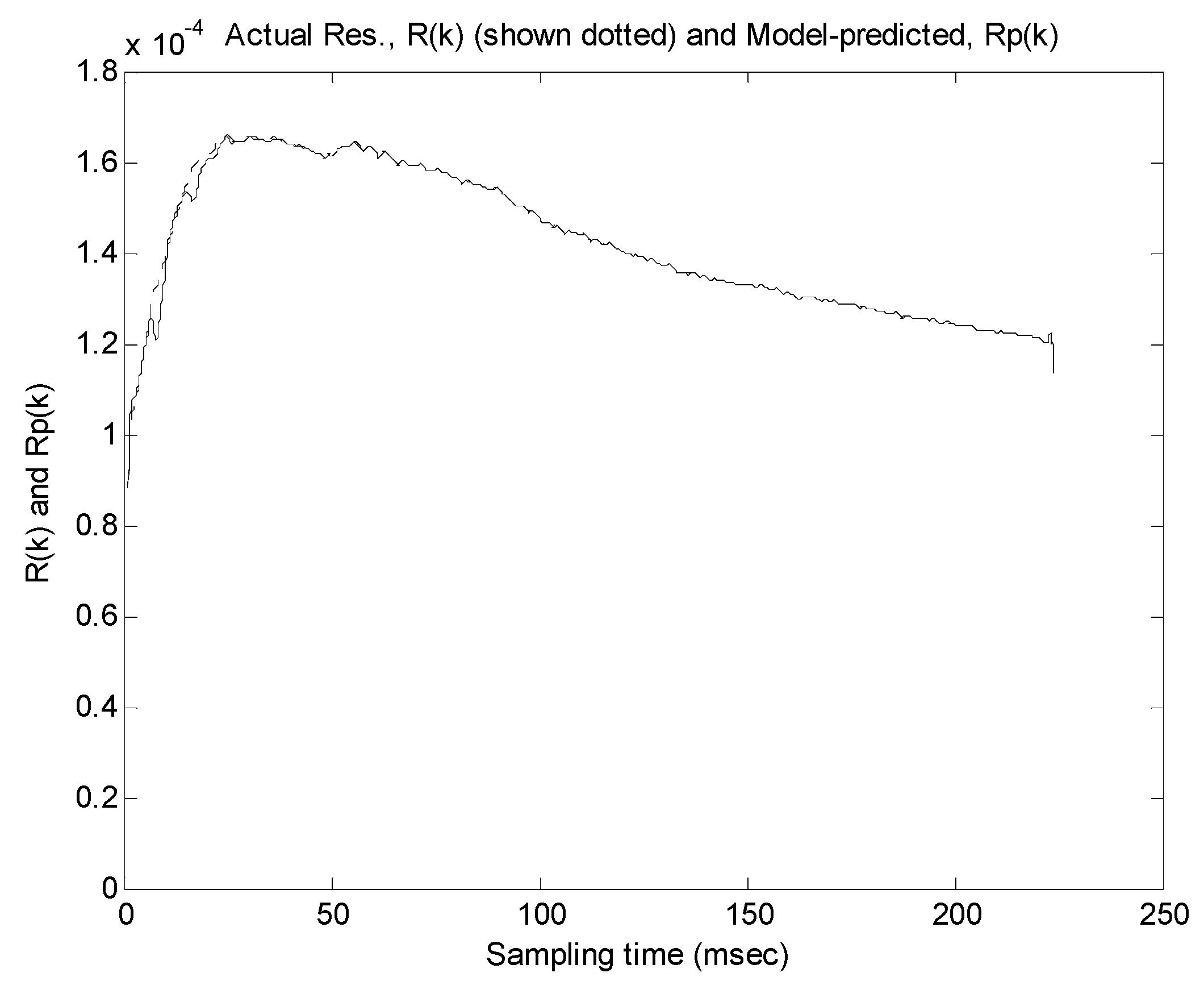
Validation of the Dynamic Resistance Model

The validation of the above dynamic resistance model requires voltage and current data from an adaptive weld controller that uses feedback signals to adjust its welding voltage with time. A set of voltage–current data collected from a constant heat controller (CHC) [26], manufactured by Welding Technology Corporation, is used for this purpose.

Figure 3 shows the welding voltage samples, V(k), and welding current samples, I(k), collected during a spot weld performed by a CHC machine. The dynamic resistance, R(k), is calculated from the above data by simply dividing V(k) by I(k) at each sample time, k. Then, a recursive least squares parameter estimation algorithm, described in Section 4.1 below, is used to estimate the parameters, A(k), B(k), and C(k), of the above dynamic resistance model. These estimated model parameters are shown in Figure 4.

Finally, in order to assess the goodness of fit of the proposed model, the estimated model parameters, $\widehat{A}\left(k\right), \widehat{B}\left(k\right),$and $\widehat{C}\left(k\right)$, are next used to compute the predicted resistance values, R_p(k), at each sample point, k. The goodness of fit between actual resistance, R(k), and the model-predicted resistance, R_p(k), is shown in Figure 5, which demonstrates the validity of the above model. It may be pointed out that similar results were also obtained from other CHC welding data.

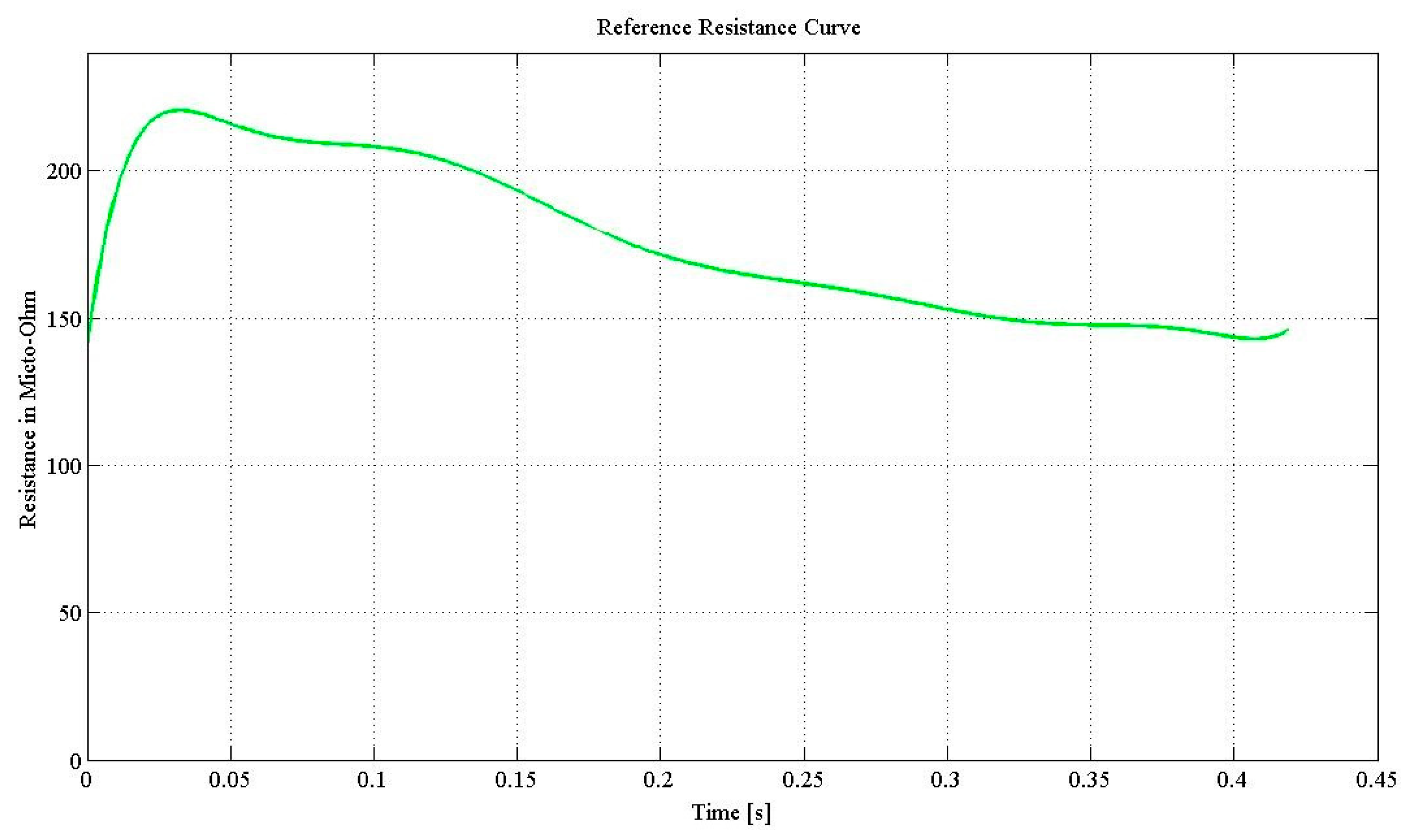
4. Design of an Adaptive RSW Controller

Since the system represented by Equation (32) is characterized by time-varying parameters, an adaptive controller would be an appropriate tool for controlling such a system. However, the nonlinear nature of the above system precludes usage of a conventional linear adaptive controller. In view of above, an adaptive one-step-ahead controller is proposed to be used here. The three key steps required to implement such a controller involve measurement of the input (welding voltage) and output (dynamic resistance) at uniform sampling intervals, estimation of the dynamic resistance model parameters, $\widehat{A}\left(k\right), \widehat{B}\left(k\right),$and $\widehat{C}\left(k\right)$, using a recursive parameter estimation algorithm, such as recursive least squares (RLS), and computation of a control signal based on the estimated parameter values. The estimation of model parameters and computation of a control signal are discussed in the following subsections.

4.1. Parameter Estimation

First, the model Equation (32) is rewritten in the following predictive form:

$$y\left(k+1\right)=\phi {\left(k\right)}^T{X}^{*}$$

(36)

where

$$\phi \left(k\right)={\left[\begin{array}{ccc}y\left(k\right)& \frac{u^2\left(k\right)}{y\left(k\right)}& 1\end{array}\right]}^T,$$

(37)

$$X^{*}={\left[\begin{array}{ccc}A& B& C\end{array}\right]}^T.$$

(38)

Here, $X$ denotes the vector of unknown system parameters that are estimated recursively using the following RLS algorithm:

$$\widehat{X}\left(k\right)=\widehat{X}\left(k-1\right)+\frac{P\left(k-2\right)\phi \left(k-1\right)}{\lambda +\phi {\left(k-1\right)}^{T}P\left(k-2\right)\phi \left(k-1\right)}\left[y\left(k\right)-\phi {\left(k-1\right)}^T\widehat{X}\left(k-1\right)\right]; k\ge 1,$$

(39)

$$P\left(k-1\right)=\left(\frac{1}{\lambda }\right)[P\left(k-2\right)-\frac{P\left(k-2\right)\phi \left(k-1\right)\phi {\left(k-1\right)}^{T}P\left(k-2\right)}{1+\phi {\left(k-1\right)}^{T}P\left(k-2\right)\phi \left(k-1\right)}],$$

(40)

$$\widehat{X}\left(0\right)={\left[\begin{array}{ccc}0& \epsilon & 0\end{array}\right]}^T,$$

(41)

$$P\left(-1\right)=\sigma I,$$

(42)

where λ, 0 < λ < 1, denotes a forgetting factor,$\epsilon >0$ is a small number, and $\widehat{B}\left(k\right)$ is always constrained to be non-negative, i.e.,

$$\widehat{B}\left(k\right)\ge \epsilon >0 \mathrm{for}\mathrm{all}k.$$

(43)

Furthermore, since $\widehat{X}\left(k\right)$ denotes an estimate of$X^{*}$, the predicted output at time $k+1$ is defined as:

$$\widehat{y}\left(k+1\right)=\phi {\left(k\right)}^T\widehat{X}\left(k\right).$$

(44)

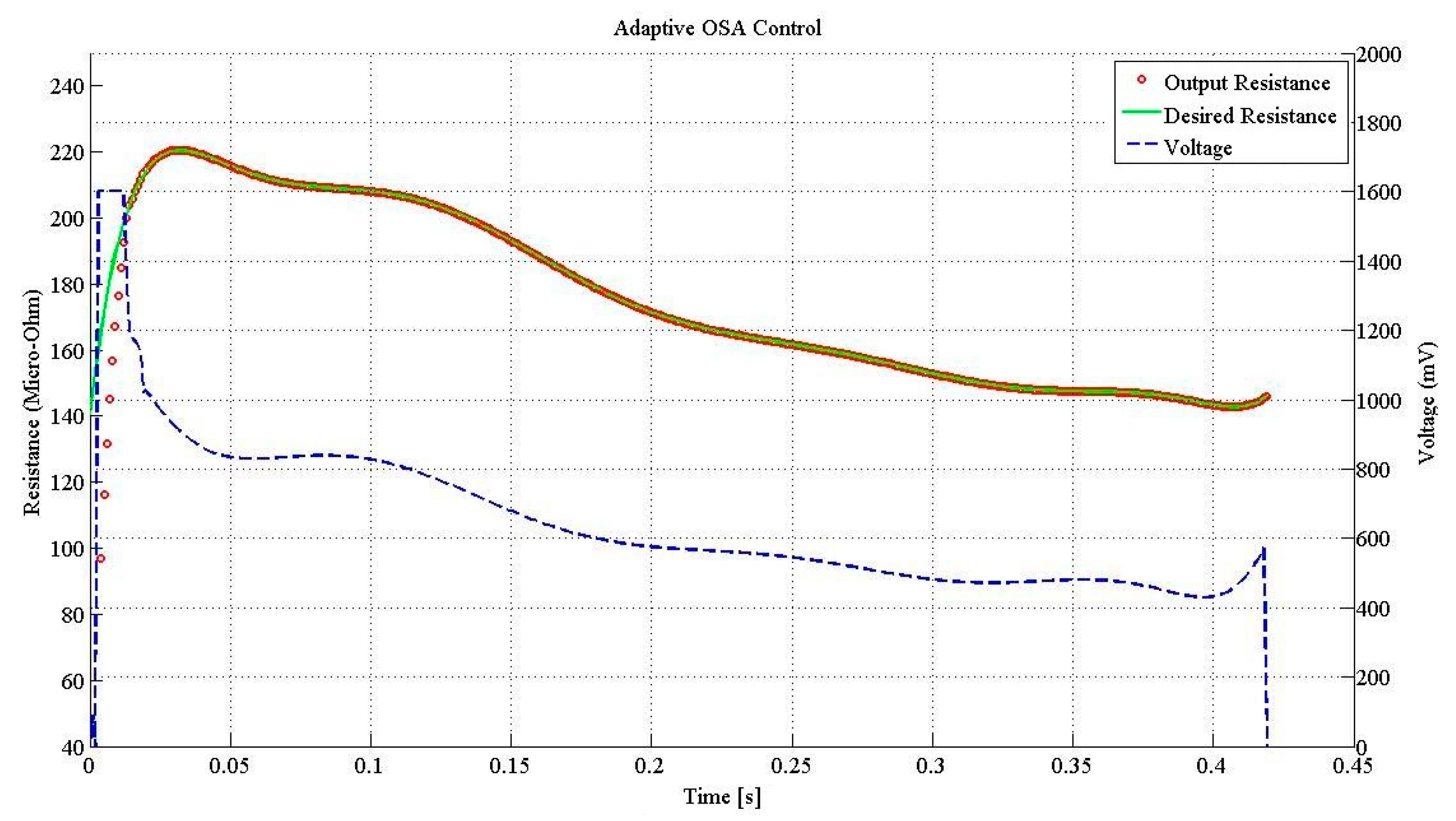
4.2. Adaptive One-Step-Ahead Tracking Controller

A one-step-ahead (OSA) RSW control scheme based on a thermal model of the RSW process was investigated in [23,24], and a similar methodology is followed here. An OSA controller attempts to bring the predicted output, $y(k+1)$ at time $k+1$, to the desired value, $y^{*}(k+1)$, in one step. Thus, it minimizes the following cost function [27]:

$$J_1(k+1)=\frac{1}{2}{[y(k+1)-y^{*}(k+1)]}^2$$

(45)

The corresponding OSA control law is given by:

$${\overline{u}}^2\left(k\right)=\frac{y^{*}\left(k+1\right)y\left(k\right)-A\left(k\right)y^2\left(k\right)-C\left(k\right)y\left(k\right)}{B\left(k\right)}$$

(46)

or equivalently,

$$\overline{u}\left(k\right)=\sqrt{\frac{y^{*}\left(k+1\right)y\left(k\right)-A\left(k\right)y^2\left(k\right)-C\left(k\right)y\left(k\right)}{B\left(k\right)}}.$$

(47)

The above control signal needs to be constrained by the maximum voltage delivery capacity of the weld controller, $u_{max}$, as follows:

$$u\left(k\right)=\{\begin{array}{cc}\overline{u}\left(k\right),& if 0<\overline{u}\left(k\right)<u_{max}\\ 0,& if \overline{u}\left(k\right)\le 0\\ u_{max},& if \overline{u}\left(k\right)\ge u_{max}\end{array}$$

(48)

The adaptive OSA controller uses the estimate, $\widehat{X}\left(k\right)$, in Equation (39) to compute the control signal, $\overline{u}\left(k\right)$, from the following adaptive version of Equation (47):

$$\overline{u}\left(k\right)=\sqrt{\frac{y^{*}\left(k+1\right)y\left(k\right)-\widehat{A}\left(k\right)y^2\left(k\right)-\widehat{C}\left(k\right)y\left(k\right)}{\widehat{B}\left(k\right)}}$$

(49)

where $\widehat{A}\left(k\right), \widehat{B}\left(k\right),$and $\widehat{C}\left(k\right)$ denote the estimated values of $A\left(k\right), B\left(k\right),$and $C\left(k\right)$, respectively, at time $k$.

Remark

Since welding times are usually very short (less than 0.5 sec), establishing proof of asymptotic tracking would be meaningless here. However, since the input voltage and output resistance are bounded in this case, the regression vector, $\phi \left(k\right)$, in Equation (36) is bounded for all k. This ensures that the RLS parameter estimation algorithm, described by Equations (39)–(42), possesses nice convergence properties [27] that help the output resistance track the reference resistance profile. Furthermore, since most RSW applications require successive welds under very similar conditions, tracking can be significantly improved by initializing the RLS parameter estimator to the nominal values of the process parameters, which essentially remain constant or change very slowly from one weld to the next.

5. Simulation Results and Discussion

The results of a simulation study to evaluate the performance of the proposed controller and compare it to that of a PID controller are presented in this section. Both controllers are designed for tracking a desired reference resistance profile.

As mentioned earlier, a reference resistance profile serves as a good indicator of the weld quality. Therefore, it is desirable to maintain the dynamic resistance of a (forming) weld nugget reasonably close to a reference resistance profile. For these simulations, two sheets of 1.2-mm-thick mild steel were used as the materials to be welded. The properties of this material and the RSW model parameters are listed in

Table 1. Material properties and RSW model parameters.

Symbol	Description	Value	Units
$\rho$	Density	7800	Kg.${\mathrm{m}}^{-3}$
$C_p$	Specific Heat	480	J.${\mathrm{Kg}}^{-1}$.${\mathrm{C}}^{-1}$
a	Nominal Nugget Radius	2.50 × 10−3	m
p	Nominal Nugget Penetration per Sheet	1.08 × 10−3	m
k	Thermal Conductivity	15.1	W.${\mathrm{m}}^{-1}$.${\mathrm{C}}^{-1}$
$l_1$	Nominal Indentation per Sheet	1.20 × 10−4	m
β	Penetration to Workpiece Thickness Ratio	0.8	no units
L	Sheet Thickness	1.20 × 10−3	m
b	Electrode Radius	3.00 × 10−3	m
$L_f$	Latent Heat of Fusion	2.73 × 105	J.${\mathrm{Kg}}^{-1}$
H	Heat of Fusion	2.13 × 109	J.${\mathrm{m}}^{-3}$
α	Thermal Diffusivity	4.03 × 10−6	${\mathrm{m}}^2$.${\mathrm{s}}^{-1}$
${\theta }_I$	Interface Temperature	500	$°\mathrm{C}$
${\theta }_{°}$	Initial Temperature	20	$°\mathrm{C}$
${\alpha }_r$	Temperature Coefficient	0.0066	$°{\mathrm{C}}^{-1}$
${\rho }_{°}$	Resistivity @ 20 $°$C	0.15	$\mathsf{\mu }\mathsf{\Omega }$.m

below.

A typical reference resistance profile for a good weld made on such a workpiece is shown in Figure 6, and it is used as a reference in this study. Depending on the error signal, the welding voltage is adjusted so as to reduce the resistance tracking error. Also, the controller is assumed to be capable of delivering a maximum voltage, V_max = 1600 mV.

Although RSW welds are usually performed under constant force, some variations of the applied pressure always occur during welding. Also, electrode tips exhibit wear and tear due to repeated hammering and deposition of metals on the tip surfaces. In view of above, force variation and electrode wear are considered to be unknown process (noise) variables that impact the nugget size (diameter and penetration). Since an RSW weld controller must be evaluated in the presence of such ubiquitous process (noise) variables, the performance of an AOSA controller and a PID controller are tested in case of a 20% increase in nugget diameter and a 50% increase in indentation from their nominal values.

Figure 7 shows the performance of the AOSA controller. It can be seen that the AOSA controller adapts to the parameter changes and enables the output resistance profile to follow the desired resistance profile reasonably well. In fact, tracking can be further improved by initializing the RLS parameter estimator to the nominal values of the process parameters. Also, the energy required to perform the weld is found to be 1180 J.

Figure 8 shows the performance of a PID controller. After a number of trials to tune the performance of the PID controller, the optimal gains of the controller were chosen to be as follows: Proportional (P) = 0.023, Integral (I) = 3.14, Derivative (D) = −6.99. At its best performance, it can be seen that the PID controller initially loses track of the reference resistance profile due to variation of welding parameters, which can be detrimental to nugget formation. Also, it can be seen that the PID controller requires more energy (1217 J) to perform the weld, as compared to AOSA.

Comparing the simulation results for the above controllers, the AOSA controller is seen to exhibit satisfactory performance and, in this case, the output resistance profile tracks the desired reference resistance profile quite well. Also, it may be noted that the total energy required to perform a weld using an AOSA controller is less compared to that used by a PID controller. In the long run, this can yield significant energy savings for applications requiring a high volume of spot welds, such as manufacturing of automotive vehicles.

6. Conclusions

This paper proposes a new theoretical approach of designing an AOSA controller for resistance spot welding that utilizes a simplified dynamic resistance model of an RSW process. The development of this model and its validation are discussed in detail. It also presents the results of a simulation study that compares the performance of the proposed AOSA controller with that of a PID controller. The simulation results indicate that an AOSA controller is capable of compensating for some process parameter variations, and also enables tracking of a desired reference resistance profile. Also, these results indicate that an AOSA controller is capable of reducing the energy consumed per weld, which may yield significant energy and cost savings for applications requiring a high volume of spot welds. It should be mentioned, however, that this paper only lays the foundation of a viable adaptive RSW control scheme based on a dynamic resistance model. Actual hardware implementation and testing of the proposed scheme is currently under investigation and results of these studies are expected to be presented in a follow-up paper.

References

1. Zhang, H.; Senkara, J. Resistance Welding Fundamentals and Applications; Taylor & Francis Group: Boca Raton, FL, USA, 2012. [Google Scholar]
2. Govik, A. Modeling of the Resistance Spot Welding Process. Master Thesis, Linköping University, Linköping, Sweden, 2009. [Google Scholar]
3. Won, Y.J.; Cho, H.S.; Lee, C.W. A Microprocessor-Based Control System for Resistance Spot Welding Process. In Proceedings of the American Control Conference, San Francisco, CA, USA, 22–24 June 1983; pp. 734–738. [Google Scholar]
4. Zhou, K.; Cai, L. A Nonlinear Current Control Method for Resistance Spot Welding. Proc. ASME Trans. Mechatron. 2014, 19, 559–569. [Google Scholar] [CrossRef]
5. Salem, M.; Brown, L.J. Improved Consistency of Resistance Spot Welding with Tip Voltage Control. In Proceedings of the 24th Canadian Conference on Electrical and Computer Engineering, Niagara Falls, ON, Canada, 8–11 May 2011; pp. 548–551. [Google Scholar]
6. Chen, X.; Araki, K.; Mizuno, T. Modeling and Fuzzy Control of the Resistance Spot Welding Process. In Proceedings of the 24th Canadian Conference on Electrical and Computer Engineering, Tokushima, Japan, 29–31 July 1997; pp. 898–994. [Google Scholar]
7. El-Banna, M.; Filev, D.; Chinnam, R.B. Intelligent Constant Current Control for Resistance Spot Welding. In Proceedings of the IEEE Conference on Fuzzy Systems, Vancouver, BC, Canada, 16–21 July 2006; pp. 1570–1577. [Google Scholar]
8. Chen, X.; Araki, K. Fuzzy Adaptive Process Control of Resistance Spot Welding with a Current Reference Model. In Proceedings of the IEEE Conference on Intelligent Processing Systems, Beijing, China, 28–31 October 1997; pp. 190–194. [Google Scholar]
9. Shriver, J.; Peng, H.; Hu, S.J. Control of Resistance Spot Welding. In Proceedings of the 1999 American Control Conference, San Diego, CA, USA, 2–4 June 1999; pp. 187–191. [Google Scholar]
10. Ivezic, N.; Allen, J.D.; Zacharia, T. Neural Network-Based Resistance Spot Welding Control and Quality Prediction. In Proceedings of the Second International Conference on Intelligent Processing and Manufacturing of Materials, Honolulu, HI, USA, 10–15 July 1999; pp. 989–994. [Google Scholar]
11. Messler, R.W.; Jou, M.; Li, C.J. An Intelligent Control System for Resistance Spot Welding Using a Neural Network and Fuzzy Logic. In Proceedings of the 1995 IEEE Industry Applications Conference Thirtieth IAS Annual Meeting, Orlando, FL, USA, 8–12 October 1995; pp. 1757–1763. [Google Scholar]
12. Yu, J. New methods of resistance spot welding using reference waveforms of welding power. Int. J. Precis. Eng. Manuf. 2016, 17, 1313–1321. [Google Scholar] [CrossRef]
13. Subbanna, R.S.; Rajini, M. Intelligent Control System for Resistance Spot Welding System. Manag. J. Instrum. Control Eng. 2018, 6, 35–41. [Google Scholar] [CrossRef]
14. Yu, J. Adaptive Resistance Spot Welding Process that Reduces the Shunting Effect for Automotive High-Strength Steels. Metals 2018, 8, 775. [Google Scholar] [CrossRef]
15. Dickinson, D.; Franklin, J.; Stanya, A. Characterization of Spot-Welding Behavior by Dynamic Electrical Parameter Monitoring. Weld. J. 1980, 59, S170–S176. [Google Scholar]
16. Kaiser, J.; Dunn, D.; Eagar, T. The Effect of Electrical-Resistance on Nugget Formation during Spot-Welding. Weld. J. 1982, 61, S167–S174. [Google Scholar]
17. Garza, F.; Das, M. On real time monitoring and control of resistance spot welds using dynamic resistance signatures. In Proceedings of the 44th IEEE 2001 Midwest Symposium on Circuits and Systems, Dayton, OH, USA, 14–17 August 2001. [Google Scholar]
18. Cho, Y.; Rhee, S. Primary Circuit Dynamic Resistance Monitoring and its Application to Quality Estimation during Resistance Spot Welding. Weld. J. 2002, 81, S104–S111. [Google Scholar]
19. Wan, X.; Wang, Y.; Zhao, D. Quality monitoring based on dynamic resistance and principal component analysis in small scale resistance spot welding process. Int. J. Adv. Manuf. Technol. 2016, 86, 3443–3451. [Google Scholar] [CrossRef]
20. Luo, Y.; Rui, W.; Xie, X.; Zhu, Y. Study on the nugget growth in single-phase AC resistance spot welding based on the calculation of dynamic resistance. J. Mater. Process. Technol. 2016, 229, 492–500. [Google Scholar] [CrossRef]
21. Podrzaj, P.; Polajnar, I.; Diaci, J.; Kariz, Z. Overview of resistance spot welding control. Sci. Technol. Weld. Join. 2008, 13, 215–224. [Google Scholar] [CrossRef]
22. Hemmati, M.; Haeri, M. Control of resistance spot welding using model predictive control. In Proceedings of the 2015 9th International Conference on Electrical and Electronics Engineering, Bursa, Turkey, 26–28 November 2015; pp. 864–868. [Google Scholar]
23. Kas, Z.; Das, M. A Thermal Dynamical Model Based Control of Resistance Spot Welding. In Proceedings of the IEEE International Conference on Electro/Information Technology, Milwaukee, WI, USA, 5–7 June 2014; pp. 264–269. [Google Scholar]
24. Kas, Z.; Das, M. An Electrothermal Model Based Adaptive Control of Resistance Spot Welding Process. Intell. Control Autom. 2015, 6, 134–146. [Google Scholar] [CrossRef] [Green Version]
25. Kim, E.W.; Eagar, T.W. Parametric Analysis of Resistance Spot Welding Lobe Curve. SAE Trans. J. Mater. 1988. [Google Scholar] [CrossRef] [Green Version]
26. CHC Algorithm, WTC. Available online: http://www.weldtechcorp.com/welding_concepts/weldsolutions_chc.html (accessed on 27 September 2019).
27. Goodwin, G.C.; Sin, K.S. Adaptive Filtering Prediction and Control; Prentice-Hall: Englewood Cliffs, NJ, USA, 1983. [Google Scholar]
Figure 1. Resistance spot welding system.
Mca 24 00086 g001
Figure 2. A simplified thermal model of nugget formation.
Mca 24 00086 g002
Figure 3. Voltage, V(t), and current, I(t), from a weld performed by a CHC controller.
Mca 24 00086 g003
Figure 4. Estimated model parameters from the voltage and current data shown in Figure 3.
Mca 24 00086 g004
Figure 5. Goodness of fit between actual dynamical resistance (shown dotted), R(t), and its model-predicted values, Rp(t).
Mca 24 00086 g005
Figure 6. Desired reference resistance profile.
Mca 24 00086 g006
Figure 7. Tracking performance of the AOSA controller. The reference resistance profile is shown as a continuous (green) curve and the actual (output) resistance is shown in (orange) circles. The control (welding) voltage, V(t), is shown as a dashed (blue) curve ( V max = 1600   mV ) . Energy consumed to perform the weld = 1180 J.
Mca 24 00086 g007
Figure 8. Tracking performance of the (tuned) PID controller. The reference resistance profile is shown as a continuous (green) curve and the actual (output) resistance is shown in (red) circles. The control (welding) voltage, V(t), is shown as a dashed (blue) curve ( V max = 1600   mV ) . Energy consumed to perform the weld = 1217 J.
Mca 24 00086 g008