Hypergraphs Based on Pythagorean Fuzzy Soft Model

Abstract

A Pythagorean fuzzy soft set (PFSS) model is an extension of an intuitionistic fuzzy soft set (IFSS) model to deal with vague knowledge according to different parameters. The PFSS model is a more powerful tool for expressing uncertain information when making decisions and it relaxes the constraint of IFSS. Hypergraphs are helpful to handle the complex relationships among objects. Here, we apply the concept of PFSSs to hypergraphs, and present the notion of Pythagorean fuzzy soft hypergraphs (PFSHs). Further, we illustrate some operations on PFSHs. Moreover, we describe the regular PFSHs, perfectly regular PFSHs and perfectly irregular PFSHs. Finally, we consider the application of PFSHs for the selection of a team of workers for business and got the appropriate result by using score function.

1. Introduction

For the modeling and solution of combinative issues that appear in different areas, including mathematics, computer science, and engineering, graph theory has become a powerful theoretical structure but only pairwise relationships are represented by graphs. In several real-world applications, relationships are more problematic among the objects, then graph theory fails to handle such relationships when we consider more than two objects. Therefore, we use hypergraphs to represent the complex relationships among the objects. In case of a set of multiarity relations, hypergraphs are the generalization of graphs, in which a hypergraph may have more than two vertices. Hypergraphs have many applications in different fields including biological science, computer science, and discrete mathematics. There are a lot of complicated problems and notions in various fields such as rewriting systems, databases and logic programming, which can be interpreted using hypergraphs presented in [1].

The notion of classical set (CS) theory is generalized by fuzzy set (FS) theory. In CS theory, information is either true or false but there is no information for the intermediate state. Many uncertain problems can be handled more accurately by using FS. Zadeh introduced the FS in 1965 to solve uncertainty problems [2]. In complex phenomena, FS theory plays an important role which is not solved by CS theory. As an extension of FS, Atanassov [3] illuminated the intuitionistic fuzzy set (IFS) by adding a non-membership function which satisfies the condition $\mu +\nu \le 1$. There are a lot of decision making problems, where the sum of membership and non-membership degrees of an object may be greater than 1 and square sum of its membership degree and non-membership degree is less than or equal to 1. To handle such difficulties, Yager [4,5] introduced the concept of Pythagorean fuzzy set (PFS) as an extension of IFS, which satisfies ${\mu }^2+{\nu }^2\le 1$ and it relaxes the constraint of IFS. Multiparametric similarity measures on Pythagorean fuzzy sets were discussed by Peng et al. [6]. Peng et al. [7] studied Pythagorean fuzzy multi-criteria decision making method based on CODAS with new score function. Fei et al. [8] worked on Pythagorean fuzzy (PF) decision making using soft likelihood functions. Fei et al. [9] studied multi-criteria decision making in PF environment. For parameterized theory of uncertainty problems, Molodstov [10] gave the idea of soft set (SS) theory. Fuzzy soft set (FSS) was defined by Maji et al. [11] and using this concept in decision making problems, Roy and Maji [12] established many applications. Peng et al. [13] studied PFSSs and its applications.

Kaufmann [14] gave the concept of fuzzy graphs (FGs) in 1973. Some operations on FGs were defined by Mordeson and Chang-Shyh [15] in 1994. Parvathi and Karunambigai [16] studied the notion of intuitionistic fuzzy graphs (IFGs). Naz et al. [17] presented the view of Pythagorean fuzzy graphs (PFGs). Some new operations of PFGs were established by Akram et al. [18]. The idea of fuzzy soft graphs (FSGs) was established by Akram and Nawaz [19]. Shahzadi and Akram [20] illustrated the concept of IFSGs. To overcome the uncertainty in crisp hypergraphs, the idea of fuzzy hypergraphs (FHs) was introduced by Kaufmann [14]. Mordeson and Nair worked on FGs as well as FHs in [21]. Chen [22] gave the notion of interval-valued FHs. Lee Kwang and Lee [23] examined the FHs with fuzzy partition. Bipolar neutrosophic hypergraphs with applications were presented by Akram and Luqman [24]. Hypergraphs in m-polar fuzzy environment are considered in [25]. Thilagavathi [26] gave the idea of intuitionistic fuzzy soft hyergraphs (IFSHs). Further new extensions of fuzzy hypergraphs are presented in [27,28]. In this paper, in Section 3, we have combined the concepts of Pythagorean fuzzy soft sets and hypergraphs, and constructed PFSHs to deal the complexity in relationships corresponding to different parameters. We have introduced the concept of strong and complete PFSHs. We have discussed certain operations on PFSHs and regularity of PFSHs. In Section 4, we have described steps of decision method. In Section 5, we have described a decision making problem to obtain a competent team for business. In Section 6, we have concluded our results related to our proposed model.

2. Preliminaries

Definition 1

([17]). A PFG on a non-empty set X is a pair $G=(A,B)$, where A is a PFS on X and B is a PFR on X such that

$${\mu }_B(x_1{x}_2)\le min\{{\mu }_A(x_1),{\mu }_A(x_2)\},{\nu }_B(x_1{x}_2)\le max\{{\nu }_A(x_1),{\nu }_A(x_2)\},$$

and ${\mu }_B^2(x_1{x}_2)+{\nu }_B^2(x_1{x}_2)\le 1$, for all $x_1,x_2\in X$.

Definition 2

([20]). An IFSG on a non-empty set X is a tuple $I_G=(\tilde{L},\tilde{K},C)$ such that

• 1. C is a non-empty set of parameters,
• 2. $(\tilde{L},C)$ is an IFSS over X,
• 3. $(\tilde{K},C)$ is an IFSS over $E\subseteq X\times X,$
• 4. $(\tilde{L}({\beta }_i),\tilde{K}({\beta }_i))$ is a connected IF subgraph for all ${\beta }_i\in C,i=1,2,\cdots ,m$. That is,

  $$\widetilde{K_{\mu }}({\beta }_i)(x_1{x}_2)\le min\{\widetilde{L_{\mu }}({\beta }_i)(x_1),\widetilde{L_{\mu }}({\beta }_i)(x_2)\},$$

  $$\widetilde{K_{\nu }}({\beta }_i)(x_1{x}_2)\le max\{\widetilde{L_{\nu }}({\beta }_i)(x_1),\widetilde{L_{\nu }}({\beta }_i)(x_2)\},$$

  such that $0\le {\tilde{K}}_{\mu }({\beta }_i)(x_1{x}_2)+{\tilde{K}}_{\nu }({\beta }_i)(x_1{x}_2)\le 1,\forall {\beta }_i\in C,x_1,x_2\in X.$
  The IF subgraph $(\tilde{L}({\beta }_i),\tilde{K}({\beta }_i))$ is denoted by $\tilde{T}({\beta }_i)=\left({\tilde{T}}_{\mu }({\beta }_i),{\tilde{T}}_{\nu }({\beta }_i)\right)$.

Throughout this paper, we will use the notations as defined in

Table 1. Notations.

Symbol	Definition
$H=(L,K,C)$	Pythagorean fuzzy soft hypergraph
${\beta }_i,i=1,2,\cdots ,m$	Parameters
$({\xi }_l,C),l=1,2,\cdots ,s$	Pythagorean fuzzy soft subsets
$(K,C)$	Pythagorean fuzzy soft relation
$T({\beta }_i)=(L({\beta }_i),K({\beta }_i)),\forall {\beta }_i\in C$	Pythagorean fuzzy subhypergraph
$O(H)$	Order of Pythagorean fuzzy soft hypergraph
$S(H)$	Size of Pythagorean fuzzy soft hypergraph

.

3. Pythagorean Fuzzy Soft Hypergraphs

Definition 3.

A Pythagorean fuzzy soft hypergraph on a non-empty set X is a 3-tuple $H=(L,K,C)$ where, $L=\{({\xi }_1,C),({\xi }_2,C),\cdots ,({\xi }_s,C)\}$ is a family of Pythagorean fuzzy soft subsets over X and $(K,C)$ is a Pythagorean fuzzy soft relation on the Pythagorean fuzzy soft subsets $({\xi }_l,C)$ such that

• 1. ${\mu }_{K({\beta }_i)}(e_l)={\mu }_{K({\beta }_i)}(\{x_1,x_2,\cdots ,x_r\})\le min\{{\mu }_{{\xi }_l({\beta }_i)}(x_1),{\mu }_{{\xi }_l({\beta }_i)}(x_2),\cdots ,{\mu }_{{\xi }_l({\beta }_i)}(x_r)\}$,
• 2. ${\nu }_{K({\beta }_i)}(e_l)={\nu }_{K({\beta }_i)}(\{x_1,x_2,\cdots ,x_r\})\le max\{{\nu }_{{\xi }_l({\beta }_i)}(x_1),{\nu }_{{\xi }_l({\beta }_i)}(x_2),\cdots ,{\nu }_{{\xi }_l({\beta }_i)}(x_r)\},$for all $x_1,x_2,\cdots ,x_r\in X.$
• 3. ${\displaystyle \bigcup _{{\beta }_i\in C}}{\displaystyle \bigcup _{1\le l\le s}}supp({\xi }_l({\beta }_i))=X,i=1,2,\cdots ,m.$
  where $(L({\beta }_i),K({\beta }_i))$ is a PF subhypergraph for all ${\beta }_i\in C.$

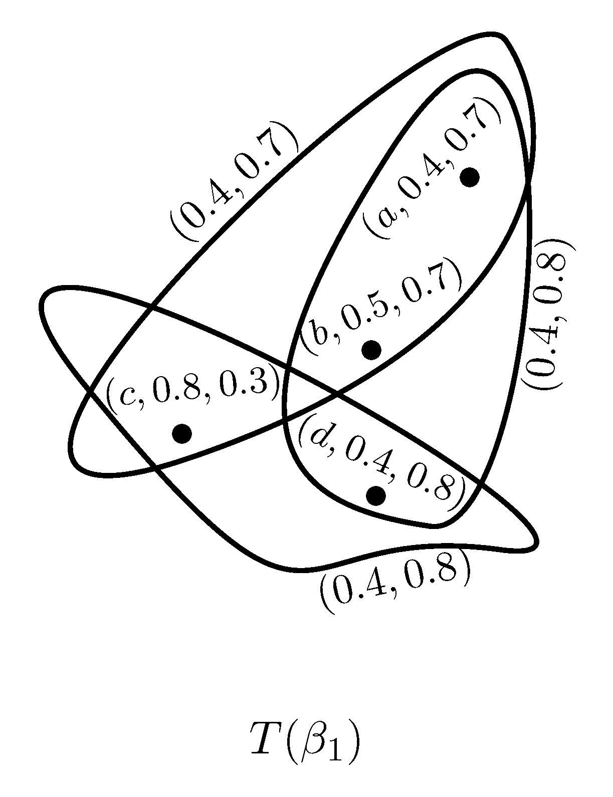
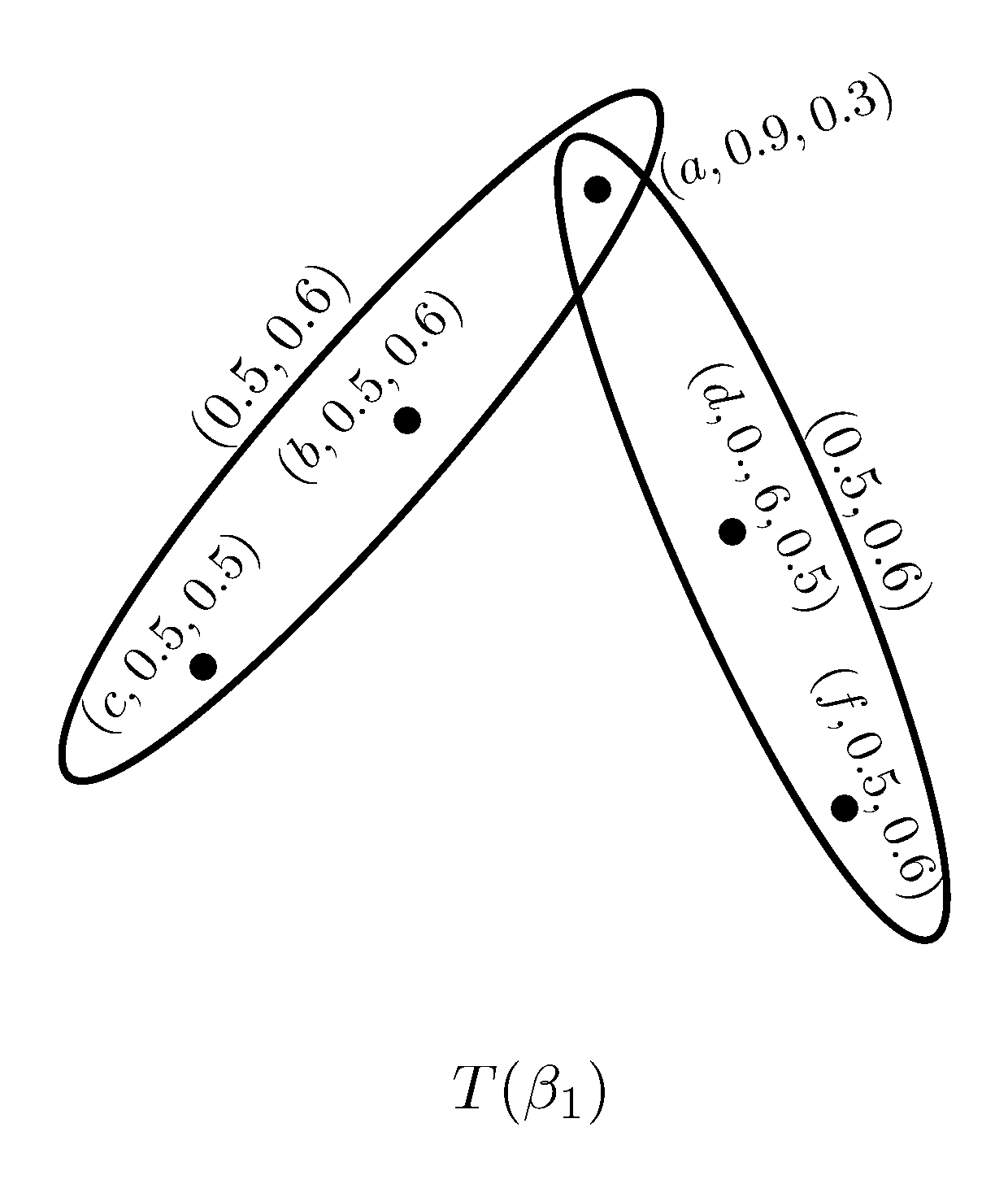
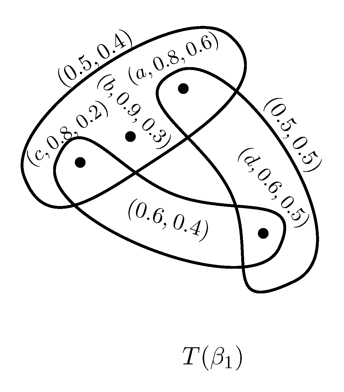
Example 1.

We present directly a PFSH $H=(L,K,C)$ on $X=\{a,b,c,d,f\}$ which is shown in Figure 1, where $C=\{{\beta }_1,{\beta }_2\}.$

Definition 4.

Let $H_1=(L_1,K_1,C_1)$ and $H_2=(L_2,K_2,C_2)$ be two PFSHs. Then $H_2$ is a PFS subhypergraph of $H_1$ if

1. 

$C_2\subseteq C_1$,

2. 

$T_2({\beta }_i)$ is a partial PF subhypergraph of $T_1({\beta }_i)$ for all ${\beta }_i\in C_2$.

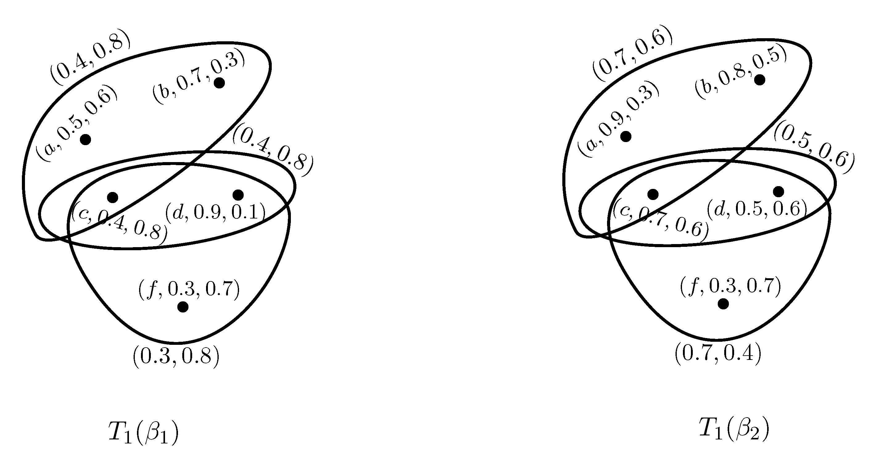
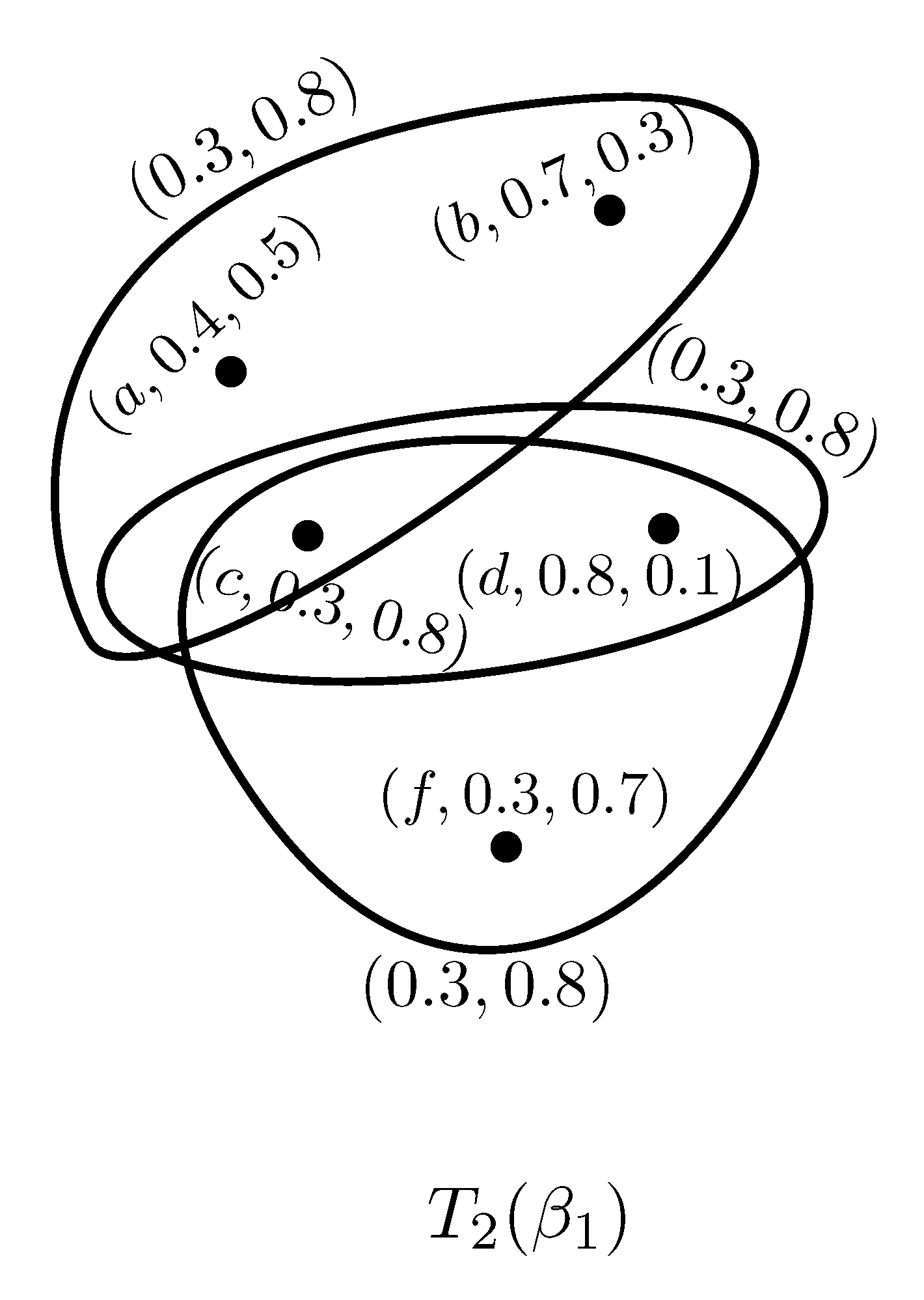
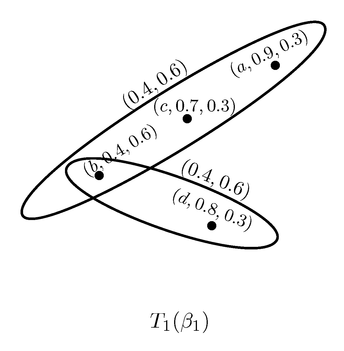
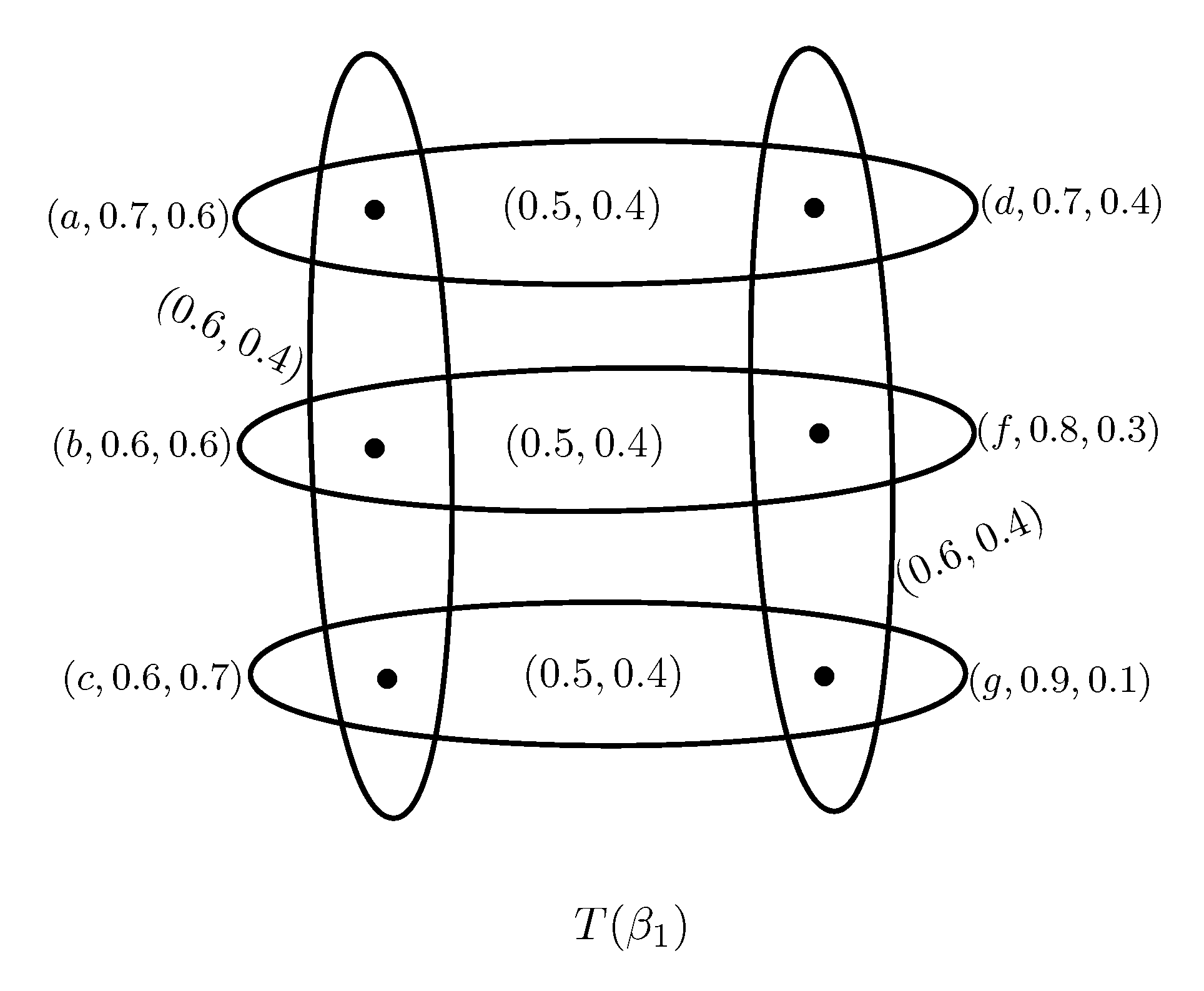
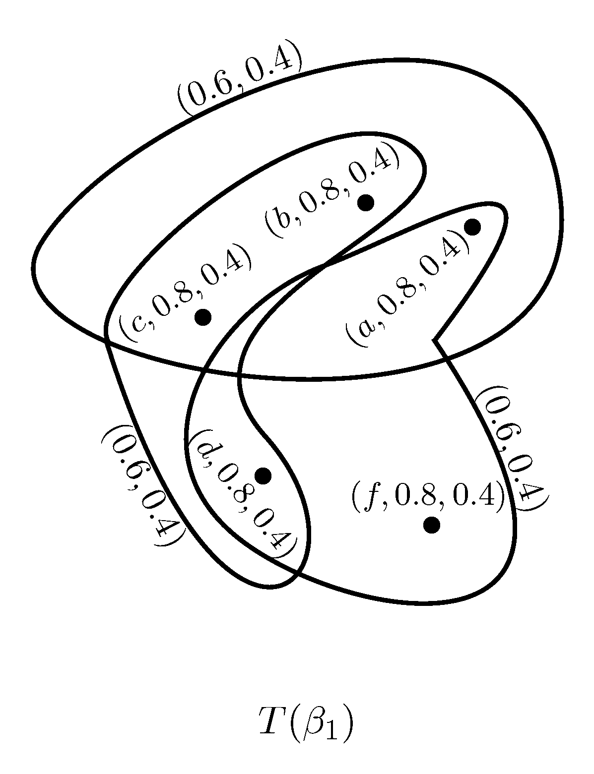
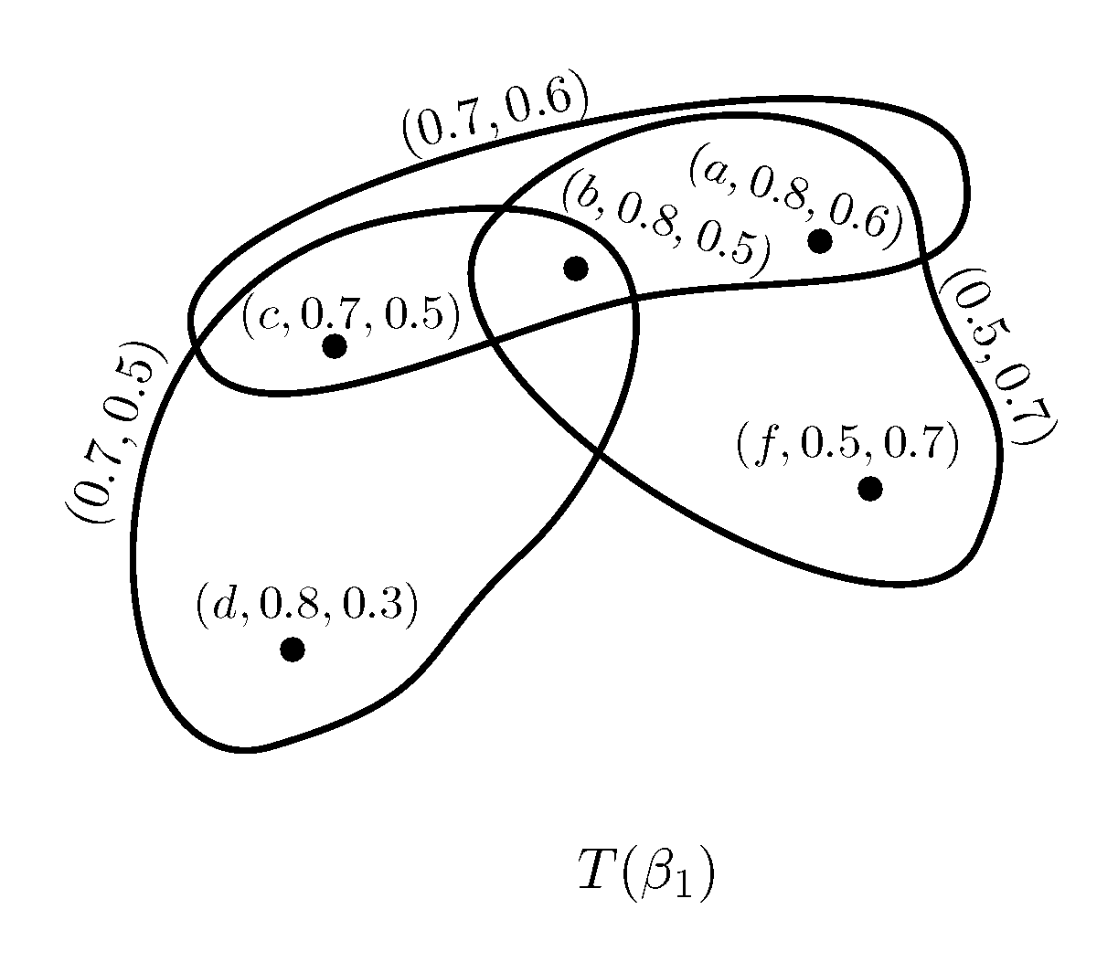
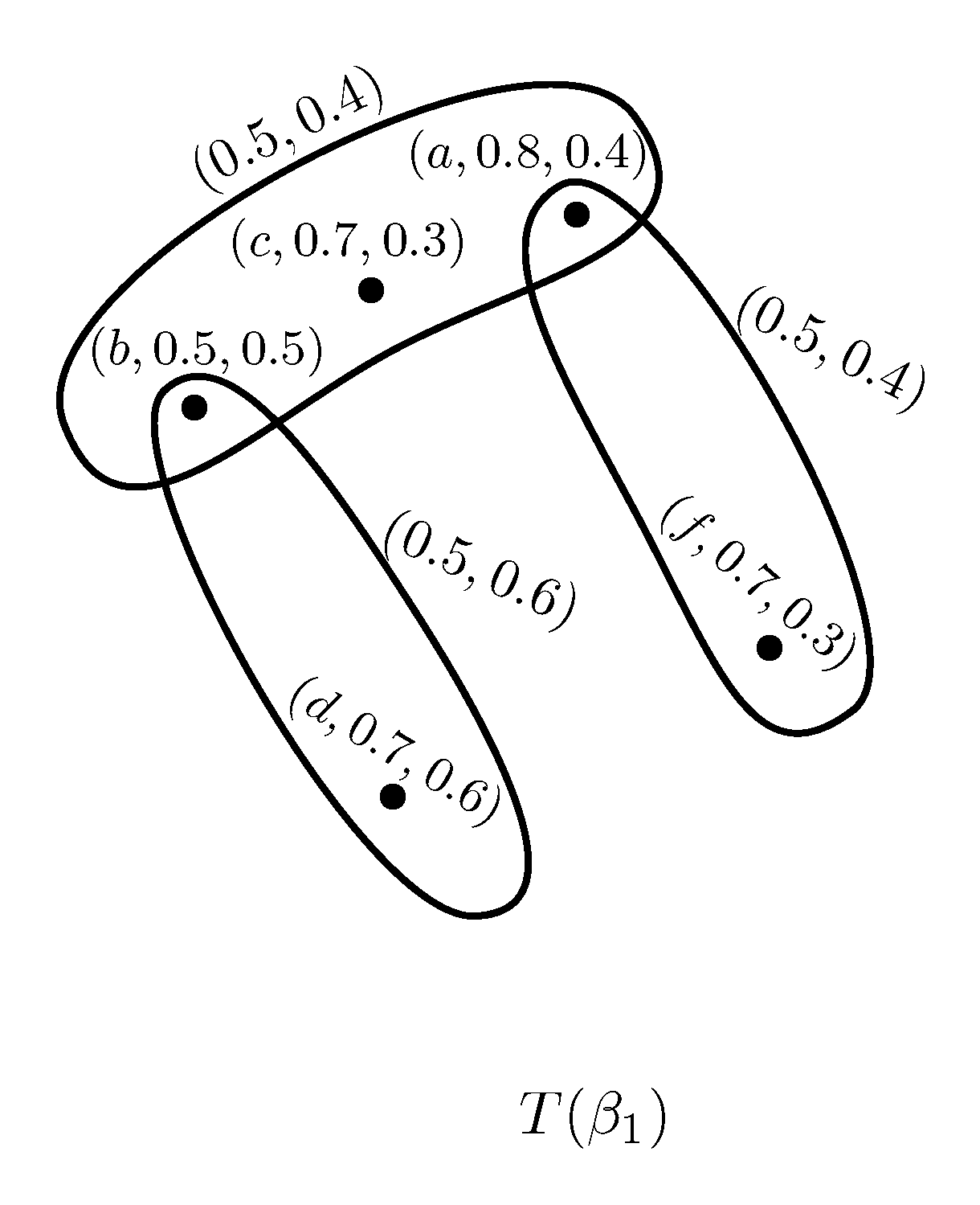
Example 2.

Consider two PFSHs $H_1$ and $H_2$ on $X=\{a,b,c,d,f\}$ as shown in Figure 2 and Figure 3, where $C_1=\{{\beta }_1,{\beta }_2\}$ and $C_2=\{{\beta }_1\}$.

Clearly, $C_2\subseteq C_1$ and $T_2({\beta }_i)$ is a partial PF subhypergraph of $T_1({\beta }_i)$ for all ${\beta }_i\in C_2$. Hence $H_2$ is a PFS subhypergraph of $H_1$.

Theorem 1.

Let $H_1=(L,K,C_1)$ and $H_2=(L,K,C_2)$ be two PFSHs. Then $H_2$ is a PFS subhypergraph of $H_1$ iff $L_2({\beta }_i)\subseteq L_1({\beta }_i)$ and $K_2({\beta }_i)\subseteq K_1({\beta }_i)$ for all ${\beta }_i\in C_2.$

Proof. 

Suppose that $H_2$ is a PFS subhypergraph of $H_1$. Then $C_2\subseteq C_1$ and $T_2({\beta }_i)$ is a partial PF subhypergraph of $T_1({\beta }_i)$ for all ${\beta }_i\in C_2$. Clearly, $L_2({\beta }_i)\subseteq L_1({\beta }_i)$ and $K_2({\beta }_i)\subseteq K_1({\beta }_i)$ for all ${\beta }_i\in C_2.$

Conversely, suppose that $L_2({\beta }_i)\subseteq L_1({\beta }_i)$ and $K_2({\beta }_i)\subseteq K_1({\beta }_i)$, for all ${\beta }_i\in C_2.$ Since $H_2$ is a PFS hypergraph, $T_2({\beta }_i)$ is a PF subhypergraph for all ${\beta }_i\in O_2$. Thus $T_2({\beta }_i)$ is a partial PF subhypergraph of $T_1({\beta }_i)$ for all ${\beta }_i\in O_2$. Hence $H_2$ is a PFS subgraph of $H_1$. □

Definition 5.

The PFSH $H_2=(L_2,K_2,C_2)$ is called spanning PFS subhypergraph of $H_1=(\widetilde{I_1},\widetilde{J_1},O_1)$ if

1. 

$C_2\subseteq C_1,$

2. 

${\mu }_{L_2({\beta }_i)}(x)={\mu }_{L_1({\beta }_i)}(x),{\nu }_{L_2({\beta }_i)}(x)={\nu }_{L_1({\beta }_i)}(x),$

for all ${\beta }_i\in C_2,x\in X$. There is no any restriction for arc weights.

Definition 6.

The order of a PFSH is

$O(H)=\left({\displaystyle \sum _{{\beta }_i\in C}}({\displaystyle \sum _{x\in X}}\wedge {\mu }_{{\xi }_l({\beta }_i)}(x)),{\displaystyle \sum _{{\beta }_i\in C}}({\displaystyle \sum _{x\in X}}\vee {\nu }_{{\xi }_l({\beta }_i)}(x))\right).$

Definition 7.

The size of a PFSH is

$S(H)=\left({\displaystyle \sum _{{\beta }_i\in C}}({\displaystyle \sum _{e_l\subset X}}{\mu }_{K({\beta }_i)}(e_l),{\displaystyle \sum _{{\beta }_i\in C}}({\displaystyle \sum _{e_l\subset X}}{\nu }_{K({\beta }_i)}(e_l))\right).$

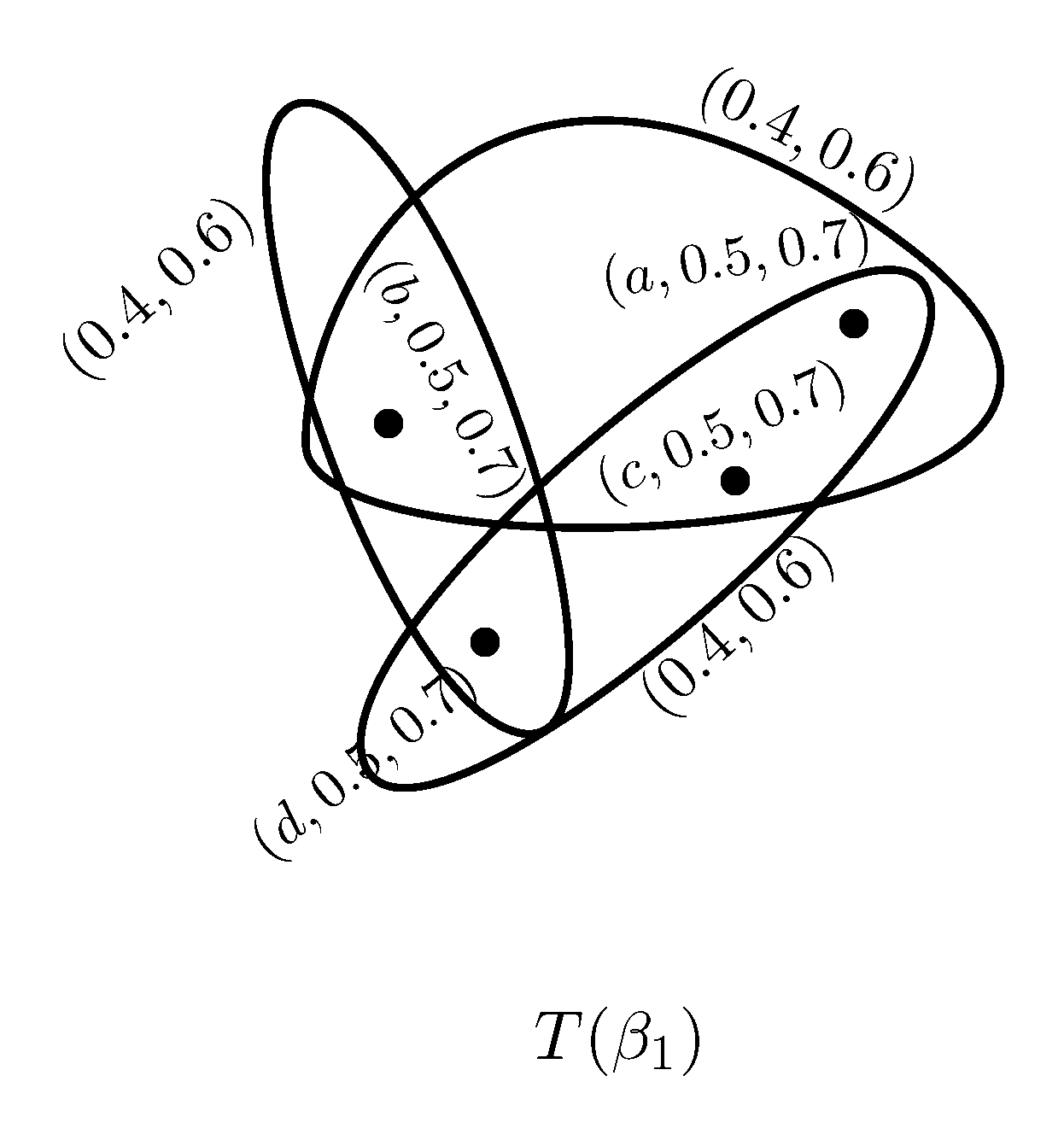
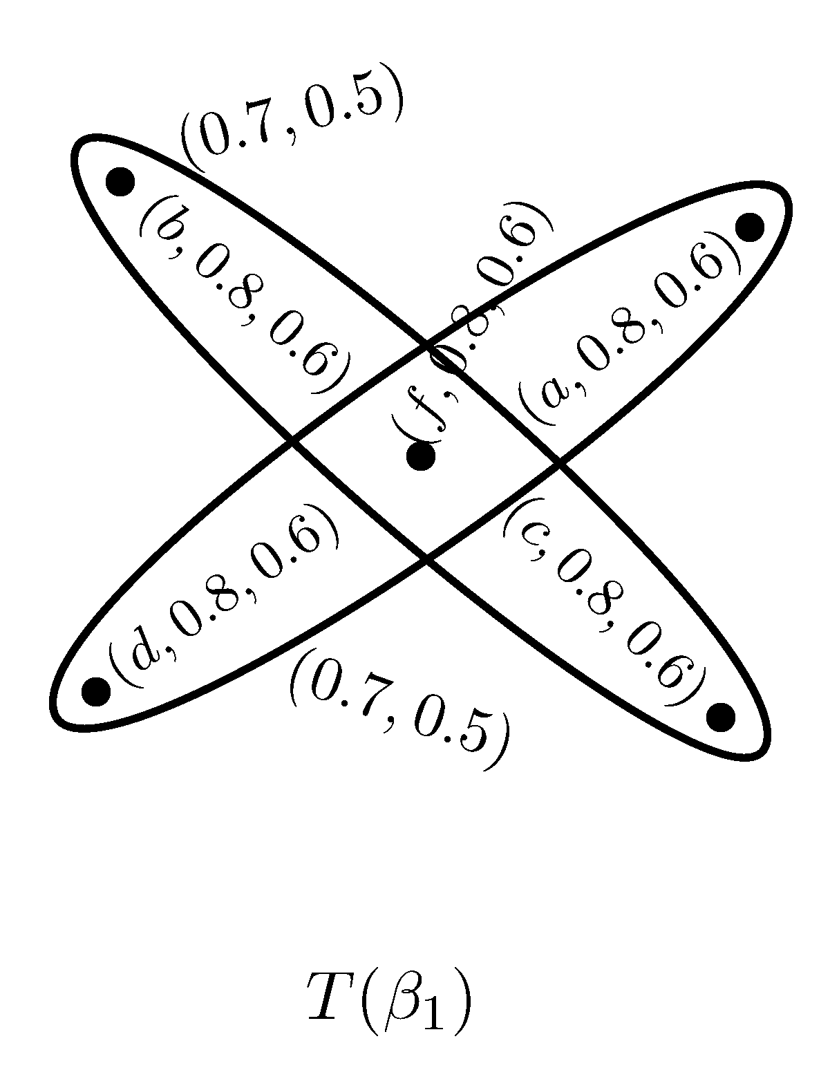
Example 3.

Consider a PFSH $H=(L,K,C)$ on $X=\{a,b,c,d\}$ as shown in Figure 4, where $C=\{{\beta }_1,{\beta }_2\}.$

Then the order of PFSH is

$$\begin{array}{ccc}O(H)& =& ((0.8+0.9+0.7+0.4)+(0.8+0.7+0.6+0.7),(0.3+0.2+0.6+0.3)\\ & & +(0.5+0.3+0.6+0.6))\\ & =& (5.6,3.4).\hfill \end{array}$$

The size of PFSH is

$$\begin{array}{ccc}S(H)& =& \left((0.4+0.7)+(0.6+0.6),(0.6+0.3)+(0.6+0.6)\right)\hfill \\ & =& (1.3,2.1).\hfill \end{array}$$

Definition 8.

A PFSH H is a strong PFSH if $T({\beta }_i)$ is a strong PFH for all ${\beta }_i\in C$. That is,

${\mu }_{K({\beta }_i)}(e_l)={\mu }_{K({\beta }_i)}(\{x_1,x_2,\cdots ,x_r\})=min\{{\mu }_{{\xi }_l({\beta }_i)}(x_1),{\mu }_{{\xi }_l({\beta }_i)}(x_2),\cdots ,{\mu }_{{\xi }_l({\beta }_i)}(x_r)\}$,

${\nu }_{K({\beta }_i)}(e_l)={\nu }_{K({\beta }_i)}(\{x_1,x_2,\cdots ,x_r\})=max\{{\mu }_{{\xi }_l({\beta }_i)}(x_1),{\mu }_{{\xi }_l({\beta }_i)}(x_2),\cdots ,{\mu }_{{\xi }_l({\beta }_i)}(x_r)\}$,

for all $e_l=\{x_1,x_2,\cdots ,x_r\}\in E.$

Example 4.

Consider a PFSH $H=(L,K,C)$ on $X=\{a,b,c,d,f\}$, where $C=\{{\beta }_1\}.$ It is cleared from Figure 5 that H is a strong PFSH.

Definition 9.

A PFSH H is a complete PFSH if $T({\beta }_i)$ is a strong PFH for all ${\beta }_i\in C$. That is,

${\mu }_{K({\beta }_i)}(e_l)={\mu }_{K({\beta }_i)}(\{x_1,x_2,\cdots ,x_r\})=min\{{\mu }_{{\xi }_l({\beta }_i)}(x_1),{\mu }_{{\xi }_l({\beta }_i)}(x_2),\cdots ,{\mu }_{{\xi }_l({\beta }_i)}(x_r)\}$,

${\nu }_{K({\beta }_i)}(e_l)={\nu }_{K({\beta }_i)}(\{x_1,x_2,\cdots ,x_r\})=max\{{\mu }_{{\xi }_l({\beta }_i)}(x_1),{\mu }_{{\xi }_l({\beta }_i)}(x_2),\cdots ,{\mu }_{{\xi }_l({\beta }_i)}(x_r)\}$,

for all $x_1,x_2,\cdots ,x_r\in X.$

Example 5.

Consider a PFSH $H=(L,K,C)$ on $X=\{a,b,c,d\}$, where $C=\{{\beta }_1\}.$ It is cleared from Figure 6 that H is a complete PFSH.

We now discuss some operations on PFSHs.

Definition 10.

Let $H_1=(L_1,K_1,C_1)$ and $H_2=(L_2,K_2,C_2)$ be two PFSHs on $X_1$ and $X_2$, respectively. Then union of $H_1$ and $H_2$, denoted by $H_1\cup H_2$, is a PFSH $(L,K,C_1\cup C_2)$, where $(L,C_1\cup C_2)=\{({\xi }_1,C_1\cup C_2),({\xi }_2,C_1\cup C_2),\cdots ,({\xi }_s,C_1\cup C_2)\}$ is a family of PFS subsets over $X=X_1\cup X_2$ and $(K,C_1\cup C_2)$ is a PFS relation on the PFS subsets $({\xi }_l,C_1\cup C_2)$ and $T({\beta }_i)=(L({\beta }_i),K({\beta }_i))$ is a PFH for all ${\beta }_i\in C_1\cup C_2$ defined by

$T({\beta }_i)=\left\{\begin{array}{c}{T}_1({\beta }_i)if{\beta }_i\in C_1-C_2,\hfill \\ T_2({\beta }_i)if{\beta }_i\in C_2-C_1,\hfill \\ T_1({\beta }_i)\cup T_2({\beta }_i)if{\beta }_i\in C_1\cap C_2,\hfill \end{array}\right.$

where $T_1({\beta }_i)\cup T_2({\beta }_i)$ denotes the union of two PFHs for all ${\beta }_i\in C_1\cap C_2$.

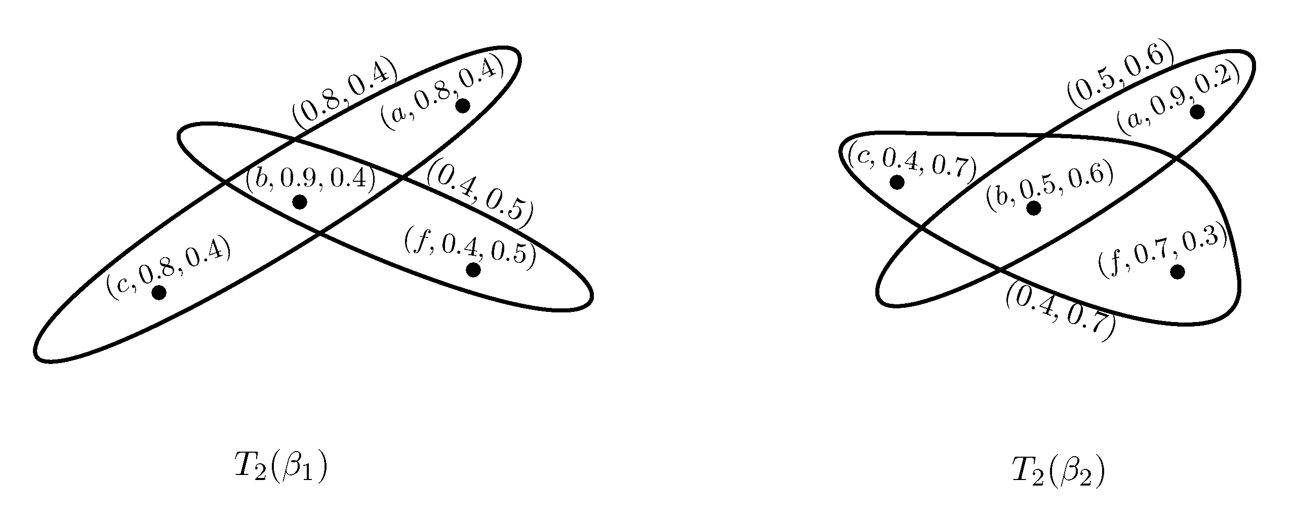
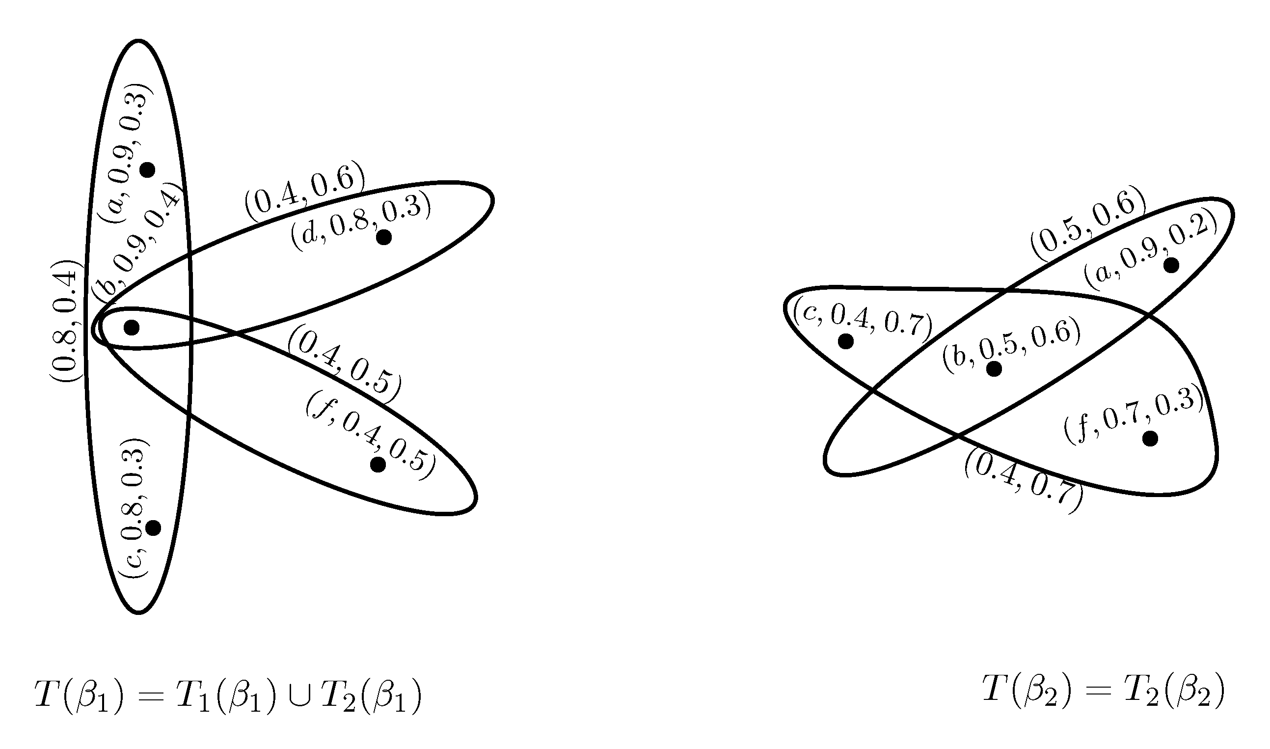
Example 6.

Consider two PFSHs $H_1=(L_1,K_1,C_1)$ and $H_2=(L_2,K_2,C_2)$ on $X_1=\{a,b,c,d\}$ and $X_2=\{a,b,c,f\}$, respectively as shown in Figure 7 and Figure 8, where $C_1=\{{\beta }_1\}$ and $C_2=\{{\beta }_1,{\beta }_2\}.$

The union of $H_1$ and $H_2$ is given in Figure 9.

Theorem 2.

Let $H_1$ and $H_2$ be two PFSHs such that $C_1\cap C_2\ne \varnothing .$ Then their union $H_1\cup H_2$ is a PFSH.

Proof. 

The union of $H_1$ and $H_2$ is defined by $H_1\cup H_2=(T,C),$ where $C=C_1\cup C_2$ and

$T({\beta }_i)=\left\{\begin{array}{c}{T}_1({\beta }_i)if{\beta }_i\in C_1-C_2,\hfill \\ T_2({\beta }_i)if{\beta }_i\in C_2-C_1,\hfill \\ T_1({\beta }_i)\cup T_2({\beta }_i)if{\beta }_i\in C_1\cap C_2.\hfill \end{array}\right.$

Since $H_1$ is a PFSH then $T_1({\beta }_i)$ is a PFH for all ${\beta }_i\in C_1$. Since $H_2$ is also a PFSH then $T_2({\beta }_i)$ is also a PFH for all ${\beta }_i\in C_2$. Since union of two PFHs is a PFH, $T_1({\beta }_i)\cup T_2({\beta }_i)$ is a PFH for all ${\beta }_i\in C_1\cap C_2$. Therefore, $T({\beta }_i)$ is a PFH for all ${\beta }_i\in C$. Thus $H_1\cup H_2=(T,C)$ is a PFSH. □

Definition 11.

Let $H_1=(L_1,K_1,C_1)$ and $H_2=(L_2,K_2,C_2)$ be two PFSHs on $X_1$ and $X_2$, respectively. Then Cartesian product of $H_1$ and $H_2$ is a PFSH $H=H_1⋉H_2=(L,K,C_1\times C_2)$, where $L_1$ and $L_2$ are Pythagorean fuzzy subsets of $X_1$ and $X_2$ and $K_1$ and $K_2$ are Pythagorean fuzzy subsets of $E_1$ and $E_2$ and $(L({\beta }_i,{\beta }_j),K({\beta }_i,{\beta }_j))$ is a PFH for all $({\beta }_i,{\beta }_j)\in C_1\times C_2$. That is,

$$\begin{array}{ccc}\hfill 1.L_{\mu }({\beta }_i,{\beta }_j)(x_1,x_2)& =& min\{{Ł}_{1\mu }({\beta }_i)(x_1),L_{2\mu }({\beta }_j)(x_2)\},\hfill \\ \hfill L_{\nu }({\beta }_i,{\beta }_j)(x_1,x_2)& =& max\{L_{1\nu }({\beta }_i)(x_1),L_{2\nu }({\beta }_j)(x_2)\},\forall (x_1,x_2)\in X,\hfill \\ \hfill 2.K_{\mu }({\beta }_i,{\beta }_j)(\{x_1\}\times e_2)& =& min\{L_{1\mu }({\beta }_i)(x_1),K_{2\mu }({\beta }_j)(e_2)\},\hfill \\ \hfill K_{\nu }({\beta }_i,{\beta }_j)(\{x_1\}\times e_2)& =& max\{L_{1\nu }({\beta }_i)(x_1),K_{2\nu }({\beta }_j)(e_2)\},\forall x_1\in X_1,e_2\in E_2,\hfill \\ \hfill 3.K_{\mu }({\beta }_i,{\beta }_j)(e_1\times \{x_2\})& =& min\{K_{1\mu }({\beta }_i)(e_1),L_{2\mu }({\beta }_j)(x_2)\},\hfill \\ \hfill K_{\nu }({\beta }_i,{\beta }_j)(e_1\times \{x_2\})& =& max\{K_{1\nu }({\beta }_i)(e_1),L_{2\nu }({\beta }_j)(x_2)\},\forall x_2\in X_2,e_1\in E_1.\hfill \end{array}$$

$T({\beta }_i,{\beta }_j)=T_1({\beta }_i)⋉T_2({\beta }_j)$ = $\{L_1({\beta }_i)⋉L_2({\beta }_j),K_1({\beta }_i)⋉K_2({\beta }_j)\},\forall ({\beta }_i,{\beta }_j)\in C_1\times C_2$, is a PFH.

Theorem 3.

The Cartesian product of two PFSHs is a PFSH.

Proof. 

Let $H_1$ and $H_2$ be two PFSHs. Let $(T,C)=\{L({\beta }_i)⋉L({\beta }_j),K({\beta }_i)⋉K({\beta }_j)\}$ be the Cartesian product of $H_1$ and $H_2$, $\forall {\beta }_i\in C_1,\forall {\beta }_j\in C_2$ for $i=1,2,\cdots ,m,j=1,2,\cdots ,n$. We claim that $(T,C)$ is a PFSH. Let $x_1\in X_1,e_1\in E_1$, suppose $e_1$ contains p vertices, where $1\le p\le n_1$ and $x_2\in X_2,e_2\in E_2$, suppose $e_2$ contains q vertices, where $1\le q\le n_2$. Then we have

Case (i): Let $x_1\in X_1,e_2\in E_2$.

$$\begin{array}{ccc}(K_{1\mu }({\beta }_i)⋉K_{2\mu }({\beta }_j))(\{x_1\}\times e_2)& =& min\{L_{1\mu }({\beta }_i)(x_1),K_{2\mu }({\beta }_j)(e_2)\}\hfill \\ & \le & min\{L_{1\mu }({\beta }_i)(x_1),{\displaystyle \underset{x_2\in e_2}{min}}{L}_{2\mu }({\beta }_j)(x_2)\}\\ & =& min\{L_{1\mu }({\beta }_i)(x_1),min\{L_{2\mu }({\beta }_j)(x_{21}),L_{2\mu }({\beta }_j)(x_{22}),\cdots ,\\ & & L_{2\mu }({\beta }_j)(x_{2q})\}\}\\ & =& min\{min\{L_{1\mu }({\beta }_i)(x_1),L_{2\mu }({\beta }_j)(x_{21})\},min\{L_{1\mu }({\beta }_i)(x_1),\\ & & L_{2\mu }({\beta }_j)(x_{22})\},\cdots ,min\{L_{1\mu }({\beta }_i)(x_1),L_{2\mu }({\beta }_j)(x_{2q})\}\}\\ & =& min\{(L_{1\mu }({\beta }_i)⋉L_{2\mu }({\beta }_j))(x_1,x_{21}),(L_{1\mu }({\beta }_i)⋉L_{2\mu }({\beta }_j))(x_1,x_{22})\\ & & ,\cdots ,(L_{1\mu }({\beta }_i)⋉L_{2\mu }({\beta }_j))(x_1,x_{2q})\}\\ & =& {\displaystyle \underset{x_1\in e_1,x_2\in e_2}{min}}(L_{1\mu }({\beta }_i)⋉L_{2\mu }({\beta }_j))(x_1,x_2),\end{array}$$

and

$$\begin{array}{ccc}(K_{1\nu }({\beta }_i)⋉K_{2\nu }({\beta }_j))(\{x_1\}\times e_2)& =& max\{L_{1\nu }({\beta }_i)(x_1),K_{2\nu }({\beta }_j)(e_2)\}\hfill \\ & \le & max\{L_{1\nu }({\beta }_i)(x_1),{\displaystyle \underset{x_2\in e_2}{max}}{L}_{2\nu }({\beta }_j)(x_2)\}\\ & =& max\{L_{1\nu }({\beta }_i)(x_1),max\{L_{2\nu }({\beta }_j)(x_{21}),L_{2\nu }({\beta }_j)(x_{22}),\cdots ,\\ & & L_{2\nu }({\beta }_j)(x_{2q})\}\}\\ & =& max\{max\{L_{1\nu }({\beta }_i)(x_1),L_{2\nu }({\beta }_j)(x_{21})\},max\{L_{1\nu }({\beta }_i)(x_1),\\ & & L_{2\nu }({\beta }_j)(x_{22})\},\cdots ,max\{L_{1\nu }({\beta }_i)(x_1),L_{2\nu }({\beta }_j)(x_{2q})\}\}\\ & =& max\{(L_{1\nu }({\beta }_i)⋉L_{2\nu }({\beta }_j))(x_1,x_{21}),(L_{1\nu }({\beta }_i)⋉L_{2\nu }({\beta }_j))(x_1,x_{22})\\ & & ,\cdots ,(L_{1\nu }({\beta }_i)⋉L_{2\nu }({\beta }_j))(x_1,x_{2q})\}\\ & =& {\displaystyle \underset{x_1\in X_1,x_2\in e_2}{max}}(L_{1\nu }({\beta }_i)⋉L_{2\nu }({\beta }_j))(x_1,x_2).\end{array}$$

Similarly, we can show that

$(K_{1\mu }({\beta }_i)⋉K_{2\mu }({\beta }_j))(e_1\times \{x_2\})\le {\displaystyle \underset{x_1\in e_1,x_2\in X_2}{min}}(L_{1\mu }({\beta }_i)⋉L_{2\mu }({\beta }_j))(x_1,x_2)$,

$(K_{1\nu }({\beta }_i)⋉K_{2\nu }({\beta }_j))(e_1\times \{x_2\})\le {\displaystyle \underset{x_1\in e_1,x_2\in X_2}{max}}(L_{1\nu }({\beta }_i)⋉L_{2\nu }({\beta }_j))(x_1,x_2).$ □

Definition 12.

Let $H_1=(L_1,K_1,C_1)$ and $H_2=(L_2,K_2,C_2)$ be two PFSHs on $X_1$ and $X_2$, respectively. Then the composition product of $H_1$ and $H_2$ is a PFSH $H=H_1\diamond H_2=(L,K,C_1\times C_2)$, where $L_1$ and $L_2$ are Pythagorean fuzzy subsets of $X_1$ and $X_2$ and $K_1$ and $K_2$ are Pythagorean fuzzy subsets of $E_1$ and $E_2$ and $(L({\beta }_i,{\beta }_j),K({\beta }_i,{\beta }_j))$ is a PFH for all $({\beta }_i,{\beta }_j)\in C_1\times C_2$. That is,

$$\begin{array}{ccc}\hfill 1.L_{\mu }({\beta }_i,{\beta }_j)(x_1,x_2)& =& min\{{Ł}_{1\mu }({\beta }_i)(x_1),L_{2\mu }({\beta }_j)(x_2)\},\hfill \\ \hfill L_{\nu }({\beta }_i,{\beta }_j)(x_1,x_2)& =& max\{L_{1\nu }({\beta }_i)(x_1),L_{2\nu }({\beta }_j)(x_2)\},\forall (x_1,x_2)\in X,\hfill \\ \hfill 2.K_{\mu }({\beta }_i,{\beta }_j)(\{x_1\}\times e_2)& =& min\{L_{1\mu }({\beta }_i)(x_1),K_{2\mu }({\beta }_j)(e_2)\},\hfill \\ \hfill K_{\nu }({\beta }_i,{\beta }_j)(\{x_1\}\times e_2)& =& max\{L_{1\nu }({\beta }_i)(x_1),K_{2\nu }({\beta }_j)(e_2)\},\forall x_1\in X_1,e_2\in E_2,\hfill \\ \hfill 3.K_{\mu }({\beta }_i,{\beta }_j)(e_1\times \{x_2\})& =& min\{K_{1\mu }({\beta }_i)(e_1),L_{2\mu }({\beta }_j)(x_2)\},\hfill \\ \hfill K_{\nu }({\beta }_i,{\beta }_j)(e_1\times \{x_2\})& =& max\{K_{1\nu }({\beta }_i)(e_1),L_{2\nu }({\beta }_j)(x_2)\},\forall x_2\in X_2,e_1\in E_1,\hfill \\ \hfill 4.K_{\mu }({\beta }_i,{\beta }_j)((x_{11},x_{21})(x_{12},x_{22})\cdots (x_{1p},x_{2q}))& =& min\{K_{1\mu }({\beta }_i)(e_1),L_{2\mu }({\beta }_j)(x_{21}),L_{2\mu }({\beta }_j)(x_{22}),\cdots ,\hfill \\ & & L_{2\mu }({\beta }_j)(x_{2q})\}\hfill \\ \hfill K_{\nu }({\beta }_i,{\beta }_j)((x_{11},x_{21})(x_{12},x_{22})\cdots (x_{1p},x_{2q}))& =& max\{K_{1\nu }({\beta }_i)(e_1),L_{2\nu }({\beta }_j)(x_{21}),L_{2\nu }({\beta }_j)(x_{22}),\cdots ,\hfill \\ & & L_{2\nu }({\beta }_j)(x_{2q})\}\hfill \end{array}$$

$T({\beta }_i,{\beta }_j)=T_1({\beta }_i)\diamond T_2({\beta }_j)$ = $\{L_1({\beta }_i)\diamond L_2({\beta }_j),K_1({\beta }_i)\diamond K_2({\beta }_j)\},\forall ({\beta }_i,{\beta }_j)\in C_1\times C_2$, is a PFH.

Theorem 4.

The composition product of two PFSHs is a PFSH.

Proof. 

Case (i): Let $x_1\in X_1,e_2\in E_2$.

$$\begin{array}{ccc}(K_{1\mu }({\beta }_i)\diamond K_{2\mu }({\beta }_j))(\{x_1\}\times e_2)& =& min\{L_{1\mu }({\beta }_i)(x_1),K_{2\mu }({\beta }_j)(e_2)\}\hfill \\ & \le & min\{L_{1\mu }({\beta }_i)(x_1),{\displaystyle \underset{x_2\in e_2}{min}}{L}_{2\mu }({\beta }_j)(x_2)\}\hfill \\ & =& min\{L_{1\mu }({\beta }_i)(x_1),min\{L_{2\mu }({\beta }_j)(x_{21}),L_{2\mu }({\beta }_j)(x_{22}),\cdots ,\hfill \\ & & L_{2\mu }({\beta }_j)(x_{2q})\}\}\hfill \\ & =& min\{min\{L_{1\mu }({\beta }_i)(x_1),L_{2\mu }({\beta }_j)(x_{21})\},min\{L_{1\mu }({\beta }_i)(x_1),\hfill \\ & & L_{2\mu }({\beta }_j)(x_{22})\},\cdots ,min\{L_{1\mu }({\beta }_i)(x_1),L_{2\mu }({\beta }_j)(x_{2q})\}\}\hfill \\ & =& min\{(L_{1\mu }({\beta }_i)\diamond L_{2\mu }({\beta }_j))(x_1,x_{21}),(L_{1\mu }({\beta }_i)\diamond L_{2\mu }({\beta }_j))(x_1,x_{22})\hfill \\ & & ,\cdots ,(L_{1\mu }({\beta }_i)\diamond L_{2\mu }({\beta }_j))(x_1,x_{2q})\}\hfill \\ & =& {\displaystyle \underset{x_1\in e_1,x_2\in e_2}{min}}(L_{1\mu }({\beta }_i)\diamond L_{2\mu }({\beta }_j))(x_1,x_2),\hfill \end{array}$$

and

$$\begin{array}{ccc}(K_{1\nu }({\beta }_i)\diamond K_{2\nu }({\beta }_j))(\{x_1\}\times e_2)& =& max\{L_{1\nu }({\beta }_i)(x_1),K_{2\nu }({\beta }_j)(e_2)\}\hfill \\ & \le & max\{L_{1\nu }({\beta }_i)(x_1),{\displaystyle \underset{x_2\in e_2}{max}}{L}_{2\nu }({\beta }_j)(x_2)\}\hfill \\ & =& max\{L_{1\nu }({\beta }_i)(x_1),max\{L_{2\nu }({\beta }_j)(x_{21}),L_{2\nu }({\beta }_j)(x_{22}),\cdots ,\hfill \\ & & L_{2\nu }({\beta }_j)(x_{2q})\}\}\hfill \\ & =& max\{max\{L_{1\nu }({\beta }_i)(x_1),L_{2\nu }({\beta }_j)(x_{21})\},max\{L_{1\nu }({\beta }_i)(x_1),\hfill \\ & & L_{2\nu }({\beta }_j)(x_{22})\},\cdots ,max\{L_{1\nu }({\beta }_i)(x_1),L_{2\nu }({\beta }_j)(x_{2q})\}\}\hfill \\ & =& max\{(L_{1\nu }({\beta }_i)\diamond L_{2\nu }({\beta }_j))(x_1,x_{21}),(L_{1\nu }({\beta }_i)\diamond L_{2\nu }({\beta }_j))(x_1,x_{22})\hfill \\ & & ,\cdots ,(L_{1\nu }({\beta }_i)\diamond L_{2\nu }({\beta }_j))(x_1,x_{2q})\}\hfill \\ & =& {\displaystyle \underset{x_1\in X_1,x_2\in e_2}{max}}(L_{1\nu }({\beta }_i)\diamond L_{2\nu }({\beta }_j))(x_1,x_2).\hfill \end{array}$$

Similarly, we can show that for case (ii)

$(K_{1\mu }({\beta }_i)\diamond K_{2\mu }({\beta }_j))(e_1\times \{x_2\})\le {\displaystyle \underset{x_1\in e_1,x_2\in X_2}{min}}(L_{1\mu }({\beta }_i)\diamond L_{2\mu }({\beta }_j))(x_1,x_2)$,

$(K_{1\nu }({\beta }_i)\diamond K_{2\nu }({\beta }_j))(e_1\times \{x_2\})\le {\displaystyle \underset{x_1\in e_1,x_2\in X_2}{max}}(L_{1\nu }({\beta }_i)\diamond L_{2\nu }({\beta }_j))(x_1,x_2).$

Case (iii): Let $e_1\in E_1,x_{21},x_{22},\cdots ,x_{2q}\in X_2$.

$$\begin{array}{ccc}(K_{1\mu }({\beta }_i)\diamond K_{2\mu }({\beta }_j))((x_{11},x_{21})(x_{12},x_{22})\cdots (x_{1p},x_{2q}))& =& min\{K_{1\mu }({\beta }_i)(e_1),L_{2\mu }({\beta }_j)(x_{21}),L_{2\mu }({\beta }_j)(x_{22}),\hfill \\ & & \cdots ,L_{2\mu }({\beta }_j)(x_{2q})\}\\ & \le & min\{{\displaystyle \underset{x_1\in e_1}{min}}{L}_{1\mu }(x_1),L_{2\mu }(x_{21}),L_{2\mu }(x_{22}),\hfill \\ & & \cdots ,L_{2\mu }(x_{2q})\}\hfill \\ & =& min\{min\{L_{1\mu }(x_{11}),L_{1\mu }(x_{12}),\cdots ,L_{1\mu }(x_{1p})\},\hfill \\ & & L_{2\mu }(x_{21}),L_{2\mu }(x_{22}),\cdots ,L_{2\mu }(x_{2q})\}\hfill \\ & =& min\{min\{L_{1\mu }(x_{11}),L_{2\mu }(x_{21})\},min\{L_{1\mu }(x_{12}),\hfill \\ & & L_{2\mu }(x_{22})\},\cdots ,min\{L_{1\mu }(x_{1p}),L_{2\mu }(x_{2q})\}\}\hfill \\ & =& min\{(L_{1\mu }\diamond L_{2\mu })(x_{11},x_{21}),(L_{1\mu }\diamond L_{2\mu })(x_{12},x_{22}),\hfill \\ & & \cdots ,(L_{1\mu }\diamond L_{2\mu })(x_{1p},x_{2q})\}\hfill \\ & =& {\displaystyle \underset{x_1\in e_1,x_2\in e_2}{min}}(L_{1\mu }\diamond L_{2\mu })(x_1,x_2),\hfill \end{array}$$

and

$$\begin{array}{ccc}(K_{1\nu }({\beta }_i)\diamond K_{2\nu }({\beta }_j))((x_{11},x_{21})(x_{12},x_{22})\cdots (x_{1p},x_{2q}))& =& max\{K_{1\nu }({\beta }_i)(e_1),L_{2\nu }({\beta }_j)(x_{21}),L_{2\nu }({\beta }_j)(x_{22}),\hfill \\ & & \cdots ,L_{2\nu }({\beta }_j)(x_{2q})\}\hfill \\ & \le & max\{{\displaystyle \underset{x_1\in e_1}{max}}{L}_{1\nu }(x_1),L_{2\nu }(x_{21}),L_{2\nu }(x_{22}),\cdots ,\hfill \\ & & L_{2\nu }(x_{2q})\}\hfill \\ & =& max\{max\{L_{1\nu }(x_{11}),L_{1\nu }(x_{12}),\cdots ,L_{1\nu }(x_{1p})\},\hfill \\ & & L_{2\nu }(x_{21}),L_{2\nu }(x_{22}),\cdots ,L_{2\nu }(x_{2q})\}\hfill \\ & =& max\{max\{L_{1\nu }(x_{11}),L_{2\nu }(x_{21})\},max\{L_{1\nu }(x_{12}),\hfill \\ & & L_{2\nu }(x_{22})\},\cdots ,max\{L_{1\nu }(x_{1p}),L_{2\nu }(x_{2q})\}\}\hfill \\ & =& max\{(L_{1\nu }\diamond L_{2\nu })(x_{11},x_{21}),(L_{1\nu }\diamond L_{2\nu })(x_{12},x_{22}),\hfill \\ & & \cdots ,(L_{1\nu }\diamond L_{2\nu })(x_{1p},x_{2q})\}\hfill \\ & =& {\displaystyle \underset{x_1\in e_1,x_2\in e_2}{max}}(L_{1\nu }\diamond L_{2\nu })(x_1,x_2).\hfill \end{array}$$

 □

Now we define the concept of a PFS uniform hypergraph and strong and lexicographic products of PFS uniform hypergraphs.

Definition 13.

A PFSH H is called a PFS uniform hypergraph if $T({\beta }_i)$ is a PF $(d_i,d_i^{\prime })$-uniform hypergraph, i.e, for all $|supp({\mu }_{K({\beta }_i)},{\nu }_{K({\beta }_i)})|=(d_i,d_i^{\prime })$, $\forall {\beta }_i\in C$.

Example 7.

Consider a PFSH H on $X=\{a,b,c,d,f\},$ where $C=\{{\beta }_1\}$. It is cleared from Figure 10 that H is a PFS uniform hypergraph.

Definition 14.

Let $H_1=(L_1,K_1,C_1)$ and $H_2=(L_2,K_2,C_2)$ be two PFS uniform hypergraphs on $X_1$ and $X_2$, respectively. Then strong product of $H_1$ and $H_2$ is a PFS uniform hypergraph $H=H_1\overline{⊠}{H}_2=(L,K,C_1\times C_2)$, where $L_1$ and $L_2$ are Pythagorean fuzzy subsets of $X_1$ and $X_2$ and $K_1$ and $K_2$ are Pythagorean fuzzy subsets of $E_1$ and $E_2$ and $(L({\beta }_i,{\beta }_j),K({\beta }_i,{\beta }_j))$ is a PFH for all $({\beta }_i,{\beta }_j)\in C_1\times C_2$. That is,

$$\begin{array}{ccc}\hfill 1.L_{\mu }({\beta }_i,{\beta }_j)(x_1,x_2)& =& min\{{Ł}_{1\mu }({\beta }_i)(x_1),L_{2\mu }({\beta }_j)(x_2)\},\hfill \\ \hfill L_{\nu }({\beta }_i,{\beta }_j)(x_1,x_2)& =& max\{L_{1\nu }({\beta }_i)(x_1),L_{2\nu }({\beta }_j)(x_2)\},\forall (x_1,x_2)\in X,\hfill \\ \hfill 2.K_{\mu }({\beta }_i,{\beta }_j)(\{x_1\}\times e_2)& =& min\{L_{1\mu }({\beta }_i)(x_1),K_{2\mu }({\beta }_j)(e_2)\},\hfill \\ \hfill K_{\nu }({\beta }_i,{\beta }_j)(\{x_1\}\times e_2)& =& max\{L_{1\nu }({\beta }_i)(x_1),K_{2\nu }({\beta }_j)(e_2)\},\forall x_1\in X_1,e_2\in E_2,\hfill \\ \hfill 3.K_{\mu }({\beta }_i,{\beta }_j)(e_1\times \{x_2\})& =& min\{K_{1\mu }({\beta }_i)(e_1),L_{2\mu }({\beta }_j)(x_2)\},\hfill \\ \hfill K_{\nu }({\beta }_i,{\beta }_j)(e_1\times \{x_2\})& =& max\{K_{1\nu }({\beta }_i)(e_1),L_{2\nu }({\beta }_j)(x_2)\},\forall x_2\in X_2,e_1\in E_1,\hfill \\ \hfill 4.K_{\mu }({\beta }_i,{\beta }_j)(e_1\times e_2)& =& min\{K_{1\mu }(e_1),K_{2\mu }(e_2)\}\hfill \\ \hfill K_{\nu }({\beta }_i,{\beta }_j)(e_1\times e_2)& =& max\{K_{1\nu }(e_1),K_{2\nu }(e_2)\},\forall e_1\in E_1,\forall e_2\in E_2.\hfill \end{array}$$

$T({\beta }_i,{\beta }_j)=T_1({\beta }_i)\overline{⊠}{T}_2({\beta }_j)$ = $\{L_1({\beta }_i)\overline{⊠}{L}_2({\beta }_j),K_1({\beta }_i)\overline{⊠}{K}_2({\beta }_j)\},\forall ({\beta }_i,{\beta }_j)\in C_1\times C_2$, is a PFH.

Theorem 5.

If $H_1$ and $H_2$ are the PFS uniform hypergraphs, then $H_1\overline{⊠}{H}_2$ is a PFS uniform hypergraph.

Proof. 

Case (i): Let $x_1\in X_1,e_2\in E_2$.

$$\begin{array}{ccc}(K_{1\mu }({\beta }_i)\overline{⊠}{K}_{2\mu }({\beta }_j))(\{x_1\}\times e_2)& =& min\{L_{1\mu }({\beta }_i)(x_1),K_{2\mu }({\beta }_j)(e_2)\}\hfill \\ & \le & min\{L_{1\mu }({\beta }_i)(x_1),{\displaystyle \underset{x_2\in e_2}{min}}{L}_{2\mu }({\beta }_j)(x_2)\}\hfill \\ & =& min\{L_{1\mu }({\beta }_i)(x_1),min\{L_{2\mu }({\beta }_j)(x_{21}),L_{2\mu }({\beta }_j)(x_{22}),\cdots ,\hfill \\ & & L_{2\mu }({\beta }_j)(x_{2q})\}\}\hfill \\ & =& min\{min\{L_{1\mu }({\beta }_i)(x_1),L_{2\mu }({\beta }_j)(x_{21})\},min\{L_{1\mu }({\beta }_i)(x_1),\hfill \\ & & L_{2\mu }({\beta }_j)(x_{22})\},\cdots ,min\{L_{1\mu }({\beta }_i)(x_1),L_{2\mu }({\beta }_j)(x_{2q})\}\}\hfill \\ & =& min\{(L_{1\mu }({\beta }_i)\overline{⊠}{L}_{2\mu }({\beta }_j))(x_1,x_{21}),(L_{1\mu }({\beta }_i)\overline{⊠}{L}_{2\mu }({\beta }_j))(x_1,x_{22}),\cdots \hfill \\ & & ,(L_{1\mu }({\beta }_i)\overline{⊠}{L}_{2\mu }({\beta }_j))(x_1,x_{2q})\}\hfill \\ & =& {\displaystyle \underset{x_1\in e_1,x_2\in e_2}{min}}(L_{1\mu }({\beta }_i)\overline{⊠}{L}_{2\mu }({\beta }_j))(x_1,x_2),\hfill \end{array}$$

and

$$\begin{array}{ccc}(K_{1\nu }({\beta }_i)\overline{⊠}{K}_{2\nu }({\beta }_j))(\{x_1\}\times e_2)& =& max\{L_{1\nu }({\beta }_i)(x_1),K_{2\nu }({\beta }_j)(e_2)\}\hfill \\ & \le & max\{L_{1\nu }({\beta }_i)(x_1),{\displaystyle \underset{x_2\in e_2}{max}}{L}_{2\nu }({\beta }_j)(x_2)\}\hfill \\ & =& max\{L_{1\nu }({\beta }_i)(x_1),max\{L_{2\nu }({\beta }_j)(x_{21}),L_{2\nu }({\beta }_j)(x_{22}),\cdots ,\hfill \\ & & L_{2\nu }({\beta }_j)(x_{2q})\}\}\hfill \\ & =& max\{max\{L_{1\nu }({\beta }_i)(x_1),L_{2\nu }({\beta }_j)(x_{21})\},max\{L_{1\nu }({\beta }_i)(x_1),\hfill \\ & & L_{2\nu }({\beta }_j)(x_{22})\},\cdots ,max\{L_{1\nu }({\beta }_i)(x_1),L_{2\nu }({\beta }_j)(x_{2q})\}\}\hfill \\ & =& max\{(L_{1\nu }({\beta }_i)\overline{⊠}{L}_{2\nu }({\beta }_j))(x_1,x_{21}),(L_{1\nu }({\beta }_i)\overline{⊠}{L}_{2\nu }({\beta }_j))(x_1,x_{22}),\cdots \hfill \\ & & ,(L_{1\nu }({\beta }_i)\overline{⊠}{L}_{2\nu }({\beta }_j))(x_1,x_{2q})\}\hfill \\ & =& {\displaystyle \underset{x_1\in X_1,x_2\in e_2}{max}}(L_{1\nu }({\beta }_i)\overline{⊠}{L}_{2\nu }({\beta }_j))(x_1,x_2).\hfill \end{array}$$

Similarly, we can show that for case (ii)

$(K_{1\mu }({\beta }_i)\overline{⊠}{K}_{2\mu }({\beta }_j))(e_1\times \{x_2\})\le {\displaystyle \underset{x_1\in e_1,x_2\in X_2}{min}}(L_{1\mu }({\beta }_i)\overline{⊠}{L}_{2\mu }({\beta }_j))(x_1,x_2)$,

$(K_{1\nu }({\beta }_i)\overline{⊠}{K}_{2\nu }({\beta }_j))(e_1\times \{x_2\})\le {\displaystyle \underset{x_1\in e_1,x_2\in X_2}{max}}(L_{1\nu }({\beta }_i)\overline{⊠}{L}_{2\nu }({\beta }_j))(x_1,x_2).$

Case (iii): Let $e_1\in E_1,e_2\in E_2$.

$$\begin{array}{ccc}(K_{1\mu }({\beta }_i)\overline{⊠}{K}_{2\mu }({\beta }_j))(e_1\times e_2)& =& min\{K_{1\mu }(e_1),K_{2\mu }(e_2)\}\hfill \\ & \le & min\{{\displaystyle \underset{x_1\in e_1}{min}}{L}_{1\mu }(x_1),{\displaystyle \underset{x_2\in e_2}{min}}{L}_{2\mu }(x_2)\}\hfill \\ & =& min\{min\{L_{1\mu }(x_{11}),L_{1\mu }(x_{12}),\cdots ,L_{1\mu }(x_{1r})\},\hfill \\ & & min\{L_{2\mu }(x_{21}),L_{2\mu }(x_{22}),\cdots ,L_{2\mu }(x_{2r})\}\}\hfill \\ & =& min\{min\{L_{1\mu }(x_{11}),L_{2\mu }(x_{21})\},min\{L_{1\mu }(x_{12}),L_{2\mu }(x_{22})\}\hfill \\ & & ,\cdots ,min\{L_{1\mu }(x_{1r}),L_{\mu }2(x_{2r})\}\}\hfill \\ & =& min\{(L_{1\mu }\overline{⊠}{L}_{2\mu })(x_{11},x_{21}),(L_{1\mu }\overline{⊠}{L}_{2\mu })(x_{12},x_{22}),\cdots ,\hfill \\ & & (L_{1\mu }\overline{⊠}{L}_{2\mu })(x_{1r},x_{2r})\}\hfill \\ & =& {\displaystyle \underset{x_1\in e_1,x_2\in e_2}{min}}(L_{1\mu }\overline{⊠}{L}_{2\mu })(x_1,x_2),\hfill \end{array}$$

and

$$\begin{array}{ccc}(K_{1\nu }({\beta }_i)\overline{⊠}{K}_{2\nu }({\beta }_j))(e_1\times e_2)& =& max\{K_{1\nu }(e_1),K_{2\nu }(e_2)\}\hfill \\ & \le & max\{{\displaystyle \underset{x_1\in e_1}{max}}{L}_{1\nu }(x_1),{\displaystyle \underset{x_2\in e_2}{max}}{L}_{2\nu }(x_2)\}\hfill \\ & =& max\{max\{L_{1\nu }(x_{11}),L_{1\nu }(x_{12}),\cdots ,L_{1\nu }(x_{1r})\},\hfill \\ & & max\{L_{2\nu }(x_{21}),L_{2\nu }(x_{22}),\cdots ,L_{2\nu }(x_{2r})\}\}\hfill \\ & =& max\{max\{L_{1\nu }(x_{11}),L_{2\nu }(x_{21})\},max\{L_{1\nu }(x_{12}),L_{2\nu }(x_{22})\},\cdots ,\hfill \\ & & max\{L_{1\nu }(x_{1r}),L_{\nu }2(x_{2r})\}\}\hfill \\ & =& max\{(L_{1\nu }\overline{⊠}{L}_{2\nu })(x_{11},x_{21}),(L_{1\nu }\overline{⊠}{L}_{2\nu })(x_{12},x_{22}),\cdots ,\hfill \\ & & (L_{1\nu }\overline{⊠}{L}_{2\nu })(x_{1r},x_{2r})\}\hfill \\ & =& {\displaystyle \underset{x_1\in e_1,x_2\in e_2}{max}}(L_{1\nu }\overline{⊠}{L}_{2\nu })(x_1,x_2).\end{array}$$

 □

Definition 15.

Let $H_1=(L_1,K_1,C_1)$ and $H_2=(L_2,K_2,C_2)$ be two PFS uniform hypergraphs on $X_1$ and $X_2$, respectively. Then lexicographic product of $H_1$ and $H_2$ is a PFS uniform hypergraph $H=H_1⊠H_2=(L,K,C_1\times C_2)$, where $L_1$ and $L_2$ are Pythagorean fuzzy subsets of $X_1$ and $X_2$ and $K_1$ and $K_2$ are Pythagorean fuzzy subsets of $E_1$ and $E_2$ and $(L({\beta }_i,{\beta }_j),K({\beta }_i,{\beta }_j))$ is a PFH for all $({\beta }_i,{\beta }_j)\in C_1\times C_2$. That is,

$$\begin{array}{ccc}\hfill 1.L_{\mu }({\beta }_i,{\beta }_j)(x_1,x_2)& =& min\{{Ł}_{1\mu }({\beta }_i)(x_1),L_{2\mu }({\beta }_j)(x_2)\},\hfill \\ \hfill L_{\nu }({\beta }_i,{\beta }_j)(x_1,x_2)& =& max\{L_{1\nu }({\beta }_i)(x_1),L_{2\nu }({\beta }_j)(x_2)\},\forall (x_1,x_2)\in X,\hfill \\ \hfill 2.K_{\mu }({\beta }_i,{\beta }_j)(\{x_1\}\times e_2)& =& min\{L_{1\mu }({\beta }_i)(x_1),K_{2\mu }({\beta }_j)(e_2)\},\hfill \\ \hfill K_{\nu }({\beta }_i,{\beta }_j)(\{x_1\}\times e_2)& =& max\{L_{1\nu }({\beta }_i)(x_1),K_{2\nu }({\beta }_j)(e_2)\},\forall x_1\in X_1,e_2\in E_2,\hfill \\ \hfill 3.K_{\mu }({\beta }_i,{\beta }_j)(e_1\times e_2)& =& min\{K_{1\mu }(e_1),K_{2\mu }(e_2)\},\hfill \\ \hfill K_{\nu }({\beta }_i,{\beta }_j)(e_1\times e_2)& =& max\{K_{1\nu }(e_1),K_{2\nu }(e_2)\},\forall e_1\in E_1,\forall e_2\in E_2.\hfill \end{array}$$

$T({\beta }_i,{\beta }_j)=T_1({\beta }_i)⊠T_2({\beta }_j)$ = $\{L_1({\beta }_i)⊠L_2({\beta }_j),K_1({\beta }_i)⊠K_2({\beta }_j)\},\forall ({\beta }_i,{\beta }_j)\in C_1\times C_2$, is a PFH.

Theorem 6.

If $H_1$ and $H_2$ are the PFS uniform hypergraphs, then $H_1⊠H_2$ is a PFS uniform hypergraph.

Proof. 

By using similar arguments as used in Theorem 5, we can prove this result. □

We describe here regular and perfectly regular PFSHs.

Definition 16.

Let H be a PFSH on X. Then H is said to be regular PFSH if $T({\beta }_i)$ is a regular PFH for all ${\beta }_i\in C$. If $T({\beta }_i)$ is a regular PFH of degree $(r_i,r_i^{\prime })$ for all ${\beta }_i\in C$, then H is a regular PFSH. The degree of a vertex x is defined as

$$deg(x)=\left({\displaystyle \sum _{x\in e_l\subset X}}{\mu }_{K({\beta }_i)}(e_l),{\displaystyle \sum _{x\in e_l\subset X}}{\nu }_{K({\beta }_i)}(e_l)\right)$$

Example 8.

Consider a PFSH H on $X=\{a,b,c,d,f,g\}$, where $C=\{{\beta }_1\}$. As $deg(a)=(1.1,0.8)=deg(b)=deg(c)=deg(d)=deg(f)=deg(g)$. Hence, $H=\{T({\beta }_1)\}$ is a regular PFSH as shown in Figure 11.

Definition 17.

Let H be a PFSH on X. Then H is said to be totally regular PFSH if $T({\beta }_i)$ is a totally regular PFH for all ${\beta }_i\in C$. If $T({\beta }_i)$ is a totally regular PFH of degree $(f_i,f_i^{\prime })$ for all ${\beta }_i\in C$, then H is a totally regular PFSH. As

$$tdeg(x)=\left({\displaystyle \sum _{x\in e_l\subset X}}{\mu }_{K({\beta }_i)}(e_l)+\wedge {\mu }_{{\xi }_l({\beta }_i)}(x),{\displaystyle \sum _{x\in e_l\subset X}}{\nu }_{K({\beta }_i)}(e_l)+\vee {\nu }_{{\xi }_l({\beta }_i)}(x)\right)$$

Example 9.

Consider a PFSH H on $X=\{a,b,c,d,f\}$, where $C=\{{\beta }_1\}$. It is cleared from Figure 12 that H is a totally regular PFSH.

Theorem 7.

Let H be a PFSH on X. If H is a regular PFSH and L is a constant function in PFH $T({\beta }_i)$ for all ${\beta }_i\in C$. Then H is a totally regular PFSH.

Proof. 

Suppose that H is a regular PFSH and L is a constant function. Then $({\mu }_{{\xi }_l({\beta }_i)}(x),{\nu }_{{\xi }_l({\beta }_i)}(x))=(m_i,m_i^{\prime })$, $m_i,m_i^{\prime }$ are constant, $(m_i,m_i^{\prime })\in [0,1]$, $\forall x\in X$, $\forall {\beta }_i\in C$ and $deg(x)=(r_i,r_i^{\prime })$ in PFHs $T({\beta }_i)$, $\forall {\beta }_i\in C$ and $\forall x\in X$. Since $tdeg(x)=deg(x)+(\wedge {\mu }_{{\xi }_l({\beta }_i)}(x),\vee {\nu }_{{\xi }_l({\beta }_i)}(x))$. This implies $tdeg(x)=(r_i,r_i^{\prime })+(m_i,m_i^{\prime })$ in PFHs $T({\beta }_i)$, $\forall {\beta }_i\in C$ and $\forall x\in X$. Hence H is a totally regular PFSH. □

Theorem 8.

Let H be a PFSH on X. If H is a totally regular PFSH and L is a constant function in PFH $T({\beta }_i)$ for all ${\beta }_i\in C.$ Then H is a regular PFSH.

Proof. 

Suppose that H is a totally regular PFSH and L is a constant function. Then $({\mu }_{{\xi }_l({\beta }_i)}(x),{\nu }_{{\xi }_l({\beta }_i)}(x))=(m_i,m_i^{\prime })$, $m_i,m_i^{\prime }$ are constant, $(m_i,m_i^{\prime })\in [0,1]$, $\forall x\in X$, $\forall {\beta }_i\in C$ and $tdeg(c)=(f_i,f_i^{\prime })$ in $T({\beta }_i)$, $\forall {\beta }_i\in C$ and $\forall x\in X$. Since $tdeg(x)=deg(x)+(\wedge {\mu }_{{\xi }_l({\beta }_i)}(x),\vee {\nu }_{{\xi }_l({\beta }_i)}(x))$. This implies $deg(x)=tdeg(x)-(\wedge {\mu }_{{\xi }_l({\beta }_i)}(x),\vee {\nu }_{{\xi }_l({\beta }_i)}(x))$ in $T({\beta }_i)$, $\forall {\beta }_i\in C$ and $\forall x\in X$. This implies $deg(x)=(f_i,f_i^{\prime })-(m_i,m_i^{\prime })$ in PFHs $T({\beta }_i)$, $\forall {\beta }_i\in C$ and $\forall x\in X$. Hence H is a regular PFSH. □

Theorem 9.

If H is both regular and totally regular PFSH. Then L is a constant function in $T({\beta }_i)$, $\forall {\beta }_i\in C$.

Proof. 

Let H be both regular and totally regular PFSH. Then $deg(x)=(r_i,r_i^{\prime })$ and $tdeg(c)=(f_i,f_i^{\prime })$ in PF sub-hypergraphs $T({\beta }_i)$ for all ${\beta }_i\in C$ and $\forall x\in X$. This implies $deg(c)+(\wedge {\mu }_{{\xi }_l({\beta }_i)}(x),\vee {\nu }_{{\xi }_l({\beta }_i)}(x))=(f_i,f_i^{\prime })$ in $T({\beta }_i)$, $\forall {\beta }_i\in C$ and $\forall x\in X$. This implies $(r_i,r_i^{\prime })+(\wedge {\mu }_{{\xi }_l({\beta }_i)}(x),\vee {\nu }_{{\xi }_l({\beta }_i)}(x))=(f_i,f_i^{\prime })$ in $T({\beta }_i)$, $\forall {\beta }_i\in C$. This implies $(\wedge {\mu }_{{\xi }_l({\beta }_i)}(x),\vee {\nu }_{{\xi }_l({\beta }_i)}(x))=(f_i,f_i^{\prime })-(r_i,r_i^{\prime })$ in $T({\beta }_i)$, $\forall {\beta }_i\in C$ and $\forall x\in X$. Hence L is a constant in $T({\beta }_i)$, $\forall {\beta }_i\in C$ and $\forall x\in X$. □

The converse of above theorem is not true as shown in the following example.

Example 10.

Consider a PFSH H as shown in Figure 13.

Clearly, L is a constant function in Figure 13, but not a regular and totally regular PFSH.

Definition 18.

Let H be a PFSH on X. Then H is said to be perfectly regular PFSH if $T({\beta }_i)$ is a regular and totally regular PFH for all ${\beta }_i\in C$.

Example 11.

Consider a PFSH H as shown in Figure 14.

We present notion of perfectly irregular PFSHs.

Definition 19.

A PFSH $H=(L,K,C)$ is said to be neighborly irregular PFSH if $T({\beta }_i)$ is neighborly irregular PFH $\forall {\beta }_i\in C$, i.e, if the degree of every pair of adjacent vertices of $T({\beta }_i)$ are distinct, $\forall {\beta }_i\in C$.

Definition 20.

A PFSH $H=(L,K,C)$ is said to be totally neighborly irregular PFSH if $T({\beta }_i)$ is totally neighborly irregular PFH $\forall {\beta }_i\in C$, i.e., if the total degree of every pair of adjacent vertices of $T({\beta }_i)$ are distinct, $\forall {\beta }_i\in C$.

Example 12.

Consider a PFSH H as shown in Figure 15.

Definition 21.

A PFSH H is said to be perfectly irregular if $T({\beta }_i)$ is perfectly irregular PFH for all ${\beta }_i\in C$, i.e,

1. The degrees of all vertices of $T({\beta }_i)$ are distinct,

2. The total degrees of all vertices of $T({\beta }_i)$ are distinct.

Example 13.

Consider a PFSH H as shown in Figure 16.

As each vertex in $T({\beta }_1)$ has distinct degree and total degree, so $T({\beta }_1)$ is perfectly irregular PFH. Hence, H is perfectly irregular PFSH.

Theorem 10.

If H is perfectly irregular PFSH, then H is necessarily neighborly irregular, totally neighborly irregular and highly irregular PFSH.

Proof. 

Let H be a perfectly irregular PFSH. So every vertex of $T({\beta }_i)$ are of different degrees. Then every two adjacent vertices of $T({\beta }_i)$ are of different degrees. Therefore, $T({\beta }_i)$ is neighborly irregular PFH. Hence H is neighborly irregular PFSH.

Since H is perfectly irregular PFSH, the total degrees of all the vertices of $T({\beta }_i)$ are distinct. Then every two adjacent vertices of $T({\beta }_i)$ are of different degrees. Therefore, $T({\beta }_i)$ is totally neighborly irregular PFH. Hence, H is totally neighborly irregular PFSH.

Since H is perfectly irregular PFSH, the degrees of all the vertices of $T({\beta }_i)$ are distinct. Thus the degrees of the adjacent vertices of every vertex of $T({\beta }_i)$ are distinct. Therefore, $T({\beta }_i)$ is highly irregular PFH. Hence H is highly irregular PFSH. □

Example 14.

Consider a PFSH H as shown in Figure 17.

$deg(a)=(1,0.8)$, $deg(b)=(1,0.9)$, $deg(c)=(0.5,0.4)$, $deg(d)=(0.5,0.6)$, $deg(f)=(0.5,0.4)$. Thus, H is neighborly irregular PFSH. Also, $tdeg(a)=(1.8,1.2)$, $tdeg(b)=(1.5,1.4)$, $tdeg(c)=(1.2,0.7)$, $tdeg(d)=(1.2,1.2)$, $tdeg(f)=(1.2,0.7)$. Thus H is totally neighborly irregular PFSH. But $deg(c)=deg(f)$, so H is not perfectly irregular PFSH.

Similarly, we can show that there exists a PFSH H, which is highly irregular PFSH but not perfectly irregular PFSH.

Theorem 11.

The sufficient condition of a neighborly irregular and totally neighborly irregular PFSH to be perfectly irregular PFSH is that if every pair of vertices of $T({\beta }_i),\forall {\beta }_i\in C$ are connected through an hyperedge.

Proof. 

Let H be a neighborly irregular and totally neighborly irregular PFSH and every pair of vertices of $T({\beta }_i),\forall {\beta }_i\in C$ are connected through an hyperedge. Since H is neighborly irregular PFSH, so $deg(x_1)\ne deg(x_2)$ for all adjacent vertices $x_1,x_2\in X,{\beta }_i\in C$⋯(1)

As every pair of vertices of $T({\beta }_i)$ are connected through a hyperedge. This means every pair of vertices of $T({\beta }_i)$ are adjacent, i.e, $e_l\in E,{\beta }_i\in C$⋯(2)

From (1) and (2), we have $deg(c)\ne deg(d),\forall x_1,x_2\in X,\beta \in C$. Similarly, it can be proved that $deg\left[c\right]\ne deg\left[d\right],\forall x_1,x_2\in X,{\beta }_i\in C$.

Therefore, the degree and total degree of all vertices of $T({\beta }_i)$ are distinct. Hence, $T({\beta }_i)$ is perfectly irregular PFH, $\forall {\beta }_i\in C$. So H is perfectly irregular PFSH. □

Corollary 1.

For a perfectly irregular PFSH, $\tilde{L}$ need not be constant.

4. Steps of Decision Method

We describe steps of our decision method as follows.

• Input the set of alternatives $X=\{x_1,x_2,\cdots ,x_r\}$ where $x_1,x_2,\cdots ,x_r$ represent employees.
• Make teams of different employees where $E=\{e_1,e_2,\cdots ,e_n\}$ is the set of different teams.
• Choose the particular attributes for the selection of team such as “personality compatibility and warmth” and “specific skills sets”.
• Construct the PFHs corresponding to each parameter.
• Applying the score function $S_k={(\mu )}^2-{(\nu )}^2$ to evaluate the score values of each team corresponding to given parameter.
• The decision is $\tau =max\{min{S}_k\}.$

5. Application

Selection of a team of employees for business running. In country’s economy, business has too much importance because businesses yield goods, services, and jobs. Businesses do these things much more expertly than individuals could on their own. Businesses are the source to get most of the goods and services that we, as consumers, want and need. Therefore, for the success of good business, employees are too important. For the growth and success of the company, every businessman wants competent employees. Not all hired workers will work out, but we need to keep the number of wrong assessments at a minimum. They are costly and time-consuming mistakes, on top of being detrimental to the atmosphere within the company. On the contrary, the right candidate can enhance the winning mentality across the board, boost the morale, and support forward thinking and planning processes. Our company’s employee selection process will determine the quality of our new hires and can have an impact both on daily operations and our company’s long-term success. Selection of wrong employees create many problems for the progress of a good business.

The first priority of smart business owners is to select top-talent workers. After all, a company’s productivity and profitability depend on the quality of its workers. Therefore, in the selection of candidates, consider a mix of factors, including credentials, work experience, personality and skills. Consider Mr. X who wants to select that team of employees for his business whose workers together work strongly. Therefore, in the selection of employees some factors such as “personality compatibility and warmth” and “specific skills sets” are under consideration. Let $X=\{x_1,x_2,x_3,x_4,x_5,x_6\}$ be the set of six employees to be considered as the universal set and $C=\{{\beta }_1,{\beta }_2\}$ be the set of parameters that particularizes the employee, parameters ${\beta }_1$ and ${\beta }_2$ stand for “personality compatibility and warmth” and “specific skills sets”, respectively. Consider the PFSS $(L,C)$ over X which defines the “characteristics of employees” corresponding to the given parameters that Mr. X wants to select. $(K,C)$ is a PFSS over $E=\{e_1,e_2,e_3\}$ defines degree of membership and degree of non-membership of the relationship between employees corresponding to the selected attributes ${\beta }_1$ and ${\beta }_2$ as shown in

Table 2. Membership and non-membership values of teams of $T({\beta }_1)$ for parameter ${\beta }_1$.

Membership	Non-Membership	Teams
0.6	0.5	$e_1=(x_1,x_2,x_3)$
0.5	0.4	$e_2=(x_1,x_5,x_6)$
0.5	0.3	$e_3=(x_3,x_4,x_5)$

and

Table 3. Membership and non-membership values of teams of $T({\beta }_2)$ for parameter ${\beta }_2$.

Membership	Non-Membership	Teams
0.5	0.3	$e_1=(x_1,x_2,x_3)$
0.6	0.5	$e_2=(x_1,x_5,x_6)$
0.6	0.4	$e_3=(x_3,x_4,x_5)$

, respectively. The PFHs $T({\beta }_1)$ and $T({\beta }_2)$ of PFSHs $H=\{T({\beta }_1),T({\beta }_2)\}$ corresponding to the parameters “personality compatibility and warmth” and “specific skills sets”, respectively are shown in Figure 18.

Applying the score function $S_k={(\mu )}^2-{(\nu )}^2$ given in [29], to find the score values of teams. The score values of each team corresponding to the parameters ${\beta }_1$ and ${\beta }_2$ are shown in

Table 4. Score values of teams for parameter ${\beta }_1$.

Score Values (${\mathit{S}}_{\mathit{k}}$)	Teams
0.11	$e_1=(x_1,x_2,x_3)$
0.09	$e_2=(x_1,x_5,x_6)$
0.16	$e_3=(x_3,x_4,x_5)$

and

Table 5. Score values of teams for parameter ${\beta }_2$.

Score Values (${\mathit{S}}_{\mathit{k}}$)	Teams
0.16	$e_1=(x_1,x_2,x_3)$
0.11	$e_2=(x_1,x_5,x_6)$
0.20	$e_3=(x_3,x_4,x_5)$

, respectively.

Then decision is $\tau =max\{min{S}_k\}=max\{0.11,0.09,0.16\}=0.16.$ So, Mr. X will select team $e_3$.

6. Conclusions

PFSSs as an extension of IFSSs are helpful to deal with parametric vague information. As an extension of crisp graph theory, hypergraphs are considered to be the most efficient and powerful tool to handle different practical problems when relations are complicated. By combining the concept of PFSSs with hypergraphs, we have introduced the PFSHs. PFSHs as an extension of IFSHs are mathematical models to solve the parametric complexity among objects and helpful in decision making problems. In a lot of decision-making problems, the relations are more than two objects and having vague information corresponding to different parameters, then PFSHs are more meaningful to overcome such problems. Here, we have defined the PFSHs and studied some operations on PFSHs. We have discussed the regular PFSHs, perfectly regular PFSHs, and perfectly irregular PFSHs. Also, we have discussed a decision-making problem for the evaluation of a team of workers for business and for getting best team, and we have used score function. In the future, we plan to extend our research work to PFS-ELECTRE I, II, III, and IV methods.