Article

Comparison of Splitting Methods for Deterministic/Stochastic Gross–Pitaevskii Equation

by
Jürgen Geiser
1,* and
Amirbahador Nasari
2
1
The Institute of Theoretical Electrical Engineering, Ruhr University of Bochum, Universitätsstrasse 150, D-44801 Bochum, Germany
2
Department of Civil and Environmental Engineering, Ruhr University of Bochum, Universitätsstrasse 150, D-44801 Bochum, Germany
*
Author to whom correspondence should be addressed.
Math. Comput. Appl. 2019, 24(3), 76; https://doi.org/10.3390/mca24030076
Submission received: 12 March 2019 / Revised: 16 August 2019 / Accepted: 18 August 2019 / Published: 20 August 2019
(This article belongs to the Section Engineering)

Abstract

:
In this paper, we discuss the different splitting approaches to numerically solve the Gross–Pitaevskii equation (GPE). The models are motivated from spinor Bose–Einstein condensate (BEC). This system is formed of coupled mean-field equations, which are based on coupled Gross–Pitaevskii equations. We consider conservative finite-difference schemes and spectral methods for the spatial discretisation. Furthermore, we apply implicit or explicit time-integrators and combine these schemes with different splitting approaches. The numerical solutions are compared based on the conservation of the L 2 -norm with the analytical solutions. The advantages of the novel splitting methods for large time-domains are based on the asymptotic conservation of the solution of the soliton’s applications. Furthermore, we have the benefit of larger local time-steps and therefore obtain faster numerical schemes.

1. Introduction

The Bose–Einstein condensate (BEC) is now an actual modelling problem for theoretical and also experimental studies, see Reference [1]. The Gross–Pitaevskii equation is used to model the evolution of the Bose–Einstein condensate (BEC) order parameter for weakly interacting bosons, see References [2,3,4]. The mean field theory of BEC is based on coupled Gross–Pitaevskii equations (nonlinear Schrödinger equations) with cubic nonlinear terms. These models allow us to predict matter-wave solitons in different configurations of condensates with attractive and repulsive interaction terms, see Reference [5]. Furthermore, BEC and the the mean field approach have also inspired important advances in network science, see the applications in References [6,7]. In this paper, we deal with two different interactions: weakly interacting bosons supports dark solitons for repulsive interactions and bright solitons for attractive interactions. A solitary wave or soliton solution is a localised travelling wave solution that retains its size, shape and speed when it moves. It does not spread or disperse, see Reference [8]. The modelling equation has two parts: a defocusing effect, which is based on the dispersive term; and a steeping effect, which is based on the nonlinear term. To obtain a equation balance of such a localised profile for the solution, we need a special nonlinearity, see Reference [8]. In addition, after a collision of two solitons, each wave is unscathed with its size, shape and speed, therefore, we have a special collision property, see Reference [9]. Consequently, the numerical methods should also have conservational behaviours to solve such a specialised balance, in the following two parts:
  • Interaction part: a nonlinear reaction term, which steepens the front of the soliton, see the examples in References [10,11].
  • Transport part: a linear diffusion term, which smoothens and transports the soliton, see an example in Reference [3].
Based on balancing the two parts, we obtain the dynamic behaviour of the localised soliton solution, see Reference [11]. We are motivated to analyse these numerical methods, which allow us to conserve such behaviours, see References [8,12]. An overview of the latest results of numerical methods for Gross–Pitaevskii without random potential can be found in the literature, see References [13,14]. Here, the ideas are to deal with pure or combined conservative finite difference schemes, which are given as:
  • Crank–Nicolson finite-difference (CNFD) scheme, where we deal with the benefit of the conservative finite-difference schemes (CFDS) but, based on the implicit parts, we need more computational time, see Reference [13].
  • Time splitting sine pseudo spectral (TSSP) scheme, where we deal with the benefit of the fast computable pseudo spectral schemes but we do not have full energy conservation, see Reference [13].
  • Time splitting finite-difference (TSFD) scheme, where we have a mixture (CFDS) and time-splitting schemes, which means that we have mass-conservation and fast numerical schemes, see Reference [13].
Based on such deterministic methods, we extend these ideas in the direction of stochastic Schrödinger and GPE.
We apply an optimal combination of fast splitting approaches, such as time-splitting or Strang-splitting schemes, see References [11,15], and conservative finite difference schemes to obtain fast and also conservative schemes to solve stochastic GPEs, see Reference [12].
Numerically, we combine the ideas of the deterministic case and extend them with respect to the stochastic GPEs:
  • For pure conservative finite difference schemes, which can be extended to stochastic schemes, we can also preserve the random potential, see Reference [12]. However, we have the drawback of more time-consuming numerical methods, while we deal with implicit parts.
  • Pure splitting schemes, which decompose the different parts of the stochastic GPE into a deterministic and stochastic part, are simple to implement and very fast, such as with spectral methods, but they have energy conservation and stability problems, see Reference [11].
  • Combinations of CFDS and splitting schemes are optimal to deal with both benefits, means fast computational results and at least mass-conservation and average energy conservation, see Section 4.
Based on the different ideas to solve deterministic or stochastic GPE, we propose a combination of the splitting approaches, while fast and extremely efficient, and the conservative finite-difference schemes, while conserving the mass and energy, see References [8,12]. The applications in combining different numerical methods to conserve their benefits were also done for other equations; for example, for parabolic differential equations in Reference [16]. These combinations allow us to stabilise and accelerate the solver processes; see Reference [17].
This paper is structured as follows. The model is introduced in Section 2. The conservation methods are given in Section 3. In Section 4, we discuss the different numerical methods and present the convergence analysis. The numerical experiments are done in Section 5 and the conclusion is presented in Section 6.

2. Mathematical Model

The modelling is based on many-body Hamiltonian for a system of N interacting particles (e.g., bosons) for the external field V e x t and particle-particle interaction potential with V ( r r ) :
H = I R 3 u 2 2 m 2 V e x t ( r ) + μ u d r + + 1 2 I R 3 u ( r ) u ( r ) V ( r r ) u ( r ) u ( r ) d r d r ,
where u L 2 ( I R 3 m ˜ ) is the particle (boson) field operator and the number of particles is m ˜ . u is the conjugate of u . The position is given as r I R 3 . We satisfy the commutation relation [ u ( r ) , u ( r ) ] = δ ( r r ) . Furthermore, V ( r r ) is the two-body interaction and μ is the chemical potential, see Reference [4]. Then, the time-evolution of the field operator u is given as:
i t u ( r , t ) = [ u , H ] ,
i t u ( r , t ) = 2 2 m 2 + V e x t ( r ) μ + + u ( r , t ) V ( r r ) u ( r , t ) d r u ( r , t ) .
Furthermore, the BEC order parameter, or the condensate wave function, is given as u = u , where u is the expectation value of the Bose operator.
We have two possibilities:
  • u = 0 , for T > T c , means that we are above the Bose–Einstein condensate temperature. Here, the bosons are normal, such that u = 0 vanish, see Reference [4];
  • u 0 , for T < T c , means that we are below the Bose–Einstein condensate temperature. Here, we obtain a corresponding definite phase of the BEC order parameter, see Reference [4];
where T c is the Bose–Einstein condensation temperature.
In the following, we discuss a spinor BEC.

2.1. Weakly Interacting Bosons

We consider a spinor BEC, which is based on a system of nonlinear coupled GPEs that are a mean-field wave function of the atomic components with different spin projections, for example, + 1 , 1 , 0 , where we apply i = 1 as + 1 , i = 2 as 1 and i = 3 as 0, see for example, Reference [18].
The coupled GPEs are given as:
i u 1 t = 2 2 m 2 u 1 + ( c 0 + c 2 ) | u 1 | 2 + | u 3 | 2 u 1 + ( c 0 c 2 ) | u 2 | 2 u 1 + c 2 u 2 * u 3 2 ,
i u 2 t = 2 2 m 2 u 2 + ( c 0 + c 2 ) | u 2 | 2 + | u 3 | 2 u 2 + ( c 0 c 2 ) | u 1 | 2 u 2 + c 2 u 1 * u 3 2 ,
i u 3 t = 2 2 m 2 u 3 + ( c 0 + c 2 ) | u 1 | 2 + | u 2 | 2 u 3 + c 0 | u 3 | 2 u 3 + 2 c 2 u 3 * u 1 u 2 ,
where the coupling constants c 0 and c 2 are based on the mean-field and spin-exchange interactions. u i * is the complex conjugate of u i . We also apply a simplification with c 2 = 0 and a rescaling = 2 m = 1 .
For an abstract rewriting, we apply
u t = i H u , ( x , t ) I R 3 × [ 0 , T ] ,
H = 1 2 2 + V e x t ( x ) + c 0 i = 1 M ˜ | u i | 2 ,
where H is the Hamiltonian operator with a spatial part 1 2 2 , an external potential V e x t ( x ) and a nonlinear part c 0 i = 1 M ˜ | u i | 2 . The solution vector is given as u = ( u 1 , , u M ˜ ) t , where M ˜ is the dimension of the spinor system, such as M ˜ = 3 for three spins. We define ( u 1 , , u M ˜ ) t as the transpose of the vector ( u 1 , , u M ˜ ) , which is given in row-notation.
For an application to weakly interacting Bosons, we apply in the following a scalar GPE with stochastic noise, see Reference [12].

2.2. Weakly Interacting Bosons with Multiplicative White Noise

We deal with the following Assumption 1.
Assumption 1.
  • We consider dilute gas, while we assume that the range r 0 of the interatomic forces is much more smaller than the distance between the atoms, which means r 0 < < d = n 1 / 3 , where n is the density of the atoms.
  • For T < T c , we obtain small momenta, such that the scattering amplitude is independent of the energy. Therefore, one could replace it by a low-energy-value, which is determined by the solitary wave with scattering length a.
  • We replace the potential V ( r r ) with the effective soft potential V e f f , which has the same scattering properties and is defined as:
    g = V e f f ( r ) d r = 4 π a m
    where m is the atomic mass. We also replace V ( r r ) = g δ ( r r ) .
  • We transform u u exp ( i μ t / ) , such that we skip the chemical potential, see Reference [4].
  • The expectation value is given as u = u .
We apply the Assumption 1 to the evolution equation of the interacting particle system (3) and obtain the Gross–Pitaevskii equation with the condensate order parameter u for weakly interacting bosons:
i u t = 2 2 m 2 + g | u ( x , t ) | 2 + V e x t ( x ) + ϵ d W d t u , ( x , t ) I R 3 × [ 0 , T ] ,
where V e x t ( x ) is an external potential, such as x 2 , sin ( π x ) , exp ( sin ( 2 π x ) ) . We have d W d t as real-valued white noise, which is delta correlated in time and either smooth or delta correlated in space.
In addition, g is the interaction term with the following characteristics:
  • g > 0 implies a repulsive interaction, where a > 0 ,
  • g < 0 implies an attractive interaction, where a < 0 .
The Gross–Pitaevskii equation is a nonlinear partial differential equation with a cubic nonlinearity, which means that we are dealing with higher order nonlinearities, see also nonlinear Schrödinger equation [19].
The abstract writing of the coupled GPE with multiplicative noise is given as
u t = i H u + ϵ f ( d W d t , u ) , ( x , t ) I R 3 × [ 0 , T ] ,
H = 1 2 2 + V e x t ( x ) + c 0 i = 1 M | u i | 2 ,
where u = ( u 1 , , u M ˜ ) t is the solution vector and f ( d W d t , u ) = ( d W 1 d t u 1 , , d W M ˜ d t u M ˜ ) t is the multiplicative noise vector with Δ W i = Δ t ξ i and ξ i are independent Gaussian distributed normal variables with ξ i = 0 and ξ i 2 = 0 . Meanwhile, M ˜ is the dimension of the spinor system; for example, we concentrate on a system of M ˜ = 3 for three spins system, see Reference [19].
Example 1.
An example for the one-dimensional Gross–Pitaevskii equation with = 1.0 and atomic mass m = 1 is given in the following:
i u t = 1 2 2 x 2 + g | u ( x , t ) | 2 + V e x t ( x ) + ϵ d W d t u , ( x , t ) [ L , L ] × [ 0 , T ] ,
u ( x , t ) = 0 , x = { L , L } , a n d t [ 0 , T ] ,
u ( x , 0 ) = u 0 ( x ) , x [ L , L ] ,
where the stochastic Hamiltonian operator is given as: H = 1 2 2 x 2 + g | u ( x , t ) | 2 + V e x t ( x ) + ϵ d W d t . Furthermore, we assume g = 1 , which means that we discuss attractive interactions.

3. Conservation Laws of the GPE for Multicomponents

The GPE is given as in Equations (7) and (8) and we have the following invariants of the vectorial GPEs, see also for the scalar case [8]:
  • Mass conservation, which is given as the square of L 2 -norm of the solution
    N ( t ) = Ω i = 1 M ˜ | u i ( x , t ) | 2 d x ,
    with N ( t ) = N ( 0 ) = c o n s t , while we define c o n s t I R as a constant.
  • Impulse conservation, which is given as the impulse functional of the solution
    P ( t ) = Ω i = 1 M ˜ ( u i ( x , t ) ( i x ) u i ( x , t ) ) d x ,
    with P ( t ) = P ( 0 ) = c o n s t , where u is the conjugate of u.
  • Energy conservation, which is given as the energy functional of the solution
    E ( t ) = 1 2 Ω i = 1 M ˜ u i ( x , t ) H u i ( x , t ) d x ,
    with E ( t ) = E ( 0 ) = c o n s t , where u i is the conjugate of u i .
The proofs are given in References [20,21]. We also give an overview of the proof of the mass conservation in the Appendix A.1 of Appendix A.
In the following, we present a conservative finite difference scheme for the deterministic and stochastic case.

3.1. Deterministic Case: Conservative Finite Difference Schemes (Multicomponents)

We apply the discretisation of the coupled GPEs (7) and (8) with the following finite difference method, see also the scalar case in Reference [8]:
i u i , j n + 1 u i , j n Δ t = 1 2 ( u i , j 1 n + 1 2 u i , j n + 1 + u i , j + 1 n + 1 Δ x 2 ) + ( u i , j 1 n 2 u i , j n + u i , j + 1 n Δ x 2 ) +
+ 1 2 k = 1 M ˜ g ( | u k , j n + 1 | 2 + | u k , j n | 2 ) u i , j n + 1 + u i , j n 2 , i = 1 , , M ˜ , j = 1 , , M 1 ,
u i , j 0 = u i , 0 ( x j ) , i = 1 , , M ˜ , j = 0 , , M ,
u i , 0 n = u i , M n = 0 , i = 1 , , M ˜ , n = 0 , 1 , , N ,
where M ˜ is the number spin projections, M is the number of spatial grid points and N is the number of time grid points.
Here, we have a conservative finite difference scheme, which has to be solved as a nonlinear equation system with fixpoint or Newton’s solvers, see Reference [8].
The discrete conservations are given in the following:
  • Mass conservation, which is given as the square of L 2 -norm of the solution
    N ¯ = j = M M i = 1 M ˜ | u i , j | 2 Δ x ,
    with N ¯ t = 0 .
  • Impulse conservation, which is given as the impulse functional of the solution
    P ¯ ( t ) = j = M M 1 i = 1 M ˜ u i , j * ( i u x , i , j ) Δ x ,
    with P ¯ t = 0 , where u * is the conjugate of u.
  • Energy conservation, which is given as the energy functional of the solution
    E ¯ ( t ) = 1 2 i = M M 1 i = 1 M ˜ 1 2 | u x , i , j | 2 + 1 2 g ( k = 1 M ˜ | u k , j | ) | u i , j | 2 Δ x ,
    with E ¯ t = 0 .
We prove the discrete mass conservation of the conservative finite difference scheme (19)–(21), see the proof in Reference [13] and an overview in the Appendix A.2.

3.2. Stochastic Case: Conservative Finite Difference Schemes (Multicomponents)

We apply the discretisation of the coupled stochastic GPEs (13) and (15) with the following finite difference method, see also the stochastic case in Reference [12]:
i u i , j n + 1 u i , j n Δ t = 1 2 ( u i , j 1 n + 1 2 u i , j n + 1 + u i , j + 1 n + 1 Δ x 2 ) + ( u i , j 1 n 2 u i , j n + u i , j + 1 n Δ x 2 ) +
+ 1 2 k = 1 M ˜ g ( | u k , j n + 1 | 2 + | u k , j n | 2 ) u i , j n + 1 + u i , j n 2 + ϵ Δ W i u i , j n + 1 + u i , j n 2 , i = 1 , , M ˜ , j = 1 , , M 1 ,
u i , j 0 = u i , 0 ( x j ) , i = 1 , , M ˜ , j = 0 , , M ,
u i , 0 n = u i , M n = 0 , i = 1 , , M ˜ , n = 0 , 1 , , N ,
where M ˜ is the number spin projections, M is the number of spatial grid points and N is the number of time grid points.
Here, we have a conservative finite difference scheme, which has to be solved as a nonlinear equation system with fixpoint or Newton’s solvers, see Reference [8].
We prove the discrete mass conservation of the conservative finite difference scheme (25)–(27).
Proof. 
We have he L 2 -norm, which is given as:
N ¯ t = Δ x Δ t j = M M i = 1 M ˜ | u i , j n + 1 | 2 | u i , j n | 2 = Δ x j = M M i = 1 M ˜ u i , j n + 1 u t , i , j * , n + u i , j * , n u t , i , j n ,
where we apply the right hand side of the vectorial discretization scheme (19)–(21) and obtain:
N ¯ n + 1 N ¯ n = i Δ t Δ x j = M + 1 M 1 i = 1 M ˜ u i , j n + 1 u x x , i , j * , n + 1 + u x x , i , j * , n 2 + + 1 2 k = 1 M ˜ g ( | u k , j n + 1 | 2 + | u k , j n | 2 ) u i , j n + 1 u i , j * , n + u i , j n + 1 + u i , j * , n 2 Δ W i Δ t + + u i , j * , n u x x , i , j n + 1 + u x x , i , j n 2 g 2 ( k = 1 M ˜ | u k , j n + 1 | 2 + | u k , j n | 2 ) u i , j n u i , j * , n u i , j * , n u i , j n + 1 + u i , j n 2 Δ W i =
= i Δ t Δ x 2 j = M + 1 M 1 i = 1 M ˜ 1 2 | u x , i , j n + 1 | 2 + g 2 ( k = 1 M ˜ | u k , j n + 1 | 2 ) | u i , j n + 1 | 2 + 1 2 | u x , i , j n + 1 | 2 Δ W i 1 2 | u x , i , j n | 2 + g 2 ( k = 1 M ˜ | u k , j n | 2 ) | u i , j n | 2 + 1 2 | u x , i , j n | 2 Δ W i Δ t =
= i Δ t Δ x 2 j = M + 1 M 1 i = 1 M ˜ 1 2 | u x , i , j n + 1 | 2 | u x , i , j n | 2 + + g 2 ( k = 1 M ˜ | u k , j n + 1 | 2 ) | u i , j n + 1 | 2 ( k = 1 M ˜ | u k , j n | 2 ) | u i , j n | 2 + 1 2 | u x , i , j n + 1 | 2 | u x , i , j n | 2 Δ W i Δ t =
= i Δ t E ¯ n + 1 E ¯ n ,
where we obtain N ¯ n + 1 N ¯ n = 0 . We apply the deterministic result of the energy E ¯ n + 1 E ¯ n = 0 for each n, see also the scalar case in Reference [8]. Furthermore, we also apply the average of the stochastic parts, which is given as:
j = M + 1 M 1 i = 1 M ˜ 1 2 ( | u x , i , j n + 1 | 2 1 2 | u x , i , j n | 2 ) Δ W i =
= i = 1 M ˜ 1 Δ x j = M + 1 M 1 1 2 ( | u x , i , j n + 1 | 2 1 2 | u x , i , j n | 2 ) Δ x Δ W i = 0 ,
where we have Δ W i = Δ t ξ i and ξ i are independent Gaussian distributed normal variables with ξ i = 0 and ξ i 2 = 0 and j = M + 1 M 1 1 2 ( | u x , i , j n + 1 | 2 1 2 | u x , i , j n | 2 ) Δ x = 0 , see Reference [8].
Therefore, we have proven the mass and energy conservation, while we apply a weak formulation in the energy conservation. The idea same can also be applied to the momentum conservation and we can prove that we have a conservation of potential if there is not an external potential, see Reference [14]. □
Remark 1.
The discrete conservation laws for the CN scheme is proved for the scalar GPE in Reference [12]. We extended the parts for the vectorial applications and prove the mass conservation .
Remark 2.
The conservative behaviour of the semi-implicit Crank–Nicolson is proved in Reference [8].

4. Numerical Methods

A large number of numerical methods have been developed for GPE and coupled GPE without random potential, see References [11,13,14,20,21,22,23]. There are also several methods for spinor BEC, see References [10,24].
To compare the efficiency and the accuracy, we concentrate on two standard schemes, which are given as:
  • Time-splitting spectral (TSSP) schemes, which are fast and numerical efficient schemes but failed in conservation properties, see Reference [14].
  • Conservative finite difference schemes (CFDS), which are accurate in conservation of mass, momentum and energy via conservative finite difference schemes, see Reference [8].
We apply the modification in the following directions:
  • Improved splitting methods with finite difference schemes, such as
    ABA-CN (ABA-Crank–Nicolson) splitting. We combine a time-splitting method for the nonlinear and deterministic/stochastic potential parts with conservation Crank–Nicolson scheme for the spatial parts. Here, we conserve with the ABA-splitting approach (see References [25,26]) the nonlinear and stochastic/deterministic potential parts with the spatial parts, see also Reference [14].
  • Improved conservative finite difference schemes, such as ACFDS (asymptotic conservation finite difference scheme). We combine an iterative scheme with the CFDS, such that we gain a semi-implicit scheme and accelerate the solver process, see also Reference [14].
In general, it is more efficient to embed the splitting methods, which allow us to split the differential equations into some simpler parts and solve each simpler differential equation with fast PDE or ODE/SDE solvers.
Remark 3.
The benefits of splitting approaches are the fast solver methods and a simple numerical construction with the simple implementation into a program-code, see References [25,27]. The drawbacks of the conservation problems can be circumvented, while combining with conservative finite differences schemes, see References [8,14].
We study the mixed schemes for the following examples the following GPEs:
  • Scalar case: GPE without multiplicative noise ϵ 0 or with or with multiplicative noise ϵ 0 is given as:
    u t = i H u i ϵ d W d t , x Ω , t [ 0 , 1 ] ,
    u ( x , 0 ) = u 0 ( x ) , x Ω ,
    u ( x , t ) = 0.0 , x Ω , t [ 0 , 1 ] ,
    with H u = 1 2 2 x 2 + g | u | 2 σ u , σ = 1.0 and we have applied Dirichlet boundary conditions. Furthermore, we apply g = 1 , which means the attractive interaction case.
    For an application of a single soliton, the exact solution is given as
    u ( x , t ) = A 0 sech ( | g | 2 ( x v d t ) A 0 ) exp ( i v d ( x v p t ) / 2 ) ,
    where A 0 = ( v d 2 2 v p ) / 2 | g | , v d and v p are the speeds of the density profile and phase profile, see the derivation of the exact solutions in Reference [4].
  • Vectorial case: coupled GPE without ϵ s t o c h = 0 or with multiplicative noise ϵ s t o c h 0 is given as:
    u 1 t = i ( 1 2 2 u 1 x 2 g 1 , 1 | u 1 | 2 u 1 g 1 , 2 | u 2 | 2 u 1 ϵ p o t e n t i a l V ( x ) u 1 ϵ s t o c h d W d t u 1 ) , ( x , t ) [ L , L ] × [ 0 , T ] ,
    u 2 t = i ( 1 2 2 u 2 x 2 g 2 , 1 | u 1 | 2 u 2 g 2 , 2 | u 2 | 2 u 2 ϵ p o t e n t i a l V ( x ) u 2 ϵ s t o c h d W d t u 2 ) , ( x , t ) [ L , L ] × [ 0 , T ] ,
    where we assume g 1 , 1 = g 1 , 2 = g 2 , 1 = g 2 , 2 = 2 , where we have the boundary conditions u 1 ( x , t ) = u 2 ( x , t ) = 0 , x { L , L } , t [ 0 , T ] , see Reference [13].
    For simplified coupled GPEs, we also have exact solutions, see Reference [28].
For the next parts, we need to define the following Assumption 2.
Assumption 2.
We apply the absolute value as:
| u ( x , t ) | = ( η ( x , t ) ) 2 + ( ξ ( x , t ) ) 2 .
We also have the following complex relations:
u ( x , t ) = η ( x , t ) + i ξ ( x , t ) ,
exp ( i θ ) = cos ( θ ) + i sin ( θ ) ,
sech ( θ ) = 1 cosh ( θ ) .

4.1. Scalar Discretization Scheme

In the following section, we deal with the scalar GPE discretization schemes.

4.1.1. Conservative Finite Difference Schemes

We apply the discretisation of the coupled GPEs (7) and (8) with the following finite difference method, see also the scalar case in Reference [8]:
i u j n + 1 u j n Δ t = 1 2 ( u j 1 n + 1 2 u j n + 1 + u j + 1 n + 1 Δ x 2 ) + ( u j 1 n 2 u j n + u j + 1 n Δ x 2 ) +
+ 1 2 g ( | u j n + 1 | 2 + | u j n | 2 ) u j n + 1 + u j n 2 , j = 1 , , M 1 ,
u j 0 = u 0 ( x j ) , j = 0 , , M ,
u 0 n = u M n = 0 , n = 0 , 1 , , N ,
where M is the number of spatial grid points and N is the number of time grid points.
Here, we have a conservative finite difference scheme, which has to be solved as a nonlinear equation system with fixpoint or Newton’s solvers, see Reference [8].
Remark 4.
The conservative behaviour of the semi-implicit Crank–Nicolson is proved in Reference [8].

4.1.2. Asymptotic Conservative Finite Difference Schemes

Here, we apply the idea of the conservative finite difference scheme and reformulate the scheme into a splitting approach.
Therefore, we obtain asymptotic behaviours, while we have split the full equations. Based on such a splitting approach, see Reference [26], we have to apply additional iterative steps to obtain the full coupled approximated conservative finite difference scheme, see Reference [15].
We reformulate the finite difference scheme (45)–(47) in the operator notation:
U n + 1 = U n + i Δ t 2 A 1 U n + 1 + A 1 U n + + i Δ t 2 A 2 ( U n + 1 ) + A 2 ( U n ) ( U n + 1 + U n ) 2 ,
where the matrices are given as:
A 1 = 1 2 1 Δ x 2 2 1 0 0 0 1 2 1 0 0 0 1 2 1 0 0 0 0 0 2 I R M 1 × M 1 ,
A 2 ( U n ) = g I a b s ( U n ) 2 I R M 1 × M 1 ,
where U n = ( u 1 n , , u M 1 n ) t is the vector at the grid points u j n = u n ( x j ) for j = 1 , , M 1 . In addition, I I R M 1 × M 1 is the identity matrix and a b s ( U n ) 2 = ( | u 1 n | 2 , , | u M 1 n | 2 ) t R M 1 is a vector.
Furthermore, the time-steps are given as Δ t = t n + 1 t n , with n = 0 , , N 1 and t 0 = 0 and i is the imaginary number.
We apply the following asymptotic approximation, based on the Picard’s fixed point scheme, we reformulate the operator scheme (48)–(50) as follows:
U k n + 1 = U n + i Δ t 2 A 1 U k n + 1 + A 1 U n + + i Δ t 2 A 2 ( U k 1 n + 1 ) + A 2 ( U n ) ( U k 1 n + 1 + U n ) 2 ,
where k = 1 , , K is the iteration index and we have U 0 n + 1 = U n as the initialisation of the iteration, while we have the stopping criterion | | U k n + 1 U k 1 n + 1 | | e r r and e r r is an error-bound, such as e r r = 10 5 or we stop at k = K , while K is a fixed integer, such as K = 5 .
We reformulate in a scaled 1 2 A B and 1 2 B A splitting approach. Here, we obtain a first order splitting approach for both splitting approaches, see Reference [26] and the Algorithm 1.
Algorithm 1.
We apply the time-steps n = 1 , , N 1 , where N are the number of the time-steps. The initialisation is U 0 = U ( 0 ) and we start with n = 1 .
  • 1 2 A B
    U ˜ k n + 1 = U n + i Δ t 2 A 1 U ˜ k n + 1 + + i Δ t 2 A 2 ( U k 1 n + 1 ) + A 2 ( U n ) U k 1 n + 1 2 ,
    where the starting condition at k = 1 is U 0 n + 1 = U n .
  • 1 2 B A
    U ^ k n + 1 = U ^ n + i Δ t 2 A 1 U ^ n + + i Δ t 2 A 2 ( U k 1 n + 1 ) + A 2 ( U ^ n ) U ^ n 2 ,
    where the starting condition at k = 1 is U 0 n + 1 = U n , we have U ^ n = U ˜ k n + 1 . The solution is given as U k n + 1 = U ^ k n + 1 .
    If k = K or | | U k n + 1 U k 1 n + 1 | | e r r , then we are done and go to step 3,
    else we go to the next iterative-step and we apply k = k + 1 and go to step 1.
  • If n + 1 = N , then we are done,
    else go to the next time-step and we apply n = n + 1 and go to step 1.
Remark 5.
We obtain an asymptotic conservative behaviour based on the semi-implicit Crank–Nicolson methods. The proofs are done in Reference [15].

4.1.3. ABA(semiCN)

The asymptotic conservative finite difference scheme can be accelerated with spectral methods, see Reference [14]. Here, we solve the two B-steps exactly and reformulate the asymptotic conservative finite difference scheme (51) with respect to the splitting approach, we call this the ABA(semiCN) splitting approach, see the Algorithm 2.
Here the A operator is the linear term with the FD scheme discretised, while the B operator is the nonlinear term and is exactly solved. We apply an additional iterative procedure to approach the semi-implicit CN method.
Algorithm 2.
U 1 n + 1 = ( I i Δ t / 2 A 1 ) 1 U n , w i t h   t i m e s t e p Δ t / 2 ( i m p l i c i t   E u l e r ) ,
U 2 n + 1 = exp ( i g A 2 Δ t ) U 1 n + 1 , w i t h   t i m e s t e p Δ t ( s p e c t r a l   m e t h o d ) ,
U i n + 1 = ( I + i Δ t / 2 A 1 ) U 2 n + 1 , w i t h   t i m e s t e p Δ t / 2 ( e x p l i c i t   E u l e r ) ,
where
A 1 ( t , x ) = 1 2 1 Δ x 2 2 1 0 0 0 1 2 1 0 0 0 1 2 1 0 0 0 0 0 2 I R M 1 × M 1 ,
A 2 ( t , x , U n , U i 1 n + 1 ) = I 1 2 a b s ( ( U n ) ) 2 + a b s ( ( U i 1 n + 1 ) ) 2 I R M 1 × M 1 ,
where with spatial vector x = ( x 1 , , x M 1 ) t and M are the number of spatial points. Furthermore, U n = ( u 1 n , , u M 1 n ) t is the vector at the grid points u j n = u n ( x j ) for j = 1 , , M 1 .
The starting condition for U 0 n + 1 = U n .
Remark 6.
We reformulated the semi-CN scheme into an ABA-splitting approach, while the reformulation also has second order terms, we have (at least for such an approximation) only a first order scheme, see Reference [26]. We can prove the mass-conservative behaviour with the idea of the time-splitting methods, see Reference [14].

4.1.4. Standard Finite Difference Methods and Standard Splitting Approaches

In the following, we discuss the different standard finite difference method and standard Splitting approaches, which are related to the finite difference schemes for the Gross–Pitaevskii equation.

Splitting Methods with Finite Difference Schemes

We apply the semi-discretisation of the diffusion operator with a finite difference scheme (second order), where we deal with M discrete spatial points.
We employ the following transformation and change of variables with u = η + i ξ ( I R M + i I R M ) and obtain:
U n + 1 = U n + i Δ t A ( t , x , U n ) U n
A ( t , x , U n ) = A 1 ( t , x ) + A 2 ( t , x , U n ) ,
A 1 ( t , x ) = 1 2 1 Δ x 2 2 1 0 0 0 1 2 1 0 0 0 1 2 1 0 0 0 0 0 2 I R M 1 × M 1 ,
A 2 ( t , x , U n ) = ϵ I a b s ( U n ) 2 I R M 1 × M 1 ,
where with U n = ( u 1 n , , u M 1 n ) t is the vector at the grid points u j n = u n ( x j ) for j = 1 , , M 1 .
Furthermore, the time-steps are given as Δ t = t n + 1 t n , with n = 0 , , N 1 and t 0 = 0 and i is the imaginary number.
  • Implicit Euler method:
    U n + 1 = ( I i Δ t A ( t , x , U n ) ) 1 U n ,
    where, we start with U 0 .
  • CN-method:
    U n + 1 = ( I i Δ t / 2 A ( t , x , U n ) ) 1 ( I i Δ t / 2 A ( t , x , U n ) ) 1 U n ,
    where, we start with U 0 .
  • AB splitting (implicit-explicit), where we deal with implicit for the diffusion and explicit time discretisation for the nonlinear term:
    U n + 1 = U n + i Δ t ( A 1 ( t , x ) U n + 1 + A 2 ( t , x , U n ) ) U n ,
    U n + 1 = ( I i Δ t A 1 ( t , x ) ) 1 ( I + i Δ t A 2 ( t , x , U n ) ) U n ,
    where we start with U 0 .
  • AB splitting (explicit-explicit), where we deal with explicit for the diffusion and explicit time discretisation for the nonlinear term:
    U n + 1 = U n + i Δ t ( A 1 ( t , x ) U n + A 2 ( t , x , U n ) ) U n ,
    U n + 1 = ( I + i Δ t A 1 ( t , x ) + i Δ t A 2 ( t , x , U n ) ) U n ,
    where we start with U 0 .
Remark 7.
For the standard discretization methods, we could combine efficient solvers, such as the splitting approaches but we failed with the conservation properties, see Reference [8].

4.1.5. Standard Spectral Methods and Combinations with Splitting and Finite Difference Schemes

In the following, we present spectral and mixed schemes, combing spectral and finite difference schemes with splitting approaches.
The spectral methods applied the Fourier transformation or Fourier spectral method, see Reference [29]. The spectral methods can be applied to the linear part (spatial derivation) and nonlinear part (interaction or potential) of the GPE, see Reference [8].
In the following, we apply the different splitting approaches with respect to the spectral methods.

Time-Spitting Spectral Method

We apply the spectral method in t [ t n , t n + 1 ]
We have two parts of the equation:
  • Linear part:
    u t = i 1 2 2 u x 2 , ( x , t ) [ L , L ] × [ 0 , T ] ,
    u ( x , t ) = 0 , x { L , L } , t [ 0 , T ] ,
    where we start to apply the Fourier transform for the input u n and obtain:
    u ^ n = j = M + 1 M 1 u j n exp ( i μ l ( x j L ) ) , l = M 2 , , M 2 1 ,
    μ l = π l L , l = M 2 , , M 2 1 .
    We apply the Fourier transform to the linear term and obtain the result in the Fourier transformed space and the inverse Fourier transform. We then obtain the result:
    u n + 1 = 1 M l = M / 2 M / 2 1 exp ( i μ l 2 Δ t 2 ) u ^ l n exp ( i μ l ( x j L ) )
  • Nonlinear part plus potential and stochastic part:
    u t = i g | u | 2 + V ( x ) + ϵ d W d t u x { L , L } , t [ 0 , T ] ,
    where we obtain an analytical solution, which is given as:
    u n + 1 = exp ( i g | u n | 2 + V ( x ) Δ t i ϵ Δ W ) u n ,
    where Δ t = t n + 1 t n , we apply V ( x ) = x 2 with W is based on a Wiener process with Δ W = W t n + 1 W t n = Δ t ξ and ξ is a Gaussian distributed random variable with E ( ξ ) = 0 and V a r ( ξ ) = 1 . We have Δ W = Δ t r a n d .
The algorithm for the splitting approach is given as:
Algorithm 3.
We apply the Time-splitting spectral method as follows:
U 1 n + 1 / 2 = exp ( i g | u n | 2 + V ( x ) Δ t / 2 i ϵ Δ W / 2 ) U n , w i t h t i m e s t e p Δ t / 2 ,
U 2 n + 1 = 1 M l = M / 2 M / 2 1 exp ( i μ l 2 Δ t 2 ) U ^ 1 , l n + 1 / 2 exp ( i μ l ( x j L ) ) , w i t h   t i m e s t e p Δ t ,
U n + 1 = exp ( i g | u n | 2 + V ( x ) Δ t / 2 i ϵ Δ W / 2 ) U 2 n + 1 , w i t h   t i m e s t e p Δ t / 2 ,
where U ^ 1 n + 1 / 2 = j = M + 1 M 1 U 1 , j n + 1 / 2 exp ( i μ l ( x j L ) ) , l = M 2 , , M 2 1 and μ l = π l L , l = M 2 , , M 2 1 .
Furthermore, W is based on a Wiener process with Δ W = W t n + 1 W t n = Δ t ξ and ξ is a Gaussian distributed random variable with E ( ξ ) = 0 and V a r ( ξ ) = 1 . We have Δ W = Δ t r a n d .
Then, we start again with U n + 1 in step A.

AB Splitting Methods with Finite Difference and Spectral Schemes

We deal with the different AB splitting methods:
  • (1). TSSP Method: A and B are in the spectral version.
  • (2). AB splitting: A operator is the nonlinear term with the spectral method for the reaction,
    B operator is the linear term and is in the FD scheme.
  • (3). AB splitting: A operator is the nonlinear term with the FD scheme,
    B operator is the linear term in spectral method.
  • (4). AB splitting: A operator is the nonlinear term with the FD scheme, B operator is the linear term is in FD scheme.
  • (1). TSSP Method: A and B are in the spectral version.
    Algorithm 4.
    We apply the Time-splitting spectral method as follows:
    U 1 n + 1 = exp ( i g | u n | 2 Δ t ) U n , w i t h t   i m e s t e p Δ t ,
    U n + 1 = 1 M l = M / 2 M / 2 1 exp ( i μ l 2 Δ t 2 ) U ^ 1 , l n + 1 / 2 exp ( i μ l ( x j L ) ) , w i t h   t i m e s t e p Δ t ,
    where U ^ 1 n + 1 = j = M + 1 M 1 U 1 , j n + 1 exp ( i μ l ( x j L ) ) , l = M 2 , , M 2 1 and μ l = π l L , l = M 2 , , M 2 1 . Then, we start again with U n + 1 in step A.
  • (2). AB splitting: A operator is the nonlinear term with the spectral method for the reaction,
    B operator is the linear term and is in the FD scheme.
    Algorithm 5.
    We apply the combined FD and spectral method as:
    U 1 n + 1 = exp ( i g | u n | 2 Δ t ) U n , w i t h   t i m e s t e p Δ t ,
    U n + 1 = ( I + A 1 ( t , x ) ) U 1 n + 1 , w i t h   t i m e s t e p Δ t ,
    where
    A 1 ( t , x ) = i 1 2 Δ t Δ x 2 2 1 0 0 0 1 2 1 0 0 0 1 2 1 0 0 0 0 0 2 I R M 1 × M 1 .
    Then, we start again with U n + 1 in step A.
  • (3). AB splitting: A operator is the nonlinear term with the FD scheme, B operator is the linear term in spectral method.
    Algorithm 6.
    We apply the Time-splitting spectral method as follows:
    U 1 n + 1 = U n + ( i g A 2 Δ t ) U n , w i t h   t i m e s t e p Δ t ,
    U n + 1 = 1 M l = M / 2 M / 2 1 exp ( i μ l 2 Δ t 2 ) U ^ 1 , l n + 1 / 2 exp ( i μ l ( x j L ) ) , w i t h   t i m e s t e p Δ t ,
    where U ^ 1 n + 1 = j = M + 1 M 1 U 1 , j n + 1 exp ( i μ l ( x j L ) ) , l = M 2 , , M 2 1 and μ l = π l L , l = M 2 , , M 2 1 and
    A 2 ( t , x , U ) = f ( η 1 , ξ 1 , t n , x 1 ) 0 0 0 0 0 f ( η 2 , ξ 2 , t n , x 2 ) 0 0 0 0 0 f ( η 3 , ξ 3 , t n , x 3 ) 0 0 0 0 0 0 f ( η M 1 , ξ M 1 , t n , x M 1 ) I R M 1 × M 1 ,
    where f ( η j , ξ j , t n , x j ) = ( η ( t n , x j ) ) 2 + ( ξ ( t n , x j ) ) 2 for j = 1 , , M 1 with the spatial vector x = ( x 1 , , x M 1 ) and M are the number of spatial points. Furthermore, U = ( u 1 , , u M 1 ) t is the vector at the grid points u j = u ( x j ) for j = 1 , , M 1 .Then, we start again with U n + 1 in step A.
  • (4). AB splitting: A operator is the nonlinear term with the FD scheme, B operator is the linear term is in FD scheme.
    Algorithm 7.
    We apply the splitting approach with the FD schemes as:
    U 1 n + 1 = U n + ( i g A 2 Δ t ) U n , w i t h   t i m e s t e p Δ t ,
    U n + 1 = U n + ( i A 1 Δ t ) U 1 n + 1 , w i t h   t i m e s t e p Δ t ,
    where
    A 1 ( t , x ) = 1 2 1 Δ x 2 2 1 0 0 0 1 2 1 0 0 0 1 2 1 0 0 0 0 0 2 I R M 1 × M 1 ,
    A 2 ( t , x , U n ) = I a b s ( ( U n ) ) 2 I R M 1 × M 1 ,
    where with spatial vector x = ( x 1 , , x M 1 ) and M are the number of spatial points. Furthermore, U n = ( u 1 n , , u M 1 n ) t is the vector at the grid points u j n = u n ( x j ) for j = 1 , , M 1 .
  • (5). ABA(CN) splitting: A operator is the linear term with the FD scheme B operator is the nonlinear term is in spectral method
    Algorithm 8.
    We apply the ABA-splitting approach with FD schemes and spectral schemes as:
    U 1 n + 1 = ( I i Δ t / 2 A 1 ) 1 U n , w i t h   t i m e s t e p Δ t / 2 ( i m p l i c i t   E u l e r ) ,
    U 2 n + 1 = exp ( i g A 2 Δ t ) U 1 n + 1 , w i t h   t i m e s t e p Δ t ( s p e c t r a l   m e t h o d ) ,
    U n + 1 = ( I + i Δ t / 2 A 1 ) U 2 n + 1 , w i t h   t i m e s t e p Δ t / 2 ( e x p l i c i t   E u l e r ) ,
    where
    A 1 ( t , x ) = 1 2 1 Δ x 2 2 1 0 0 0 1 2 1 0 0 0 1 2 1 0 0 0 0 0 2 I R M 1 × M 1 ,
    A 2 ( t , x , U n ) = I a b s ( ( U n ) ) 2 I R M 1 × M 1 ,
    where with spatial vector x = ( x 1 , , x M 1 ) and M are the number of spatial points. Furthermore, U n = ( u 1 n , , u M 1 n ) t is the vector at the grid points u j n = u n ( x j ) for j = 1 , , M 1 .
Remark 8.
For the standard spectral methods, we obtain efficient solvers but we failed with the conservation properties, see Reference [8]. The improvements are done with the combination of the conservation finite difference scheme. Then, we also obtain conservation properties, see Reference [13].

4.2. Vectorial Discretization Scheme

In the following, we deal with the vectorial GPE discretization schemes, which could be extended to the scalar schemes and vectorial schemes. Additionally, we also include the stochastic potential into the schemes and extend to stochastic vectorial GPEs.

4.2.1. Vectorial Spectral Method

The spectral method is given in Algorithm 9.
Algorithm 9.
We apply the Time-splitting spectral method as follows:
  • A-step (collision-step with Δ t / 2 ):
    U ˜ 1 n + 1 / 2 = exp ( i g 1 , 1 | U 1 n | 2 + g 1 , 2 | U 2 n | 2 Δ t / 2 i ϵ p o t e n t i a l V ( x ) Δ t / 2 i ϵ s t o c h Δ W / 2 ) U 1 n ,
    U ˜ 2 n + 1 / 2 = exp ( i g 2 , 1 | U 1 n | 2 + g 2 , 2 | U 2 n | 2 Δ t / 2 i ϵ p o t e n t i a l V ( x ) Δ t / 2 i ϵ s t o c h Δ W / 2 ) U 2 n , w i t h   t i m e s t e p Δ t / 2 .
    where V ( x ) = I ( V ( x 1 ) , V ( x m 1 ) ) t I R M 1 × M 1 .
  • B-step (diffusion-step with Δ t ):
    U ˜ ˜ 1 n + 1 = 1 M l = M / 2 M / 2 1 exp ( i μ l 2 Δ t 2 ) U ^ 1 , l n + 1 / 2 exp ( i μ l ( x j L ) ) ,
    U ˜ ˜ 2 n + 1 = 1 M l = M / 2 M / 2 1 exp ( i μ l 2 Δ t 2 ) U ^ 2 , l n + 1 / 2 exp ( i μ l ( x j L ) ) ,
    where
    U ^ 1 n + 1 / 2 = j = M + 1 M 1 U ˜ 1 , j n + 1 / 2 exp ( i μ l ( x j L ) ) , l = M 2 , , M 2 1 and μ l = π l L , l = M 2 , , M 2 1 ,
    U ^ 2 n + 1 / 2 = j = M + 1 M 1 U ˜ 2 , j n + 1 / 2 exp ( i μ l ( x j L ) ) , l = M 2 , , M 2 1 and μ l = π l L , l = M 2 , , M 2 1 .
  • A-step (collision-step with Δ t / 2 ):
    U 1 n + 1 = exp ( i g 1 , 1 | U 1 n | 2 + g 1 , 2 | U 2 n | 2 Δ t / 2 i ϵ p o t e n t i a l V ( x ) Δ t / 2 i ϵ s t o c h Δ W / 2 ) U ˜ ˜ 1 n + 1 ,
    U 2 n + 1 = exp ( i g 2 , 1 | U 1 n | 2 + g 2 , 2 | U 2 n | 2 Δ t / 2 i ϵ p o t e n t i a l V ( x ) Δ t / 2 i ϵ s t o c h Δ W / 2 ) U ˜ ˜ 2 n + 1 , w i t h   t i m e s t e p Δ t / 2 ,
    where V ( x ) = I ( V ( x 1 ) , V ( x m 1 ) ) t I R M 1 × M 1 .
  • Then, we apply n = n + 1 , if n < N , we start with U 1 n and U 2 n in step 1.), else we are done.
Remark 9.
For the vectorial spectral methods, we obtain very efficient solvers but we failed with the conservation properties, see Reference [8].

4.2.2. Vectorial ABA-CN Method

The ABA(CN) splitting is given in Algorithm 10. We apply A operator is the linear term with the FD scheme and B operator is the nonlinear term is in spectral method.
Algorithm 10.
We apply the ABA-splitting approach with FD schemes and spectral schemes as:
U 1 , 1 n + 1 = ( I i Δ t / 2 A 1 ) 1 U 1 n , w i t h   t i m e s t e p Δ t / 2 ( i m p l i c i t   E u l e r ) ,
U 2 , 1 n + 1 = ( I i Δ t / 2 A 1 ) 1 U 2 n , w i t h   t i m e s t e p Δ t / 2 ( i m p l i c i t   E u l e r ) ,
U 1 , 2 n + 1 = exp ( i g A 2 Δ t i ϵ p o t e n t i a l V ( x ) Δ t i ϵ s t o c h Δ W ) U 1 , 1 n + 1 , w i t h t   i m e s t e p Δ t ( s p e c t r a l   m e t h o d ) ,
U 2 , 2 n + 1 = exp ( i g A 2 Δ t i ϵ p o t e n t i a l V ( x ) Δ t i ϵ s t o c h Δ W ) U 2 , 1 n + 1 , w i t h   t i m e s t e p Δ t ( s p e c t r a l   m e t h o d ) ,
U 1 n + 1 = ( I + i Δ t / 2 A 1 ) U 1 , 2 n + 1 , w i t h   t i m e s t e p Δ t / 2 ( e x p l i c i t   E u l e r ) ,
U 2 n + 1 = ( I + i Δ t / 2 A 1 ) U 2 , 2 n + 1 , w i t h   t i m e s t e p Δ t / 2 ( e x p l i c i t   E u l e r ) ,
where
A 1 ( t , x ) = 1 2 1 Δ x 2 2 1 0 0 0 1 2 1 0 0 0 1 2 1 0 0 0 0 0 2 I R M 1 × M 1 ,
A 2 ( t , x , U 1 n , U 2 n ) = I a b s ( ( U 1 n ) ) 2 + I a b s ( ( U 2 n ) ) 2 I R M 1 × M 1 ,
V ( x ) = I ( V ( x 1 ) , V ( x m 1 ) ) t I R M 1 × M 1 ,
where with spatial vector x = ( x 1 , , x M 1 ) and M are the number of spatial points. Furthermore, U n = ( u 1 n , , u M 1 n ) t is the vector at the grid points u j n = u n ( x j ) for j = 1 , , M 1 .
Remark 10.
For the extended vectorial spectral methods with finite difference schemes, we could improve the conservation properties based on the conservation finite difference schemes, see Reference [13].

5. Numerical Experiments

For the numerical experiments, we test two models in a scalar and a vectorial version:
  • Single soliton with exact solution as corresponding solution.
  • Collision of two solitons with numerically fine solution as corresponding solution.
For the errors, we apply the L 2 -norm and use:
e r r L 2 , n u m , Δ x , Δ t = i = 1 M ˜ [ 0 , T ] Ω | | u i , e x a c t ( x , t ) u i , n u m ( x , t ) | | 2 d x d t = = i = 1 M ˜ Δ t Δ x n = 1 N j = 1 M | | u i , e x a c t ( x j , t n ) u i , n u m ( x j , t n ) | | 2 ,
where | | u i , e x a c t ( x j , t n ) u i , n u m ( x j , t n ) | | = abs ( u i , e x a c t ( x j , t n ) u i , n u m ( x j , t n ) ) and M ˜ is the number of spins in the system.
We apply a convergence-tableau based on the different spatial- and time-steps, means we apply 16 Δ t , , Δ t / 8 and Δ x , , Δ x / 8 with the underlying errors.
In the following, we apply different numerical experiments to validate our numerical method.

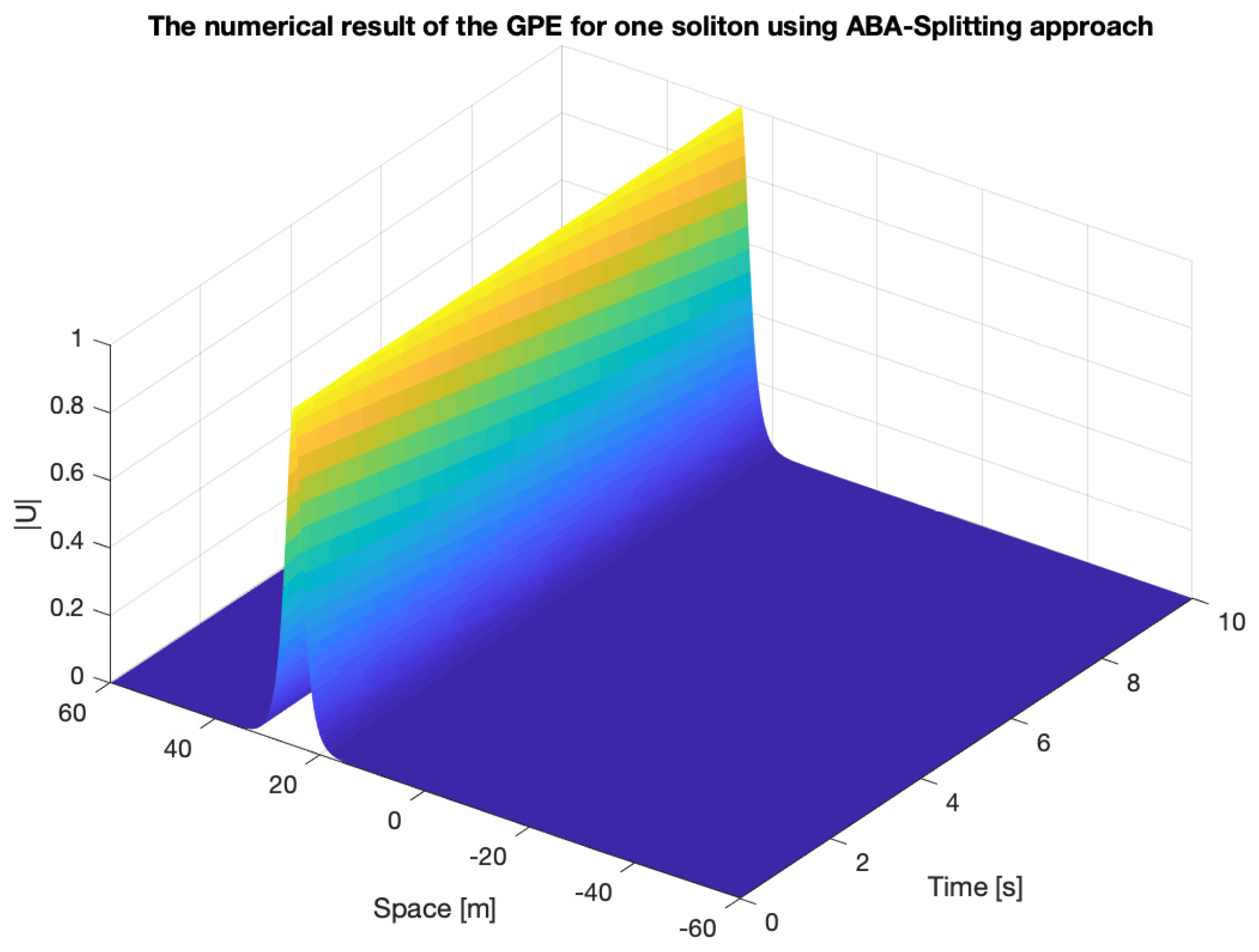
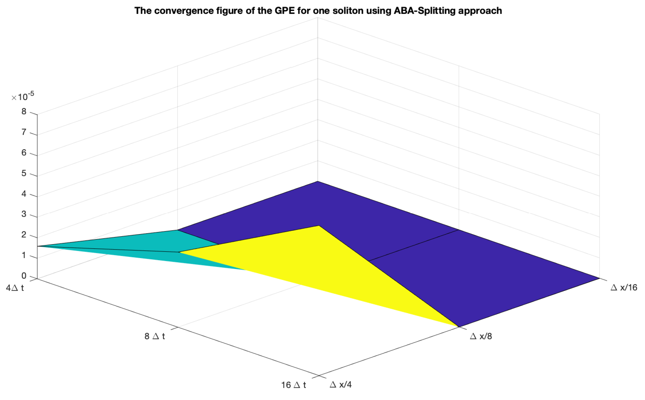
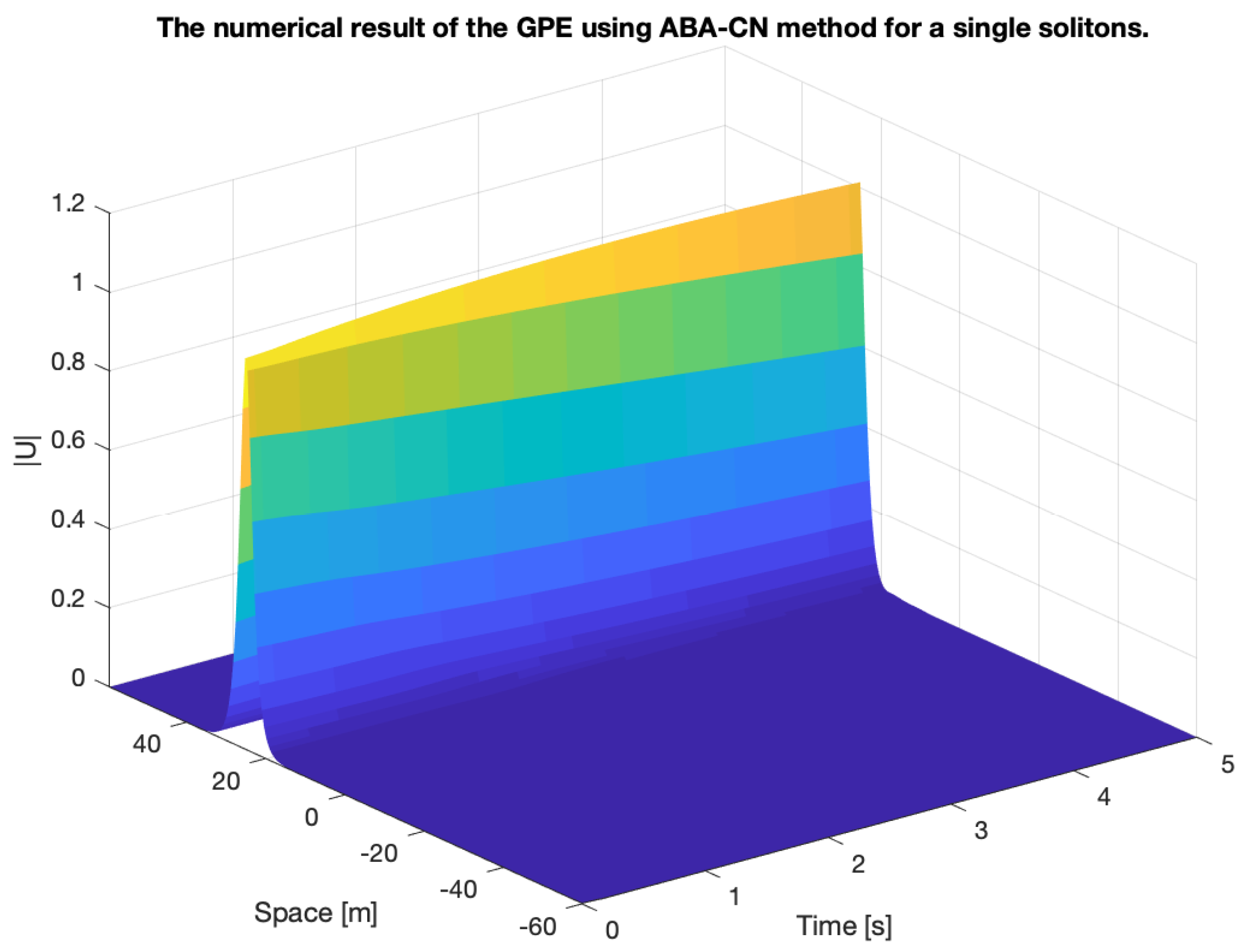
5.1. First Example: GPE with One Soliton

We consider the GPE to apply for the numerical schemes in a suitable rewriting:
u t = i H u , x Ω , t [ 0 , 1 ] ,
u ( x , 0 ) = sech ( 1 2 ( x 25 ) ) exp ( i x 20 ) , x Ω ,
u ( x , t ) = 0.0 , x Ω , t [ 0 , 1 ] ,
with H u = 1 2 2 x 2 + g | u | 2 σ u , σ = 1.0 and we have applied Dirichlet boundary conditions.
We applied for the analytical solution g = 1 , v d = 1 10 and v p = 199 200 and the analytical solution is given as:
u ( x , t ) = sech ( 1 2 ( x t 10 25 ) ) exp ( i ( x 20 199 400 t ) ) , ( x , t ) [ L , L ] × [ 0 , T ] .
We deal with the following methods:
  • Implicit Euler method (all operators are done with the implicit method),
  • Crank–Nicolson scheme (all operators are done with the CN method),
  • AB-splitting:
    -
    Linear operator is done with the Spectral method and nonlinear operator is done with the spectral method,
    -
    Linear operator is done with the FD method and nonlinear operator is done with the spectral method,
    -
    Linear operator is done with the Spectral method and nonlinear operator is done with the FD method,
    -
    Linear operator is done with the FD method and nonlinear operator is done with the FD method.
  • ABA-splitting:
    -
    Linear operator is done with the Spectral method and nonlinear operator is done with the spectral method.
  • ABA-CN and ABA-iCN:
    -
    Linear operator is done with the finite difference method, while the nonlinear operator is done with the spectral method.
    -
    For the iterative scheme, we apply different iterative steps.
The convergence-tableaus of the ABA-splitting and modified Crank–Nicolson methods are given in Table 1 and Table 2.
The computational times and the errors of the different methods for the single soliton solutions are given in Table 3 and Table 4.
Figure 1 presents the solutions of the one soliton results and the convergence tableau.
Figure 2 presents the solutions with the approximated conservation finite difference scheme.
Remark 11.
We see the benefits of the conservation schemes in the long time behaviour. But the drawbacks are the time-consuming computations. The balance based on the splitting approach including the conservative schemes are an alternative to reduce the time-consuming approaches and allow us to obtain asymptotic conservative results with sufficient iterative steps.

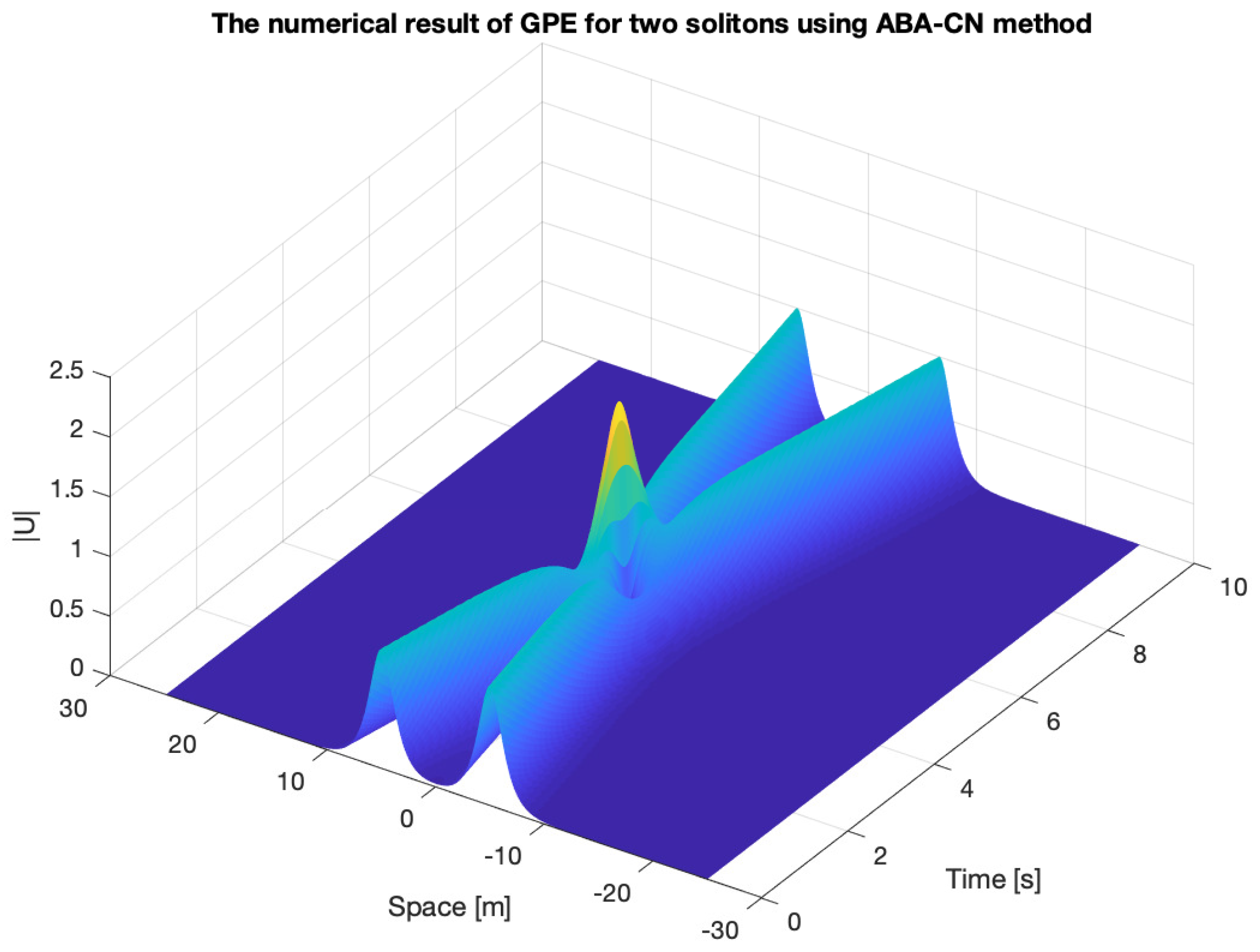
5.2. Second Example: Collision of Two Solitons

We apply a collision of two solitons with the GPE. The evolution equation is given as:
u t = i H u , x Ω , t [ 0 , 10 ] ,
u ( x , 0 ) = sech ( 1 2 ( x 20 ) ) exp ( i x 20 ) +
+ sech ( x + 20 ) exp ( i x 20 ) , x Ω ,
u ( x , t ) = 0.0 , x Ω , t [ 0 , T ] ,
with H u = 1 2 2 x 2 + g | u | 2 σ u , σ = 1.0 .
We have two solitons starting in x = 20 and x = 20 and they collide at x = 0 at the time-point t = 5.0 .
For the reference solution, we apply a fine spatial- and time-discretised solution with an ABA method.
Furthermore, we also decouple the full equation after the spatial discretisation into a linear and nonlinear operator part, given as:
H U n = A ( t , x , U n ) = A 1 ( t , x ) + A 2 ( t , x , U n ) ,
In Table 5 and Table 6, we present the computational time and the numerical errors of the different methods for the two-solitons modelling problem.
The solution of the two-solitons with the ABA-CN method in Figure 3.
Remark 12.
We also obtain the same results as for the single soliton solutions. The alternative methods with the combination of the conservative schemes and the splitting approaches have small numerical errors and optimal computational times in the area of the fast splitting methods. With additional iterative steps, we are able to better couple the ABA-iCN method and asymptotically achieve the conservation schemes.

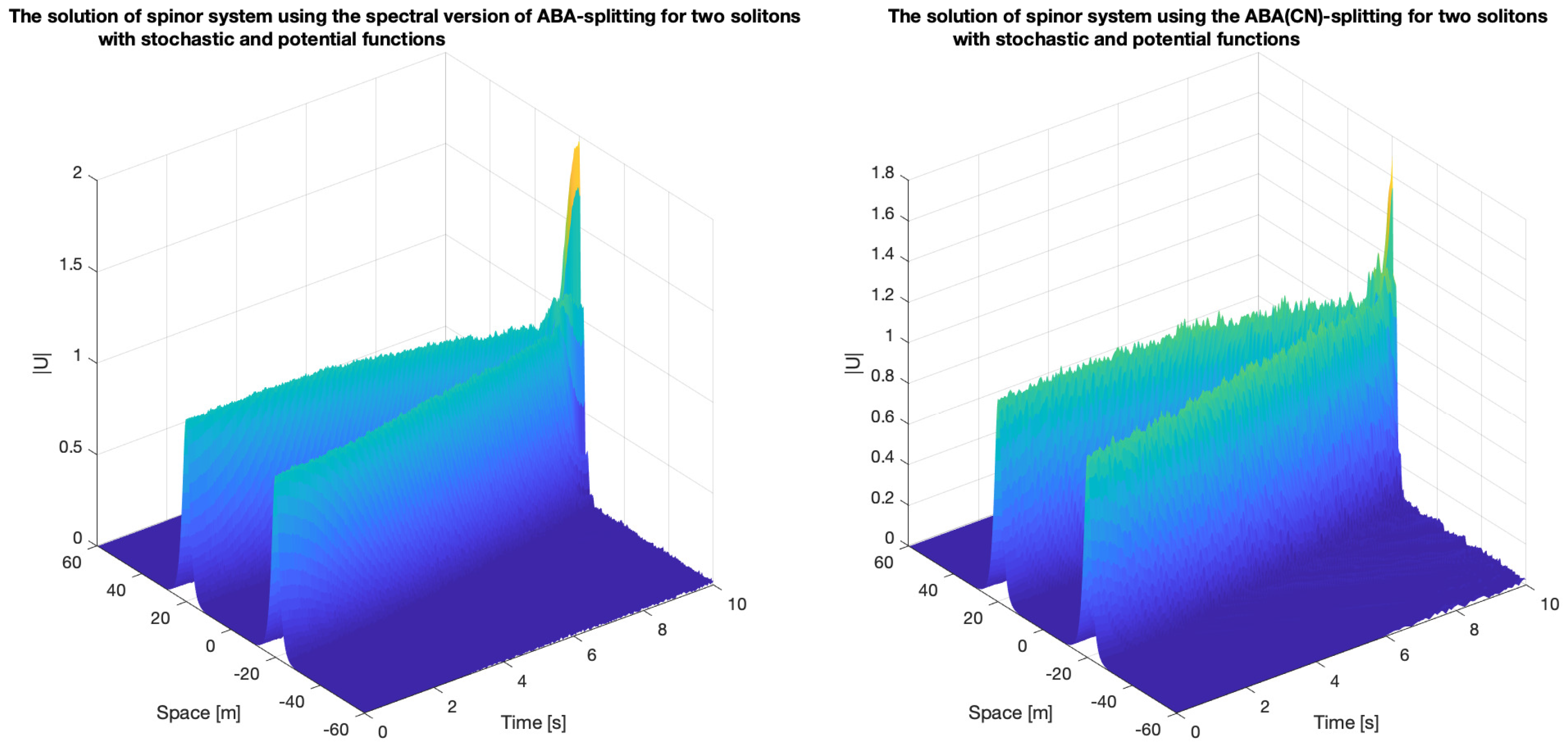
5.3. Spinor System (Coupled GPEs)

In the next experiment, we apply a vectorial system based on coupled GPEs. We deal with a coupled GPE, which is given as
u 1 t = i ( 1 2 2 u 1 x 2 g 1 , 1 | u 1 | 2 u 1 g 1 , 2 | u 2 | 2 u 1 ϵ p o t e n t i a l V ( x ) u 1 ϵ s t o c h d W d t u 1 ) , ( x , t ) [ L , L ] × [ 0 , T ] ,
u 2 t = i ( 1 2 2 u 2 x 2 g 2 , 1 | u 1 | 2 u 2 g 2 , 2 | u 2 | 2 u 2 ϵ p o t e n t i a l V ( x ) u 2 ϵ s t o c h d W d t u 2 ) , ( x , t ) [ L , L ] × [ 0 , T ] ,
where we assume g 1 , 1 = g 1 , 2 = g 2 , 1 = g 2 , 2 = 2 , where we have the boundary conditions u 1 ( x , t ) = u 2 ( x , t ) = 0 , x { L , L } , t [ 0 , T ] .
Furthermore, we apply ϵ p o t e n t i a l = 0.006 and ϵ s t o c h = 0.05 .
The initial conditions are given as:
  • Bright one-soliton:
    u 1 ( x , 0 ) = u 2 ( x , 0 ) = sech ( 1 2 ( x 25 ) ) exp ( i x 20 ) , x [ L , L ] .
  • Bright two-soliton:
    u 1 ( x , 0 ) = sech ( 1 2 ( x 20 ) ) exp ( i x 20 ) , x [ L , L ] ,
    u 2 ( x , 0 ) = sech ( 1 2 ( x + 20 ) ) exp ( i x 20 ) , x [ L , L ] .
The algorithms for the different splitting approach is given in Algorithms 9 and 10.
The results of the computational time and the numerical errors are given in Table 7, Table 8, Table 9 and Table 10.
The results of the spinor system with two soliton and the ABA-CN method methods are given in Figure 4, we apply e p s i l o n p o t e n t i a l = 0.05 and e p s i l o n s t o c h = 0.1 and also V ( x ) = x 2 .
Remark 13.
We also obtain the same benefits in the coupled GPEs, as for the scalar GPEs. The stable solutions of the modified Crank–Nicolson methods could be redone also in the vectorial cases.

6. Conclusions

We applied scalar and vectorial GPEs and extend the conservative finite difference schemes to vectorial applications. We propose an alternative ABA-iCN method, which combines the conservative finite difference scheme with a fast ABA splitting approaches. These alternative methods allow us to accelerate the solvers and stabilise the schemes to asymptotic conservative finite difference schemes. We apply different numerical test examples and verify our assumptions. In the future, we aim to carefully analyse the structure of the proposed methods with the underlying error analysis and present more real-life applications in the field of soliton collisions.

Author Contributions

The theory, the formal analysis and the methology presented in this paper was developped by J.G. The software development and the numerical validation of the methods was done by A.N. and with the help of J.G. The paper was written by J.G. and was corrected and edited by J.G. and A.N. The writing–review was done by J.G. The supervision and project administration was done by J.G.

Funding

This research was funded by German Academic Exchange Service grant number 91588469.

Acknowledgments

We acknowledge support by the DFG Open Access Publication Funds of the Ruhr-Universität of Bochum, Germany.

Conflicts of Interest

The authors declare no conflict of interest.

Appendix A

Appendix A.1. Proof for Continuous Mass-Conservation for the Deterministic Case

Proof. 
We have he L 2 -norm, which is given as:
N ( t ) = Ω i = 1 M | u i ( x , t ) | 2 d x ,
where we apply the time-derivation, which is given as:
N t = Ω t i = 1 M ˜ | u i ( x , t ) | 2 d x =
= Ω i = 1 M ˜ ( t u i · u i * + u i · t u i * ) d x =
= Ω i = 1 M ˜ ( i H u i · u i * + u i · H u i * ) d x = 0 .
where we apply the symmetry of H and we have N ( t ) = N ( 0 ) 0 . □
Remark A1.
The conservation laws are proved for the scalar GPE in Reference [8]. Therefore, we can also prove the impulse and energy conservation based on the proof of the mass conservation with respect to the additivity of the coupled system.

Appendix A.2. Proof for Discrete Mass-Conservation for the Deterministic Case

Proof. 
We have the L 2 -norm, which is given as:
N ¯ t = Δ x Δ t j = M M i = 1 M ˜ | u i , j n + 1 | 2 | u i , j n | 2 = Δ x j = M M i = 1 M ˜ u i , j n + 1 u t , i , j * , n + u i , j * , n u t , i , j n ,
where we apply the right hand side of the vectorial discretization scheme (19)–(21) and obtain:
N ¯ n + 1 N ¯ n = i Δ t Δ x j = M + 1 M 1 i = 1 M ˜ u i , j n + 1 u x x , i , j * , n + 1 + u x x , i , j * , n 2 + + 1 2 k = 1 M ˜ g ( | u k , j n + 1 | 2 + | u k , j n | 2 ) u i , j n + 1 u i , j * , n + u i , j * , n u x x , i , j n + 1 + u x x , i , j n 2 g 2 ( k = 1 M ˜ | u k , j n + 1 | 2 + | u k , j n | 2 ) u i , j n u i , j * , n =
= i Δ t Δ x 2 j = M + 1 M 1 i = 1 M ˜ 1 2 | u x , i , j n + 1 | 2 + g 2 ( k = 1 M ˜ | u k , j n + 1 | 2 ) | u i , j n + 1 | 2 1 2 | u x , i , j n | 2 + g 2 ( k = 1 M ˜ | u k , j n | 2 ) | u i , j n | 2 = i Δ t E ¯ n + 1 E ¯ n ,
where we obtain N ¯ n + 1 N ¯ n = 0 and E ¯ n + 1 E ¯ n = 0 for each n, see also the scalar case in Reference [8].
Therefore, we have N ¯ n = N ¯ 0 and E ¯ n = E ¯ 0 for each n, which means that we have proven the mass and energy conservation. □
Remark A2.
The discrete conservation laws for the CN scheme is proved for the scalar GPE in Reference [8]. Therefore, we can also prove the impulse conservation based on the proof of the mass conservation and energy conservation with respect to the additivity of the coupled system.
Remark A3.
The conservative behaviour of the semi-implicit Crank–Nicolson is proved in Reference [8].

References

  1. Dalfovo, F.; Giorgini, S.; Pitaevskii, L.P.; Stringari, S. Theory of Bose–Einstein condensation in trapped gases. Rev. Mod. Phys. 1999, 71, 463–512. [Google Scholar] [CrossRef]
  2. Abdullaev, F.K.; Gammal, A.; Kamchatnov, A.M.; Tomio, L. Dynamics of bright matter wave solitons in a Bose–Einstein condensate. Int. J. Mod. Phys. B 2005, 19, 3415–3473. [Google Scholar] [CrossRef]
  3. Dauxois, T.; Peyard, M. Physics of Solitons; Cambridge University Press: Cambridge, UK, 2006. [Google Scholar]
  4. Balakrishnan, R.; Satija, I.I. Solitons in Bose–Einstein condensates. Pramana J. Phys. 2011, 77, 929–947. [Google Scholar] [CrossRef]
  5. Kevrekidis, P.G.; Frantzeskakis, D.J.; Carretero-Gonzalez, R. Emergent Nonlinear Phenomena in Bose–Einstein Condensates Theory and Experiment; Springer Series on Atomic, Optical, and Plasma Physics; Springer: Heidelberg, Germany; New York, NY, USA, 2008. [Google Scholar]
  6. Shang, Y. Unveiling robustness and heterogeneity through percolation triggered by random-link breakdown. Phys. Rev. E 2014, 90, 032820. [Google Scholar] [CrossRef] [PubMed]
  7. Shang, Y. Effect of link oriented self-healing on resilience of networks. J. Stat. Mech. Theory Exp. 2016, 8, 083403. [Google Scholar] [CrossRef]
  8. Trofimov, V.A.; Peskov, N.V. Comparison of finite difference schemes for the Gross–Pitaevskii equation. Math. Model. Anal. 2009, 14, 109–126. [Google Scholar] [CrossRef]
  9. Atre, R.; Panigrahi, P.K.; Agarwal, G.S. Class of solitary wave solutions of the one-dimensional Gross–Pitaevskii equation. Phys. Rev. E 2006, 73, 056611. [Google Scholar] [CrossRef] [PubMed]
  10. Bao, W.; Cai, Y. Mathematical models and numerical methods for spinor Bose–Einstein condensates. Commun. Comput. Phys. 2018, 24, 899–965. [Google Scholar] [CrossRef]
  11. Bao, W.; Zhang, Y. Dynamical laws of the coupled Gross–Pitaevskii equations for spin-1 Bose–Einstein condensates. Methods Appl. Anal. 2010, 17, 49–80. [Google Scholar] [CrossRef]
  12. Jiang, S.; Wang, L.; Hong, J. Stochastic multi-symplectic integrator for stochastic nonlinear Schroedinger equation. Commun. Comput. Phys. 2013, 14, 393–411. [Google Scholar] [CrossRef]
  13. Antoine, X.; Bao, W.; Besse, C. Computational methods for the dynamics of the nonlinear Schrödinger and Gross–Pitaevskii equations. Comput. Phys. Commun. 2013, 184, 2621–2633. [Google Scholar] [CrossRef]
  14. Bao, W.; Cai, Y. Mathematical theory and numerical methods for Bose–Einstein condensation. Kinet. Relat. Mod. 2013, 6, 1–135. [Google Scholar] [CrossRef]
  15. Geiser, J. Iterative splitting method as almost asymptotic symplectic integrator for stochastic nonlinear Schrödinger equation. AIP Conf. Proc. 2017, 1863, 560005. [Google Scholar]
  16. Geiser, J. Multicomponent and Multiscale Systems: Theory, Methods, and Applications in Engineering; Springer: Cham, Switzerland; Heidelberg, Germany; New York, NY, USA; Dordrecht, The Netherlands; London, UK, 2016. [Google Scholar]
  17. Geiser, J.; Nasari, A. Simulation of Multiscale Schroedinger Equation with Extrapolated Splitting Approaches. In Proceedings of the AIP Conference, ICNAAM 2018, Rhodes, Greece, 13–18 September 2018. [Google Scholar]
  18. Ho, T.-L. Spinor Bose condensates in optical traps. Phys. Rev. Lett. 1998, 81, 742–745. [Google Scholar] [CrossRef]
  19. Takhtajan, L.A. Quantum Mechanics for Mathematicians; Graduate Series in Mathematics; American Mathematical Society: Providence, RI, USA, 2008; Volume 95. [Google Scholar]
  20. Bao, W.; Tang, Q.; Xu, Z. Numerical methods and comparison for computing dark and bright solitons in the nonlinear Schrödinger equation. J. Comput. Phys. 2013, 235, 423–445. [Google Scholar] [CrossRef]
  21. Bao, W.; Jaksch, D.; Markowich, P.A. Numerical solution of the Gross–Pitaevskii equation for Bose–Einstein condensation. J. Comput. Phys. 2003, 187, 318–342. [Google Scholar] [CrossRef]
  22. Min, B.; Li, T.; Rosenkranz, M.; Bao, W. Subdiffusive spreading of a Bose–Einstein condensate in random potentials. Phys. Rev. A 2012, 86, 053612. [Google Scholar] [CrossRef]
  23. Bao, W.; Cai, Y. Ground states of two-component Bose–Einstein condensates with an internal atomic Josephson junction. East Asia J. Appl. Math. 2011, 1, 49–81. [Google Scholar] [CrossRef]
  24. Bao, W.; Cai, Y.; Wang, H. Efficient numerical methods for computing ground states and dynamics of dipolar Bose–Einstein condensates. J. Comput. Phys. 2010, 229, 7874–7892. [Google Scholar] [CrossRef]
  25. Strang, G. On the construction and comparison of differential schemes. SIAM J. Numer. Anal. 1968, 5, 506–517. [Google Scholar] [CrossRef]
  26. Geiser, J. Iterative Splitting Methods for Differential Equations; Numerical Analysis and Scientific Computing Series; Taylor & Francis Group: Boca Raton, FL, USA; London, UK; New York, NY, USA, 2011. [Google Scholar]
  27. McLachlan, R.I.; Quispel, G.R.W. Splitting methods. Acta Numer. 2002, 11, 341–434. [Google Scholar] [CrossRef]
  28. Yan, Z.; Chow, K.W.; Malomed, B.A. Exact stationary wave patterns in three coupled nonlinear Schrödinger/Gross–Pitaevskii equations. Chaos Solitons Fract. 2009, 42, 3013–3019. [Google Scholar] [CrossRef]
  29. Brigham, E.O. The Fast Fourier Transform: An Introduction to Its Theory and Application; Prentice Hall: Upper Saddle River, NJ, USA, 1973. [Google Scholar]
Figure 1. Results of the GPEwith one soliton equation, here we have applied the ABA-splitting approach (upper figure: numerical results; lower figure: convergence results).
Mca 24 00076 g001aMca 24 00076 g001b
Figure 2. Numerical solution with the ABA-CN method of the single solitons.
Mca 24 00076 g002
Figure 3. Solution of the ABA-CN method for the two solitons.
Mca 24 00076 g003
Figure 4. Solution of the spinor system with two solitons with the stochastic and potential functions (left-hand figure: the results with the time-splitting method; right-hand figure: the results with the ABA-iCN method).
Mca 24 00076 g004
Table 1. Convergence tableau for the ABA-splitting method.
Δ x / 4 Δ x / 8 Δ x / 16
4 Δ t 1.593 × 10 5 4.216 × 10 10 2.211 × 10 12
8 Δ t 3.67 × 10 5 9.28 × 10 10 4.663 × 10 12
16 Δ t 7.34 × 10 5 1.855 × 10 9 9.326 × 10 12
Table 2. Convergence tableau for the ABA-CN-/ABA-iCN-splitting method.
Δ x / 4 Δ x / 8 Δ x / 16
4 Δ t 1.312 × 10 5 3.3337 × 10 10 1.6673 × 10 12
8 Δ t 3.667 × 10 5 9.2733 × 10 10 4.6629 × 10 12
16 Δ t 7.334 × 10 5 1.8547 × 10 9 9.3258 × 10 12
Table 3. Computational times of one soliton with the different methods.
T = 2.5T = 5T = 7.5T = 10
Implicit Euler method0.83131.67852.11242.9281
Crank–Nicolson scheme2.04963.89305.77647.1148
AB-splitting: A and B operators are spectral0.02710.04860.07850.1007
AB-splitting: A Spectral, B FD1.81593.21404.69325.7207
AB-splitting: A FD, B Spectral0.04660.05510.06680.0962
AB-splitting: A FD, B FD2.47983.82115.71467.0136
ABA-splitting0.03520.06320.09400.1264
BAB-splitting0.03430.06240.10030.1281
ABA(CN)-splitting0.97621.97742.61903.2304
ABA(semiCN)-splitting2.59064.59336.57658.5612
Table 4. Numerical errors of one soliton with the different methods.
T = 2.5T = 5T = 7.5T = 10
Implicit Euler method0.89771.90842.46162.6552
Crank–Nicolson scheme0.91652.02082.70692.9975
AB-splitting: A and B operators are spectral0.03300.03960.04200.0488
AB-splitting: A Spectral, B FD0.94432.04682.70542.9648
AB-splitting: A FD, B Spectral0.13330.38930.76501.2144
AB-splitting: A FD, B FD0.91652.02082.70692.9975
ABA-splitting0.00570.00800.00970.0111
BAB-splitting0.00570.00800.00970.0111
ABA(CN)-splitting0.91782.02012.69522.9630
ABA(semiCN)-splitting0.91742.02082.70032.9740
Table 5. Computational times of two solitons with the different methods.
T = 2.5T = 5T = 7.5T = 10
Implicit Euler method2.49283.56014.90316.2648
Crank–Nicolson scheme4.56488.892313.892615.9353
AB-splitting: A and B operators are spectral0.03420.06320.10040.1429
AB-splitting: A Spectral, B FD3.52926.73749.768312.9375
AB-splitting: A FD, B Spectral0.03490.06780.09650.1380
AB-splitting: A FD, B FD4.41828.599512.308616.4472
ABA-splitting0.04450.08580.14080.1989
BAB-splitting0.04250.07890.15240.1931
ABA(CN)-splitting2.18214.45676.38767.7092
ABA(semiCN)-splitting6.154310.521716.100719.6879
Table 6. Numerical errors of two solitons with the different methods.
T = 2.5T = 5T = 7.5T = 10
Implicit Euler method1.06054.64785.04865.1546
Crank–Nicolson scheme1.05484.37459.166619.2207
AB-splitting: A and B operators are spectral0.08660.10590.15010.1754
AB-splitting: A Spectral, B FD0.75791.84212.46542.8003
AB-splitting: A FD, B Spectral1.10016.041249.3173114.0526
AB-splitting: A FD, B FD1.05484.37459.166619.2207
ABA-splitting0.02960.03200.04100.0453
BAB-splitting0.02950.03140.04050.0447
ABA(CN)-splitting0.70241.84892.49492.7952
ABA(semiCN)-splitting0.85992.66452.77712.7894
Table 7. Computational times of one soliton in spinor system.
T = 2.5T = 5T = 7.5T = 10
ABA spectral method0.191170.380640.420710.54968
ABA (CN) method5.420710.804615.419619.7318
Table 8. Computational errors of one soliton in spinor system.
T = 2.5T = 5T = 7.5T = 10
ABA spectral method U193.1781117.8641131.5981135.3722
ABA spectral method U293.1308117.9896131.533135.7863
ABA spectral method U1 + U2186.2656235.8055263.0822271.0522
ABA (CN) method U192.9585118.1392132.451136.1172
ABA (CN) method U293.0261118.1044132.4937136.3657
ABA (CN) method U1 + U2185.8951235.9406264.3351271.7702
Table 9. Computational errors of two solitons in spinor system.
T = 2.5T = 5T = 7.5T = 10
ABA spectral method0.18780.375950.438020.53914
ABA (CN) method5.377710.783215.58219.9661
Table 10. Computational errors of two solitons in spinor system.
T = 2.5T = 5T = 7.5T = 10
ABA spectral method U122.674968.192795.2834113.0119
ABA spectral method U222.879468.01495.5527113.0438
ABA spectral method U1 + U232.211796.2128134.6855158.9924
ABA (CN) method U122.626466.796593.5702110.1788
ABA (CN) method U222.176566.53593.7642110.2908
ABA (CN) method U1 + U231.681594.2804132.3647155.4301

