A Novel Decision-Making Approach under Complex Pythagorean Fuzzy Environment

Abstract

A complex Pythagorean fuzzy set (CPFS) is an extension of a Pythagorean fuzzy set that is used to handle the vagueness with the degrees whose ranges are enlarged from real to complex subset with unit disc. In this research study, we propose the innovative concept of complex Pythagorean fuzzy graphs (CPFGs). Further, we present the concepts of regular and edge regular graphs in a complex Pythagorean fuzzy environment. Moreover, we develop a complex Pythagorean fuzzy graph based multi-attribute decision making an approach to handling the situations in which the graphic structure of attributes is obscure. A numerical example concerning information technology improvement project selection is utilized to illustrate the availability of the developed approach.

1. Introduction

The concept of Pythagorean fuzzy sets [1,2,3] is a relatively peculiar mathematical framework in the fuzzy family with a larger ability to deal with imprecision and obscurity in decision-making. The Pythagorean fuzzy model relaxes the condition $\mu +\nu \le 1$ with ${\mu }^2+{\nu }^2\le 1$ and has higher potentiality than intuitionistic fuzzy sets (IFSs) [4] to manage the complex obscurity in practical decision making problems. Ramot et al. [5] put forward the concept of a complex fuzzy set (CFS) by extending the range of membership function from real to complex number with the unit disc. Yazdanbakhsh and Dick [6] provided a systematic review of CFSs. After the inception of CFS by Ramot et al., several researchers [6,7,8] divert their attention to CFSs. Later, Alkouri and Salleh [9,10] generalized the concept of CFS to complex intuitionistic fuzzy sets (CIFSs) by representing the degree of complex valued non-membership functions and proposed the concepts of complex intuitionistic fuzzy relation and a distance measure under a CIFS environment. Rani and Garg [11] investigated some series of distance measures between the two CIFSs, presented the complex intuitionistic fuzzy power aggregation operators [12], generalized complex intuitionistic fuzzy aggregation operators [13] and provided their applications in the process of decision-making. Kumar and Bajaj [14] introduced some distance and entropy measures in complex intuitionistic fuzzy soft circumstances. PFS can only handle the vagueness and uncertainty that exist in the data but is unable to show the partial ignorance of the information and its fluctuations at a specific phase of time during their execution. Moreover, in real life, vagueness and uncertainty presenting in the data occur concurrently with changes to the phase (periodicity) of the data. Thus, to consider this information, the existing theories are insufficient and hence, some information loss during the process. To overthrow it, Ullah et al. [15] introduced the notion of CPFSs and extended some distance measures to accommodate complex Pythagorean fuzzy values.

A graph is a model of relations and is a convenient tool for depicting information comprising a relationship between objects. In networking, due to the development of system complexity, a variety of uncertain information is frequently encountered. To handle this vague or uncertain information, Rosenfeld [16] put forward the notion of fuzzy graphs. Mordeson and Peng [17] defined the operations on graphs within fuzzy contexts. Yu and Xu [18] developed the graph based multi-attribute decision-making model, to solve MADM problems with the interrelated attributes. With the more obscure information in the networks, several generalizations of fuzzy graphs [19,20] have been put forward by many researchers. Naz et al. [21] emanated the concept of Pythagorean fuzzy graphs (PFGs). Later, Akram et al. [22,23,24] proposed certain novel concepts of graphs under a Pythagorean fuzzy environment. Akram et al. [25] simplify the expressions of an interval-valued Pythagorean fuzzy set by providing a new idea of a simplified interval-valued Pythagorean fuzzy set and originally put forward the notion of simplified interval-valued Pythagorean fuzzy graph along its applications in decision making. In the existing theories of fuzzy graph and its generalization, the vagueness present in the data and its relations are managed with the aid of membership and non-membership degrees which are the subset of real numbers and may give up some effective information. An alternative to these, CFS handles the uncertainties with the degrees whose ranges are extended from the real subset to the complex subset with unit disc and hence handle the two-dimensional information in a single set. To utilize this benefit, Thirunavukarasu et al. [26] put forward the concept of complex fuzzy graphs. Yaqoob et al. [27] introduced the concept of complex intuitionistic fuzzy graph with its application in cellular network provider companies. Further, Yaqoob and Akram [28] extended the concept of complex fuzzy graphs to complex neutrosophic graphs. As CPFS is a more generalized version of the existing theories such as FSs, IFSs, CFSs and CIFSs. Thus, motivated by this, in this paper, within complex Pythagorean fuzzy contexts, we introduce the innovative concept of complex Pythagorean fuzzy graphs (CPFGs) in which pairs of the membership degrees represent the two-dimensional information. We develop operations on two CPFGs and investigate their desirable properties. We define the concepts of regular and edge regular graphs with appropriate illustration and examine some of their crucial properties with complex Pythagorean fuzzy information. Aggregation operators have great importance in many fields of information processing such as decision making, medical diagnosis, pattern recognition, data mining machine retrieval and machine learning, and so forth. Aggregation operators are commonly used to convert all the inputted individual information into a single value. So, we also develop systematic operations and aggregation operators to aggregate complex Pythagorean fuzzy information. Finally, we develop a CPFG based MADM approach to handle situations in which the attributes graphic structure is uncertain.

The paper is structured as follows: Section 2 proposes a new generalization of Pythagorean fuzzy graphs—called CPFG—and investigates its properties in detail. Section 3 discusses the edge regularity of a graph in complex Pythagorean fuzzy circumstances. In Section 4, we discuss the aggregation operators of CPFSs and provide the application of CPFSs and CPFGs in MADM and finally we draw conclusions and elaborate on future work in Section 5.

Definition 1

([15]). Let Y be the universe of discourse. A complex Pythagorean fuzzy set $\mathcal{C}$ defined on Y is an object of the form

$$\mathcal{C}=\{(r,{\mu }_{\mathcal{C}}\left(r\right)e^{i{\alpha }_{\mathcal{C}}\left(r\right)},{\nu }_{\mathcal{C}}\left(r\right)e^{i{\beta }_{\mathcal{C}}\left(r\right)}):r\in Y\},$$

where $i=\sqrt{-1},{\mu }_{\mathcal{C}}\left(r\right),{\nu }_{\mathcal{C}}\left(r\right)\in [0,1]$, ${\alpha }_{\mathcal{C}}\left(r\right),{\beta }_{\mathcal{C}}\left(r\right)\in [0,2\pi ]$, $0\le {\mu }_{\mathcal{C}}^2\left(r\right)+{\nu }_{\mathcal{C}}^2\left(r\right)\le 1$ and $0\le {\alpha }_{\mathcal{C}}^2\left(r\right)+{\beta }_{\mathcal{C}}^2\left(r\right)\le 2\pi$.

Definition 2

([15]). Let $\mathcal{C}=\{(r,{\mu }_{\mathcal{C}}\left(r\right)e^{i{\alpha }_{\mathcal{C}}\left(r\right)},{\nu }_{\mathcal{C}}\left(r\right)e^{i{\beta }_{\mathcal{C}}\left(r\right)}):r\in Y\},$${\mathcal{C}}_1=\{(r,{\mu }_{{\mathcal{C}}_1}\left(r\right)e^{i{\alpha }_{{\mathcal{C}}_1}\left(r\right)},{\nu }_{{\mathcal{C}}_1}\left(r\right)e^{i{\beta }_{{\mathcal{C}}_1}\left(r\right)}):r\in Y\},$ and ${\mathcal{C}}_2=\{(r,{\mu }_{{\mathcal{C}}_2}\left(r\right)e^{i{\alpha }_{{\mathcal{C}}_2}\left(r\right)},{\nu }_{{\mathcal{C}}_2}\left(r\right)e^{i{\beta }_{{\mathcal{C}}_2}\left(r\right)}):r\in Y\}$ be the three CPFSs in Y, then

(i) 

${\mathcal{C}}_1\subseteq {\mathcal{C}}_2$ if and only if ${\mu }_{{\mathcal{C}}_1}\left(r\right)\le {\mu }_{{\mathcal{C}}_2}\left(r\right),{\nu }_{{\mathcal{C}}_1}\left(r\right)\ge {\nu }_{{\mathcal{C}}_2}\left(r\right)$ for amplitude terms and ${\alpha }_{{\mathcal{C}}_1}\left(r\right)\le {\alpha }_{{\mathcal{C}}_2}\left(r\right)$, ${\beta }_{{\mathcal{C}}_1}\left(r\right)\ge {\beta }_{{\mathcal{C}}_2}\left(r\right)$ for phase terms, for all $r\in Y$;

(ii) 

${\mathcal{C}}_1={\mathcal{C}}_2$ if and only if ${\mu }_{{\mathcal{C}}_1}\left(r\right)={\mu }_{{\mathcal{C}}_2}\left(r\right),{\nu }_{{\mathcal{C}}_1}\left(r\right)={\nu }_{{\mathcal{C}}_2}\left(r\right)$ for amplitude terms and ${\alpha }_{{\mathcal{C}}_1}\left(r\right)={\alpha }_{{\mathcal{C}}_2}\left(r\right)$, ${\beta }_{{\mathcal{C}}_1}\left(r\right)={\beta }_{{\mathcal{C}}_2}\left(r\right)$ for phase terms, for all $r\in Y$;

(iii) 

$\overline{\mathcal{C}}=\{(r,{\nu }_{\mathcal{C}}\left(r\right)e^{i{\beta }_{\mathcal{C}}\left(r\right)},{\mu }_{\mathcal{C}}\left(r\right)e^{i{\alpha }_{\mathcal{C}}\left(r\right)}):r\in Y\}.$

For simplicity, the pair $(\mu e^{i\alpha },\nu e^{i\beta })$ is called the complex Pythagorean fuzzy number (CPFN), where $\mu ,\nu \in [0,1]$ such that ${\mu }^2+{\nu }^2\le 1$ and $\alpha ,\beta \in [0,2\pi ]$ such that $0\le {\alpha }^2+{\beta }^2\le 2\pi$.

Example 1.

Suppose a fixed set Y contains only one element r, ${\mu }_{\mathcal{C}}\left(r\right)=0.4,{\alpha }_{\mathcal{C}}\left(r\right)=1.2\pi ,{\nu }_{\mathcal{C}}\left(r\right)=0.7,{\beta }_{\mathcal{C}}\left(r\right)=1.6\pi .$ Then $\mathcal{C}=\left\{(r,0.4e^{i2\pi \left(0.6\right)},0.7e^{i2\pi \left(0.8\right)})\right\}$ is a CPFN and denoted by $\mathcal{C}=(0.4e^{i2\pi \left(0.6\right)},0.7e^{i2\pi \left(0.8\right)})$ for simplicity.

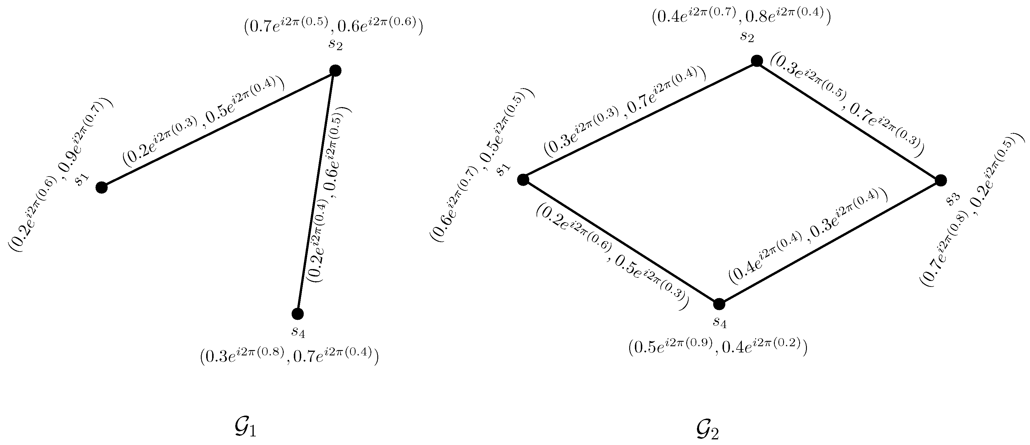
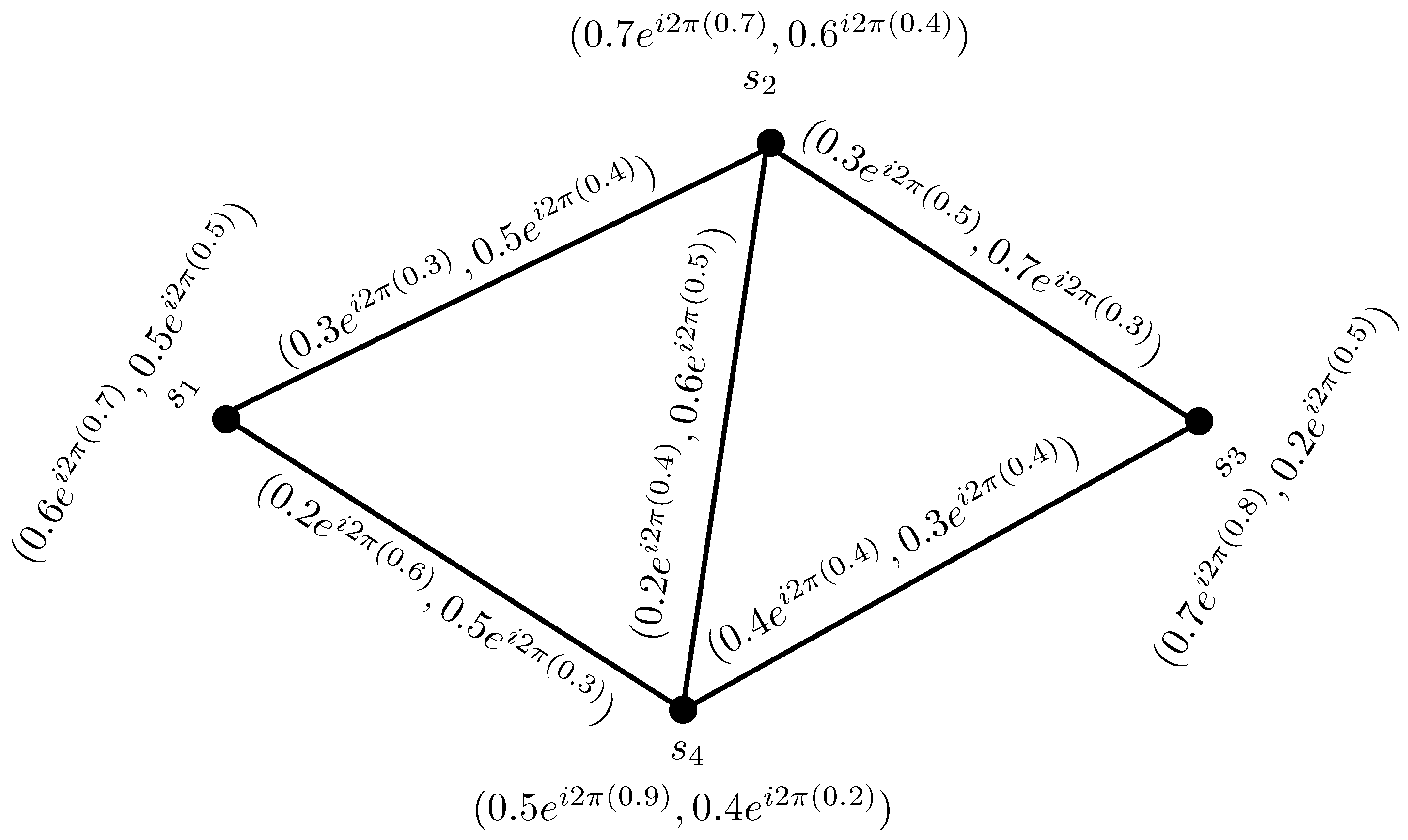
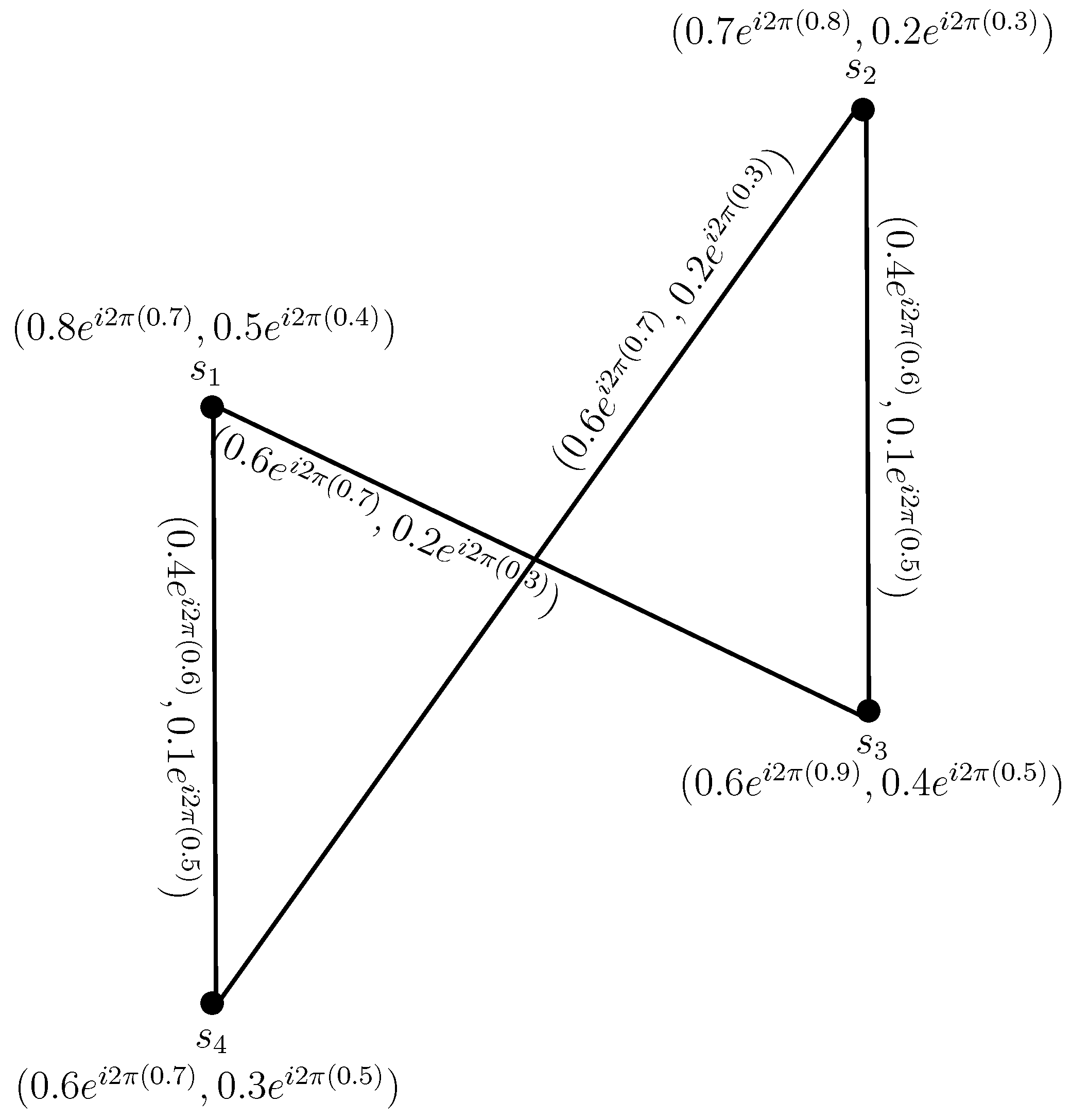
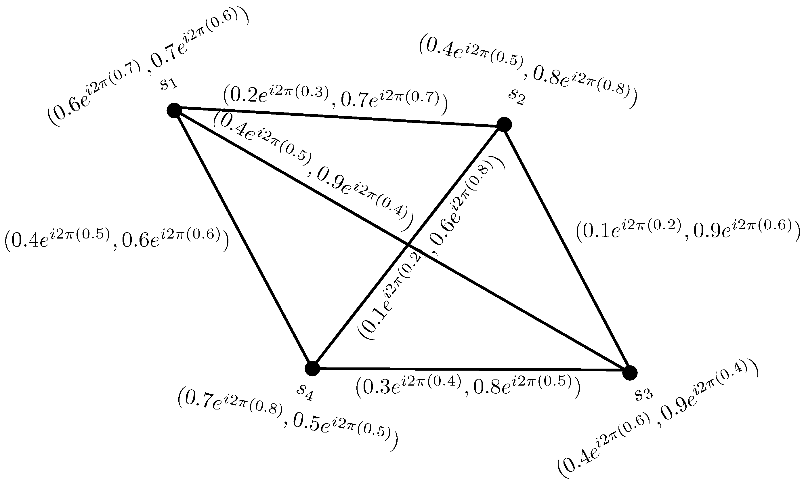
2. Graphs in Complex Pythagorean Fuzzy Environment

In this section, the innovative concepts of complex Pythagorean fuzzy relation and CPFG are introduced and some related properties are investigated.

Definition 3.

Let ${\mathcal{C}}_1=\{(r,{\mu }_{{\mathcal{C}}_1}\left(r\right)e^{i{\alpha }_{{\mathcal{C}}_1}\left(r\right)},{\nu }_{{\mathcal{C}}_1}\left(r\right)e^{i{\beta }_{{\mathcal{C}}_1}\left(r\right)}):r\in Y\},$ and ${\mathcal{C}}_2=\{(r,{\mu }_{{\mathcal{C}}_2}\left(r\right)e^{i{\alpha }_{{\mathcal{C}}_2}\left(r\right)},{\nu }_{{\mathcal{C}}_2}\left(r\right)e^{i{\beta }_{{\mathcal{C}}_2}\left(r\right)}):r\in Y\}$ be two CPFSs in Y, then

(i) 

${\mathcal{C}}_1\cup {\mathcal{C}}_2=\left\{\left(r,({\mu }_{{\mathcal{C}}_1}\left(r\right)\vee {\mu }_{{\mathcal{C}}_2}\left(r\right))e^{i({\alpha }_{{\mathcal{C}}_1}\left(r\right)\vee {\alpha }_{{\mathcal{C}}_2}\left(r\right))},({\nu }_{{\mathcal{C}}_1}\left(r\right)\wedge {\nu }_{{\mathcal{C}}_2}\left(r\right))e^{i({\beta }_{{\mathcal{C}}_1}\left(r\right)\wedge {\beta }_{{\mathcal{C}}_2}\left(r\right))}\right):r\in Y\right\}$;

(ii) 

${\mathcal{C}}_1\cap {\mathcal{C}}_2=\left\{\left(r,({\mu }_{{\mathcal{C}}_1}\left(r\right)\wedge {\mu }_{{\mathcal{C}}_2}\left(r\right))e^{i({\alpha }_{{\mathcal{C}}_1}\left(r\right)\wedge {\alpha }_{{\mathcal{C}}_2}\left(r\right))},({\nu }_{{\mathcal{C}}_1}\left(r\right)\vee {\nu }_{{\mathcal{C}}_2}\left(r\right))e^{i({\beta }_{{\mathcal{C}}_1}\left(r\right)\vee {\beta }_{{\mathcal{C}}_2}\left(r\right))}\right):r\in Y\right\}$.

Definition 4.

A CPFS $\mathcal{D}$ in $Y\times Y$ is said to be a complex Pythagorean fuzzy relation in Y, characterized by

$$\mathcal{D}=\left\{\langle rs,{\mu }_{\mathcal{D}}\left(rs\right)e^{i{\alpha }_{\mathcal{D}}\left(rs\right)},{\nu }_{\mathcal{D}}\left(rs\right)e^{i{\beta }_{\mathcal{D}}\left(rs\right)}\rangle \right|rs\in Y\times Y\},$$

where ${\mu }_{\mathcal{D}}:Y\times Y\to [0,1]$ and ${\nu }_{\mathcal{D}}:Y\times Y\to [0,1]$ depict the membership and non-membership function of $\mathcal{D}$, respectively, such that $0\le {\mu }_{\mathcal{D}}^2\left(rs\right)+{\nu }_{\mathcal{D}}^2\left(rs\right)\le 1$ and $0\le {\alpha }_{\mathcal{D}}^2\left(rs\right)+{\beta }_{\mathcal{D}}^2\left(rs\right)\le 2\pi$ for all $rs\in Y\times Y.$

Definition 5.

A complex Pythagorean fuzzy graph on a non-empty set Y is a pair $\mathcal{G}=(\mathcal{C},\mathcal{D})$, where $\mathcal{C}$ is a complex Pythagorean fuzzy set on Y and $\mathcal{D}$ is a complex Pythagorean fuzzy relation on Y such that:

$$\begin{array}{c}{\mu }_{\mathcal{D}}\left(rs\right)e^{i{\alpha }_{\mathcal{D}}\left(rs\right)}\le ({\mu }_{\mathcal{C}}\left(r\right)\wedge {\mu }_{\mathcal{C}}\left(s\right))e^{i({\alpha }_{\mathcal{C}}\left(r\right)\wedge {\alpha }_{\mathcal{C}}\left(s\right))},\hfill \\ {\nu }_{\mathcal{D}}\left(rs\right)e^{i{\beta }_{\mathcal{D}}\left(rs\right)}\le ({\nu }_{\mathcal{C}}\left(r\right)\vee {\nu }_{\mathcal{C}}\left(s\right))e^{i({\beta }_{\mathcal{C}}\left(r\right)\vee {\beta }_{\mathcal{C}}\left(s\right))}\hfill \end{array}$$

$0\le {\mu }_{\mathcal{D}}^2\left(rs\right)+{\nu }_{\mathcal{D}}^2\left(rs\right)\le 1$ and $0\le {\alpha }_{\mathcal{D}}^2\left(rs\right)+{\beta }_{\mathcal{D}}^2\left(rs\right)\le 2\pi$ for all $r,s\in Y.$ We call $\mathcal{C}$ and $\mathcal{D}$ the complex Pythagorean fuzzy vertex set and the complex Pythagorean fuzzy edge set of $\mathcal{G}$, respectively.

Example 2.

Consider a graph $G=(C,D)$, where $C=\{s_1,s_2,s_3,s_4,s_5\}$ is the vertex set and $D=\{s_1{s}_2,s_2{s}_3,s_3{s}_4,s_1{s}_5,s_2{s}_5,s_3{s}_5,s_4{s}_5\}$ is the edge set of G. Let $\mathcal{G}=(\mathcal{C},\mathcal{D})$ be a CPFG on C, as given in Figure 1, defined by:

$$\begin{array}{ccc}\hfill \mathcal{C}& =& 〈\left(\frac{s_1}{0.5e^{i2\pi \left(0.7\right)}},\frac{s_2}{0.8e^{i2\pi \left(0.8\right)}},\frac{s_3}{0.7e^{i2\pi \left(0.9\right)}},\frac{s_4}{0.4e^{i2\pi \left(0.6\right)}},\frac{s_5}{0.8e^{i2\pi \left(0.9\right)}}\right),\hfill \\ & & \left(\frac{s_1}{0.6e^{i2\pi \left(0.4\right)}},\frac{s_2}{0.3e^{i2\pi \left(0.6\right)}},\frac{s_3}{0.4e^{i2\pi \left(0.3\right)}},\frac{s_4}{0.3e^{i2\pi \left(0.5\right)}},\frac{s_5}{0.5e^{i2\pi \left(0.3\right)}}\right)〉,\hfill \\ \hfill \mathcal{D}& =& 〈\left(\frac{s_1{s}_2}{0.5e^{i2\pi \left(0.6\right)}},\frac{s_2{s}_3}{0.6e^{i2\pi \left(0.4\right)}},\frac{s_3{s}_4}{0.4e^{i2\pi \left(0.3\right)}},\frac{s_1{s}_5}{0.4e^{i2\pi \left(0.6\right)}},\frac{s_2{s}_5}{0.7e^{i2\pi \left(0.3\right)}},\frac{s_3{s}_5}{0.6e^{i2\pi \left(0.8\right)}},\frac{s_4{s}_5}{0.3e^{i2\pi \left(0.5\right)}}\right),\hfill \\ & & \left(\frac{s_1{s}_2}{0.6e^{i2\pi \left(0.5\right)}},\frac{s_2{s}_3}{0.2e^{i2\pi \left(0.5\right)}},\frac{s_3{s}_4}{0.2e^{i2\pi \left(0.4\right)}},\frac{s_1{s}_5}{0.6e^{i2\pi \left(0.2\right)}},\frac{s_2{s}_5}{0.4e^{i2\pi \left(0.5\right)}},\frac{s_3{s}_5}{0.4e^{i2\pi \left(0.3\right)}},\frac{s_4{s}_5}{0.4e^{i2\pi \left(0.4\right)}}\right)〉.\hfill \end{array}$$

To compare the CPFGs with PFGs, we convert the vertex set and the edge set of CPFG in Figure 1, from complex Pythagorean fuzzy numbers to the Pythagorean fuzzy numbers by considering the phase terms of each complex Pythagorean fuzzy value as zero, as shown in Figure 2.

The proposed extended fuzzy graph—named CPFG—is more rational to reality in the process of decision-making. In PFG, the information consists of a real-valued membership and non-membership degrees and just considers the amplitude term, which causes loss of information. Further, a CPFG is an extension of the existing theories such as fuzzy graphs, complex fuzzy graphs [26] and PFGs [21] by considering more or more information related to the vertices and relations and to deal with the two-dimensional information in a single set.

Definition 6.

Let $\mathcal{C}=\left\{(r,{\mu }_{\mathcal{C}}\left(r\right)e^{i{\alpha }_{\mathcal{C}}\left(r\right)},{\nu }_{\mathcal{C}}\left(r\right)e^{i{\beta }_{\mathcal{C}}\left(r\right)})\right|r\in C\}$ and $\mathcal{D}=\left\{(rs,{\mu }_{\mathcal{D}}\left(rs\right)e^{i{\alpha }_{\mathcal{D}}\left(rs\right)},{\nu }_{\mathcal{D}}\left(rs\right)e^{i{\beta }_{\mathcal{D}}\left(rs\right)})\right|rs\in D\}$ be the vertex and the edge set of a CPFG $\mathcal{G}$, then the order of a CPFG $\mathcal{G}$ is denoted by $O\left(\mathcal{G}\right)$ and is defined as:

$$O\left(\mathcal{G}\right)=\left({\displaystyle \sum _{r_i\in C}}{\mu }_{\mathcal{C}}\left(r_i\right)e^{i{\displaystyle \sum _{r_i\in C}}{\alpha }_{\mathcal{C}}\left(r_i\right)},{\displaystyle \sum _{r_i\in C}}{\nu }_{\mathcal{C}}\left(r_i\right)e^{i{\displaystyle \sum _{r_i\in C}}{\beta }_{\mathcal{C}}\left(r_i\right)}\right).$$

The size of a CPFG $\mathcal{G}$ is denoted by $S\left(\mathcal{G}\right)$ and is defined as:

$$S\left(\mathcal{G}\right)=\left({\displaystyle \sum _{r_i{r}_j\in D}}{\mu }_{\mathcal{D}}\left(r_i{r}_j\right)e^{i{\displaystyle \sum _{r_i{r}_j\in D}}{\alpha }_{\mathcal{D}}\left(r_i{r}_j\right)},{\displaystyle \sum _{r_i{r}_j\in D}}{\nu }_{\mathcal{D}}\left(r_i{r}_j\right)e^{i{\displaystyle \sum _{r_i{r}_j\in D}}{\beta }_{\mathcal{D}}\left(r_i{r}_j\right)}\right).$$

Example 3.

The order and size of the CPFG given in Figure 1 is $O\left(\mathcal{G}\right)=(3.2e^{i2\pi \left(3.9\right)},2.1{}^{i2\pi \left(2.1\right)})$ and $S\left(\mathcal{G}\right)=(3.5e^{i2\pi \left(3.5\right)},2.8{}^{i2\pi \left(2.8\right)})$, respectively.

Definition 7.

The complement of a CPFG $\mathcal{G}=(\mathcal{C},\mathcal{D})$ on an underlying graph $G=(C,D)$ is a CPFG $\overline{\mathcal{G}}=(\overline{\mathcal{C}},\overline{\mathcal{D}})$ defined by

1. 

$\overline{{\mu }_{\mathcal{C}}\left(r\right)e^{i{\alpha }_{\mathcal{C}}\left(r\right)}}={\mu }_{\mathcal{C}}\left(r\right)e^{i{\alpha }_{\mathcal{C}}\left(r\right)}$ and $\overline{{\nu }_{\mathcal{C}}\left(r\right)e^{i{\beta }_{\mathcal{C}}\left(r\right)}}={\nu }_{\mathcal{C}}\left(r\right)e^{i{\beta }_{\mathcal{C}}\left(r\right)}.$

2. 

$\overline{{\mu }_{\mathcal{D}}\left(rs\right)e^{i{\alpha }_{\mathcal{D}}\left(rs\right)}}=\left\{\begin{array}{cc}\left({\mu }_{\mathcal{C}}\left(r\right)\wedge {\mu }_{\mathcal{C}}\left(s\right)\right)e^{i({\alpha }_{\mathcal{C}}\left(r\right)\wedge {\alpha }_{\mathcal{C}}\left(s\right))}\hfill & \mathrm{if}{\mu }_{\mathcal{D}}\left(rs\right)e^{i{\alpha }_{\mathcal{D}}\left(rs\right)}=0,\hfill \\ \left({\mu }_{\mathcal{C}}\left(r\right)\wedge {\mu }_{\mathcal{C}}\left(s\right)\right)e^{i({\alpha }_{\mathcal{C}}\left(r\right)\wedge {\alpha }_{\mathcal{C}}\left(s\right))}-{\mu }_{\mathcal{D}}\left(rs\right)e^{i{\alpha }_{\mathcal{D}}\left(rs\right)}\hfill & \mathrm{if}0<{\mu }_{\mathcal{D}}\left(rs\right)e^{i{\alpha }_{\mathcal{D}}\left(rs\right)}\le 1.\hfill \end{array}\right.$

$\overline{{\nu }_{\mathcal{D}}\left(rs\right)e^{i{\beta }_{\mathcal{D}}\left(rs\right)}}=\left\{\begin{array}{cc}({\nu }_{\mathcal{C}}\left(r\right)\vee {\nu }_{\mathcal{C}}\left(s\right))e^{i({\beta }_{\mathcal{C}}\left(r\right)\vee {\beta }_{\mathcal{C}}\left(s\right))}\hfill & \mathrm{if}{\nu }_{\mathcal{D}}\left(rs\right)e^{i{\beta }_{\mathcal{D}}\left(rs\right)}=0,\hfill \\ ({\nu }_{\mathcal{C}}\left(r\right)\vee {\nu }_{\mathcal{C}}\left(s\right))e^{i({\beta }_{\mathcal{C}}\left(r\right)\vee {\beta }_{\mathcal{C}}\left(s\right))}-{\nu }_{\mathcal{D}}\left(rs\right)e^{i{\beta }_{\mathcal{D}}\left(rs\right)}\hfill & \mathrm{if}0<{\nu }_{\mathcal{D}}\left(rs\right)e^{i{\beta }_{\mathcal{D}}\left(rs\right)}\le 1.\hfill \end{array}\right.$

Example 4.

Consider a CPFG $\mathcal{G}=(\mathcal{C},\mathcal{D})$ on $C=\{s_1,s_2,s_3,s_4\}$, as in Figure 3, defined by:

$$\begin{array}{ccc}\hfill \mathcal{C}& =& 〈\left(\frac{s_1}{0.7e^{i2\pi \left(0.8\right)}},\frac{s_2}{0.8e^{i2\pi \left(0.7\right)}},\frac{s_3}{0.6e^{i2\pi \left(0.6\right)}},\frac{s_4}{0.9e^{i2\pi \left(0.7\right)}}\right),\left(\frac{s_1}{0.4e^{i2\pi \left(0.6\right)}},\frac{s_2}{0.3e^{i2\pi \left(0.5\right)}},\frac{s_3}{0.5e^{i2\pi \left(0.3\right)}},\frac{s_4}{0.2e^{i2\pi \left(0.4\right)}}\right)〉,\hfill \\ \hfill \mathcal{D}& =& 〈\left(\frac{s_1{s}_4}{0.2e^{i2\pi \left(0.4\right)}},\frac{s_2{s}_4}{0.8e^{i2\pi \left(0.7\right)}},\frac{s_3{s}_4}{0.3e^{i2\pi \left(0.2\right)}}\right),\left(\frac{s_1{s}_4}{0.3e^{i2\pi \left(0.5\right)}},\frac{s_2{s}_4}{0.3e^{i2\pi \left(0.5\right)}},\frac{s_3{s}_4}{0.4e^{i2\pi \left(0.3\right)}}\right)〉.\hfill \end{array}$$

Utilizing Definition 7, complement of a CPFG can be obtained, as given in Figure 4, and defined by:

$$\begin{array}{ccc}\hfill \overline{\mathcal{C}}& =& 〈\left(\frac{s_1}{0.7e^{i2\pi \left(0.8\right)}},\frac{s_2}{0.8e^{i2\pi \left(0.7\right)}},\frac{s_3}{0.6e^{i2\pi \left(0.6\right)}},\frac{s_4}{0.9e^{i2\pi \left(0.7\right)}}\right),\left(\frac{s_1}{0.4e^{i2\pi \left(0.6\right)}},\frac{s_2}{0.3e^{i2\pi \left(0.5\right)}},\frac{s_3}{0.5e^{i2\pi \left(0.3\right)}},\frac{s_4}{0.2e^{i2\pi \left(0.4\right)}}\right)〉,\hfill \\ \hfill \overline{\mathcal{D}}& =& 〈\left(\frac{s_1{s}_4}{0.5e^{i2\pi \left(0.3\right)}},\frac{s_3{s}_4}{0.3e^{i2\pi \left(0.4\right)}},\frac{s_1{s}_2}{0.7e^{i2\pi \left(0.7\right)}},\frac{s_2{s}_3}{0.6e^{i2\pi \left(0.6\right)}},\frac{s_3{s}_1}{0.6e^{i2\pi \left(0.6\right)}}\right),\hfill \\ & & \left(\frac{s_1{s}_4}{0.1e^{i2\pi \left(0.1\right)}},\frac{s_3{s}_4}{0.1e^{i2\pi \left(0.1\right)}},\frac{s_1{s}_2}{0.4e^{i2\pi \left(0.6\right)}},\frac{s_2{s}_3}{0.5e^{i2\pi \left(0.5\right)}},\frac{s_3{s}_1}{0.5e^{i2\pi \left(0.6\right)}}\right)〉.\hfill \end{array}$$

It is easy to see from Figure 4 that $\overline{\mathcal{G}}=(\overline{\mathcal{C}},\overline{\mathcal{D}})$ is a CPFG.

Theorem 1.

The complement of a complement of CPFG is a CPFG itself, that is, $\overline{\overline{\mathcal{G}}}=\mathcal{G}$.

Proof. 

Suppose that $\mathcal{G}$ is a CPFG. Then, by utilizing Definition 7, we have

$$\overline{\overline{{\mu }_{\mathcal{C}}\left(r\right)}}{e}^{i\overline{\overline{{\alpha }_{\mathcal{C}}\left(r\right)}}}=\overline{{\mu }_{\mathcal{C}}\left(r\right)}{e}^{i\overline{{\alpha }_{\mathcal{C}}\left(r\right)}}={\mu }_{\mathcal{C}}\left(r\right)e^{i{\alpha }_{\mathcal{C}}\left(r\right)}\mathrm{and}\overline{\overline{{\nu }_{\mathcal{C}}\left(r\right)}}{e}^{i\overline{\overline{{\beta }_{\mathcal{C}}\left(r\right)}}}=\overline{{\nu }_{\mathcal{C}}\left(r\right)}{e}^{i\overline{{\beta }_{\mathcal{C}}\left(r\right)}}={\nu }_{\mathcal{C}}\left(r\right)e^{i{\beta }_{\mathcal{C}}\left(r\right)}forallr\in C.$$

If ${\mu }_{\mathcal{D}}\left(rs\right)e^{i{\alpha }_{\mathcal{D}}\left(rs\right)}={\nu }_{\mathcal{D}}\left(rs\right)e^{i{\beta }_{\mathcal{D}}\left(rs\right)}=0$, then

$$\begin{array}{c}\hfill \overline{\overline{{\mu }_{\mathcal{D}}\left(rs\right)}}{e}^{i\overline{\overline{{\alpha }_{\mathcal{D}}\left(rs\right)}}}=(\overline{{\mu }_{\mathcal{C}}\left(r\right)}\wedge \overline{{\mu }_{\mathcal{C}}\left(s\right)})e^{i(\overline{{\alpha }_{\mathcal{C}}\left(r\right)}\wedge \overline{{\alpha }_{\mathcal{C}}\left(s\right)})}=({\mu }_{\mathcal{C}}\left(r\right)\wedge {\mu }_{\mathcal{C}}\left(s\right))e^{i({\alpha }_{\mathcal{C}}\left(r\right)\wedge {\alpha }_{\mathcal{C}}\left(s\right))}={\mu }_{\mathcal{D}}\left(rs\right)e^{i{\alpha }_{\mathcal{D}}\left(rs\right)},\end{array}$$

$$\begin{array}{c}\hfill \overline{\overline{{\nu }_{\mathcal{D}}\left(rs\right)}}{e}^{i\overline{\overline{{\beta }_{\mathcal{D}}\left(rs\right)}}}=(\overline{{\nu }_{\mathcal{C}}\left(r\right)}\vee \overline{{\nu }_{\mathcal{C}}\left(s\right)})e^{i(\overline{{\beta }_{\mathcal{C}}\left(r\right)}\vee \overline{{\beta }_{\mathcal{C}}\left(s\right)})}=({\nu }_{\mathcal{C}}\left(r\right)\vee {\nu }_{\mathcal{C}}\left(s\right))e^{i({\beta }_{\mathcal{C}}\left(r\right)\vee {\beta }_{\mathcal{C}}\left(s\right))}={\nu }_{\mathcal{D}}\left(rs\right)e^{i{\beta }_{\mathcal{D}}\left(rs\right)}.\end{array}$$

If $0<{\mu }_{\mathcal{D}}\left(rs\right)e^{i{\alpha }_{\mathcal{D}}\left(rs\right)},{\nu }_{\mathcal{D}}\left(rs\right)e^{i{\beta }_{\mathcal{D}}\left(rs\right)}\le 1$, then

$$\begin{array}{ccc}\hfill \overline{\overline{{\mu }_{\mathcal{D}}\left(rs\right)}}{e}^{i\overline{\overline{{\alpha }_{\mathcal{D}}\left(rs\right)}}}& =& (\overline{{\mu }_{\mathcal{C}}\left(r\right)}\wedge \overline{{\mu }_{\mathcal{C}}\left(s\right)})e^{i(\overline{{\alpha }_{\mathcal{C}}\left(r\right)}\wedge \overline{{\alpha }_{\mathcal{C}}\left(s\right)})}-\overline{{\mu }_{\mathcal{D}}\left(rs\right)}{e}^{i\overline{{\alpha }_{\mathcal{D}}\left(rs\right)}}\hfill \\ & =& ({\mu }_{\mathcal{C}}\left(r\right)\wedge {\mu }_{\mathcal{C}}\left(s\right))e^{i({\alpha }_{\mathcal{C}}\left(r\right)\wedge {\alpha }_{\mathcal{C}}\left(s\right))}-(({\mu }_{\mathcal{C}}\left(r\right)\wedge {\mu }_{\mathcal{C}}\left(s\right))e^{i({\alpha }_{\mathcal{C}}\left(r\right)\wedge {\alpha }_{\mathcal{C}}\left(s\right))}-{\mu }_{\mathcal{D}}\left(rs\right)e^{i{\alpha }_{\mathcal{D}}\left(rs\right)})\hfill \\ & =& {\mu }_{\mathcal{D}}\left(rs\right)e^{i{\alpha }_{\mathcal{D}}\left(rs\right)},\hfill \end{array}$$

$$\begin{array}{ccc}\hfill \overline{\overline{{\nu }_{\mathcal{D}}\left(rs\right)}}{e}^{i\overline{\overline{{\beta }_{\mathcal{D}}\left(rs\right)}}}& =& (\overline{{\nu }_{\mathcal{C}}\left(r\right)}\vee \overline{{\nu }_{\mathcal{C}}\left(s\right)})e^{i(\overline{{\beta }_{\mathcal{C}}\left(r\right)}\vee \overline{{\beta }_{\mathcal{C}}\left(s\right)})}-\overline{{\nu }_{\mathcal{D}}\left(rs\right)e^{i{\beta }_{\mathcal{D}}\left(rs\right)}}\hfill \\ & =& ({\nu }_{\mathcal{C}}\left(r\right)\vee {\nu }_{\mathcal{C}}\left(s\right))e^{i({\beta }_{\mathcal{C}}\left(r\right)\vee {\beta }_{\mathcal{C}}\left(s\right))}-(({\nu }_{\mathcal{C}}\left(r\right)\vee {\nu }_{\mathcal{C}}\left(s\right))e^{i({\beta }_{\mathcal{C}}\left(r\right)\vee {\beta }_{\mathcal{C}}\left(s\right))}-{\nu }_{\mathcal{D}}\left(rs\right)e^{i{\beta }_{\mathcal{D}}\left(rs\right)})\hfill \\ & =& {\nu }_{\mathcal{D}}\left(rs\right)e^{i{\beta }_{\mathcal{D}}\left(rs\right)}\hfill \end{array}$$

for all $r,s\in C.$ Hence $\overline{\overline{\mathcal{G}}}=\mathcal{G}$. □

Definition 8.

The union ${\mathcal{G}}_1\cup {\mathcal{G}}_2=({\mathcal{C}}_1\cup {\mathcal{C}}_2,{\mathcal{D}}_1\cup {\mathcal{D}}_2)$ of two CPFGs ${\mathcal{G}}_1=({\mathcal{C}}_1,{\mathcal{D}}_1)$ and ${\mathcal{G}}_2=({\mathcal{C}}_2,{\mathcal{D}}_2)$ of the graphs $G_1=(C_1,D_1)$ and $G_2=(C_2,D_2)$, respectively, is defined as follows:

(i) 

$({\mu }_{{\mathcal{C}}_1}\cup {\mu }_{{\mathcal{C}}_2})\left(r\right)e^{i({\alpha }_{{\mathcal{C}}_1}\cup {\alpha }_{{\mathcal{C}}_2})\left(r\right)}=\left\{\begin{array}{cc}{\mu }_{{\mathcal{C}}_1}\left(r\right)e^{i{\alpha }_{{\mathcal{C}}_1}\left(r\right)}\hfill & \mathrm{if}r\in C_1-C_2,\hfill \\ {\mu }_{{\mathcal{C}}_2}\left(r\right)e^{i{\alpha }_{{\mathcal{C}}_2}\left(r\right)}\hfill & \mathrm{if}r\in C_2-C_1,\hfill \\ ({\mu }_{{\mathcal{C}}_1}\left(r\right)\vee {\mu }_{{\mathcal{C}}_2}\left(r\right))e^{i({\alpha }_{{\mathcal{C}}_1}\left(r\right)\vee {\alpha }_{{\mathcal{C}}_2}\left(r\right))}\hfill & \mathrm{if}r\in C_1\cap C_2,\hfill \end{array}\right.$

(ii) 

$({\nu }_{{\mathcal{C}}_1}\cup {\nu }_{{\mathcal{C}}_2})\left(r\right)e^{i({\beta }_{{\mathcal{C}}_1}\cup {\beta }_{{\mathcal{C}}_2})\left(r\right)}=\left\{\begin{array}{cc}{\nu }_{{\mathcal{C}}_1}\left(r\right)e^{i{\beta }_{{\mathcal{C}}_1}\left(r\right)}\hfill & \mathrm{if}r\in C_1-C_2,\hfill \\ {\nu }_{{\mathcal{C}}_2}\left(r\right)e^{i{\beta }_{{\mathcal{C}}_2}\left(r\right)}\hfill & \mathrm{if}r\in C_2-C_1,\hfill \\ ({\nu }_{{\mathcal{C}}_1}\left(r\right)\wedge {\nu }_{{\mathcal{C}}_2}\left(r\right))e^{i({\beta }_{{\mathcal{C}}_1}\left(r\right)\wedge {\beta }_{{\mathcal{C}}_2}\left(r\right))}\hfill & \mathrm{if}r\in C_1\cap C_2,\hfill \end{array}\right.$

(iii) 

$({\mu }_{{\mathcal{D}}_1}\cup {\mu }_{{\mathcal{D}}_2})\left(rs\right)e^{i({\alpha }_{{\mathcal{D}}_1}\cup {\alpha }_{{\mathcal{D}}_2})\left(rs\right)}=\left\{\begin{array}{cc}{\mu }_{{\mathcal{D}}_1}\left(rs\right)e^{i{\alpha }_{{\mathcal{D}}_1}\left(rs\right)}\hfill & \mathrm{if}rs\in D_1-D_2,\hfill \\ {\mu }_{{\mathcal{D}}_2}\left(rs\right)e^{i{\alpha }_{{\mathcal{D}}_2}\left(rs\right)}\hfill & \mathrm{if}rs\in D_2-D_1,\hfill \\ ({\mu }_{{\mathcal{D}}_1}\left(rs\right)\vee {\mu }_{{\mathcal{D}}_2}\left(rs\right))e^{i({\alpha }_{{\mathcal{D}}_1}\left(rs\right)\vee {\alpha }_{{\mathcal{D}}_2}\left(rs\right))}\hfill & \mathrm{if}rs\in D_1\cap D_2,\hfill \end{array}\right.$

(iv) 

$({\nu }_{{\mathcal{D}}_1}\cup {\nu }_{{\mathcal{D}}_2})\left(rs\right)e^{i({\beta }_{{\mathcal{D}}_1}\cup {\beta }_{{\mathcal{D}}_2})\left(rs\right)}=\left\{\begin{array}{cc}{\nu }_{{\mathcal{D}}_1}\left(rs\right)e^{i{\beta }_{{\mathcal{D}}_1}\left(rs\right)}\hfill & \mathrm{if}rs\in D_1-D_2,\hfill \\ {\nu }_{{\mathcal{D}}_2}\left(rs\right)e^{i{\beta }_{{\mathcal{D}}_2}\left(rs\right)}\hfill & \mathrm{if}rs\in D_2-D_1,\hfill \\ ({\nu }_{{\mathcal{D}}_1}\left(rs\right)\wedge {\nu }_{{\mathcal{D}}_2}\left(rs\right))e^{i({\beta }_{{\mathcal{D}}_1}\left(rs\right)\wedge {\beta }_{{\mathcal{D}}_2}\left(rs\right))}\hfill & \mathrm{if}rs\in D_1\cap D_2.\hfill \end{array}\right.$

Theorem 2.

The union ${\mathcal{G}}_1\cup {\mathcal{G}}_2$ of ${\mathcal{G}}_1$ and ${\mathcal{G}}_2$ is a CPFG of $G_1\cup G_2$ if and only if ${\mathcal{G}}_1$ and ${\mathcal{G}}_2$ are CPFGs of $G_1$ and $G_2$, respectively, where $C_1\cap C_2=\varnothing$.

Definition 9.

The ring-sum ${\mathcal{G}}_1\oplus {\mathcal{G}}_2=({\mathcal{C}}_1\oplus {\mathcal{C}}_2,{\mathcal{D}}_1\oplus {\mathcal{D}}_2)$ of two CPFGs ${\mathcal{G}}_1=({\mathcal{C}}_1,{\mathcal{D}}_1)$ and ${\mathcal{G}}_2=({\mathcal{C}}_2,{\mathcal{D}}_2)$ of the graphs $G_1$ and $G_2$, respectively, is defined as follows:

$$\begin{array}{c}({\mu }_{{\mathcal{C}}_1}\oplus {\mu }_{{\mathcal{C}}_2})\left(r\right)e^{i({\alpha }_{{\mathcal{C}}_1}\oplus {\alpha }_{{\mathcal{C}}_2})\left(r\right)}=({\mu }_{{\mathcal{C}}_1}\cup {\mu }_{{\mathcal{C}}_2})\left(r\right)e^{i({\alpha }_{{\mathcal{C}}_1}\cup {\alpha }_{{\mathcal{C}}_2})\left(r\right)},\hfill \\ ({\nu }_{{\mathcal{C}}_1}\oplus {\nu }_{{\mathcal{C}}_2})\left(r\right)e^{i({\beta }_{{\mathcal{C}}_1}\oplus {\beta }_{{\mathcal{C}}_2})\left(r\right)}=({\nu }_{{\mathcal{C}}_1}\cup {\nu }_{{\mathcal{C}}_2})\left(r\right)e^{i({\beta }_{{\mathcal{C}}_1}\cup {\beta }_{{\mathcal{C}}_2})\left(r\right)}ifr\in C_1\cup C_2,\hfill \end{array}$$

$$\begin{array}{ccc}\hfill ({\mu }_{{\mathcal{D}}_1}\oplus {\mu }_{{\mathcal{D}}_2})\left(rs\right)e^{i({\alpha }_{{\mathcal{D}}_1}\oplus {\alpha }_{{\mathcal{D}}_2})\left(rs\right)}& =& \left\{\begin{array}{cc}{\mu }_{{\mathcal{D}}_1}\left(rs\right)e^{i{\alpha }_{{\mathcal{D}}_1}\left(rs\right)}\hfill & \mathrm{if}rs\in D_1-D_2,\hfill \\ {\mu }_{{\mathcal{D}}_2}\left(rs\right)e^{i{\alpha }_{{\mathcal{D}}_2}\left(rs\right)}\hfill & \mathrm{if}rs\in D_2-D_1,\hfill \\ 0\hfill & \mathrm{if}rs\in D_1\cap D_2.\hfill \end{array}\right.\hfill \\ \hfill ({\nu }_{{\mathcal{D}}_1}\oplus {\nu }_{{\mathcal{D}}_2})\left(rs\right)e^{i({\beta }_{{\mathcal{D}}_1}\oplus {\beta }_{{\mathcal{D}}_2})\left(rs\right)}& =& \left\{\begin{array}{cc}{\nu }_{{\mathcal{D}}_1}\left(rs\right)e^{i{\beta }_{{\mathcal{D}}_1}\left(rs\right)}\hfill & \mathrm{if}rs\in D_1-D_2,\hfill \\ {\nu }_{{\mathcal{D}}_2}\left(rs\right)e^{i{\beta }_{{\mathcal{D}}_2}\left(rs\right)}\hfill & \mathrm{if}rs\in D_2-D_1,\hfill \\ 0\hfill & \mathrm{if}rs\in D_1\cap D_2.\hfill \end{array}\right.\hfill \end{array}$$

Proposition 1.

If ${\mathcal{G}}_1=({\mathcal{C}}_1,{\mathcal{D}}_1)$ and ${\mathcal{G}}_2=({\mathcal{C}}_2,{\mathcal{D}}_2)$ are the CPFGs, then ${\mathcal{G}}_1\oplus {\mathcal{G}}_2$ is the CPFG.

Definition 10.

Let ${\mathcal{G}}_1$ and ${\mathcal{G}}_2$ be two CPFGs of $G_1$ and $G_2$, respectively. The join ${\mathcal{G}}_1+{\mathcal{G}}_2=({\mathcal{C}}_1+{\mathcal{C}}_2,{\mathcal{D}}_1+{\mathcal{D}}_2)$ of ${\mathcal{G}}_1$ and ${\mathcal{G}}_2$, is defined as:

(i) 

$\left\{\begin{array}{c}({\mu }_{{\mathcal{C}}_1}+{\mu }_{{\mathcal{C}}_2})\left(r\right)e^{i({\alpha }_{{\mathcal{C}}_1}+{\alpha }_{{\mathcal{C}}_2})\left(r\right)}=({\mu }_{{\mathcal{C}}_1}\cup {\mu }_{{\mathcal{C}}_2})\left(r\right)e^{i({\alpha }_{{\mathcal{C}}_1}\cup {\alpha }_{{\mathcal{C}}_2})\left(r\right)}\hfill \\ ({\nu }_{{\mathcal{C}}_1}+{\nu }_{{\mathcal{C}}_2})\left(r\right)e^{i({\beta }_{{\mathcal{C}}_1}+{\beta }_{{\mathcal{C}}_2})\left(r\right)}=({\nu }_{{\mathcal{C}}_1}\cup {\nu }_{{\mathcal{C}}_2})\left(r\right)e^{i({\beta }_{{\mathcal{C}}_1}\cup {\beta }_{{\mathcal{C}}_2})\left(r\right)}\hfill & \mathrm{for} \mathrm{all}r\in C_1\cup C_2,\hfill \end{array}\right.$

(ii) 

$\left\{\begin{array}{c}({\mu }_{{\mathcal{D}}_1}+{\mu }_{{\mathcal{D}}_2})\left(rs\right)e^{i({\alpha }_{{\mathcal{D}}_1}+{\alpha }_{{\mathcal{D}}_2})\left(rs\right)}=({\mu }_{{\mathcal{D}}_1}\cup {\mu }_{{\mathcal{D}}_2})\left(rs\right)e^{i({\alpha }_{{\mathcal{D}}_1}\cup {\alpha }_{{\mathcal{D}}_2})\left(rs\right)}\hfill \\ ({\nu }_{{\mathcal{D}}_1}+{\nu }_{{\mathcal{D}}_2})\left(rs\right)e^{i({\beta }_{{\mathcal{D}}_1}+{\beta }_{{\mathcal{D}}_2})\left(rs\right)}=({\nu }_{{\mathcal{D}}_1}\cup {\nu }_{{\mathcal{D}}_2})\left(rs\right)e^{i({\beta }_{{\mathcal{D}}_1}\cup {\beta }_{{\mathcal{D}}_2})\left(rs\right)}\hfill & \mathrm{if}rs\in D_1\cup D_2,\hfill \end{array}\right.$

(iii) 

$\left\{\begin{array}{c}({\mu }_{{\mathcal{D}}_1}+{\mu }_{{\mathcal{D}}_2})\left(rs\right)e^{i({\alpha }_{{\mathcal{D}}_1}+{\alpha }_{{\mathcal{D}}_2})\left(rs\right)}={\mu }_{{\mathcal{C}}_1}\left(r\right)\wedge {\mu }_{{\mathcal{C}}_2}\left(s\right)e^{i{\alpha }_{{\mathcal{C}}_1}\left(r\right)\wedge {\alpha }_{{\mathcal{C}}_2}\left(s\right)}\hfill \\ ({\nu }_{{\mathcal{D}}_1}+{\nu }_{{\mathcal{D}}_2})\left(rs\right)e^{i({\beta }_{{\mathcal{D}}_1}+{\beta }_{{\mathcal{D}}_2})\left(rs\right)}={\nu }_{{\mathcal{C}}_1}\left(r\right)\vee {\nu }_{{\mathcal{C}}_2}\left(s\right)e^{i{\beta }_{{\mathcal{C}}_1}\left(r\right)\vee {\beta }_{{\mathcal{C}}_2}\left(s\right)}\hfill & \mathrm{if}rs\in D^{{}^{\prime }},\hfill \end{array}\right.$

where $D^{\prime }$ is the set of all edges joining the vertices of $C_1$ and $C_2$, $C_1\cap C_2=\varnothing .$

Theorem 3.

The join ${\mathcal{G}}_1+{\mathcal{G}}_2$ of ${\mathcal{G}}_1$ and ${\mathcal{G}}_2$ is a CPFG of $G_1+G_2$ if and only if ${\mathcal{G}}_1$ and ${\mathcal{G}}_2$ are CPFGs of $G_1$ and $G_2$, respectively, where $C_1\cap C_2=\varnothing$.

Definition 11.

The degree of a vertex $r\in C$ in a CPFG $\mathcal{G}$ is denoted by ${\mathrm{d}}_{\mathcal{G}}\left(r\right)$, and is defined as ${\mathrm{d}}_{\mathcal{G}}\left(r\right)=({\mathrm{d}}_{\mu e^{i\alpha }}\left(r\right),{\mathrm{d}}_{\nu e^{i\beta }}\left(r\right)),$ where

$$\begin{array}{ccc}\hfill {\mathrm{d}}_{\mu e^{i\alpha }}\left(r\right)& =& {\displaystyle \sum _{r,s\ne r\in C}}{\mu }_{\mathcal{D}}\left(rs\right)e^{i{\sum }_{r,s\ne r\in C}{\alpha }_{\mathcal{D}}\left(rs\right)},\hfill \\ \hfill {\mathrm{d}}_{\nu e^{i\beta }}\left(r\right)& =& {\displaystyle \sum _{r,s\ne r\in C}}{\nu }_{\mathcal{D}}\left(rs\right)e^{i{\sum }_{r,s\ne r\in C}{\beta }_{\mathcal{D}}\left(rs\right)}.\hfill \end{array}$$

Definition 12.

The total degree of a vertex $r\in C$ in a CPFG $\mathcal{G}$ is denoted by $\mathrm{td}{}_{\mathcal{G}}\left(r\right)$, and is defined as $\mathrm{td}{}_{\mathcal{G}}\left(r\right)=(\mathrm{td}{}_{\mu }{e}^{i\alpha }\left(r\right),\mathrm{td}{}_{\nu }{e}^{i\beta }\left(r\right)),$ where

$$\begin{array}{ccc}\hfill \mathrm{td}{}_{\mu }{e}^{i\alpha }\left(r\right)& =& {\displaystyle \sum _{r,s\ne r\in C}}{\mu }_{\mathcal{D}}\left(rs\right)e^{i{\sum }_{r,s\ne r\in C}{\mu }_{\mathcal{D}}\left(rs\right)}+{\mu }_{\mathcal{C}}\left(r\right)e^{i{\alpha }_{\mathcal{C}}\left(r\right)},\hfill \\ \hfill \mathrm{td}{}_{\nu }{e}^{i\beta }\left(r\right)& =& {\displaystyle \sum _{r,s\ne r\in C}}{\nu }_{\mathcal{D}}\left(rs\right)e^{i{\sum }_{r,s\ne r\in C}{\nu }_{\mathcal{D}}\left(rs\right)}+{\nu }_{\mathcal{C}}\left(r\right)e^{i{\beta }_{\mathcal{C}}\left(r\right)}.\hfill \end{array}$$

Definition 13.

Let ${\mathcal{G}}_1$ and ${\mathcal{G}}_2$ be two CPFGs. For any vertex $r\in C_1\cup C_2,$ there are three cases to consider.

Case 1: Either $r\in C_1-C_2$ or $r\in C_2-C_1$. Then, no edge incident at r lies in $D_1\cap D_2$. Thus, for $r\in C_1-C_2,$

$$\begin{array}{c}{\left(d_{\mu e^{i\alpha }}\right)}_{{\mathcal{G}}_1\cup {\mathcal{G}}_2}\left(r\right)={\displaystyle \sum _{rs\in D_1}}{\mu }_{{\mathcal{D}}_1}\left(rs\right)e^{i{\displaystyle \sum _{rs\in D_1}}{\alpha }_{{\mathcal{D}}_1}\left(rs\right)}={\left(d_{\mu e^{i\alpha }}\right)}_{{\mathcal{G}}_1}\left(r\right),\hfill \\ {\left(d_{\nu e^{i\beta }}\right)}_{{\mathcal{G}}_1\cup {\mathcal{G}}_2}\left(r\right)={\displaystyle \sum _{rs\in D_1}}{\nu }_{{\mathcal{D}}_1}\left(rs\right)e^{i{\displaystyle \sum _{rs\in D_1}}{\beta }_{{\mathcal{D}}_1}\left(rs\right)}={\left(d_{\nu e^{i\beta }}\right)}_{{\mathcal{G}}_1}\left(r\right),\hfill \end{array}$$

$$\begin{array}{c}{\left(t{d}_{\mu e^{i\alpha }}\right)}_{{\mathcal{G}}_1\cup {\mathcal{G}}_2}\left(r\right)={\left(t{d}_{\mu e^{i\alpha }}\right)}_{{\mathcal{G}}_1}\left(r\right),{\left(t{d}_{\nu e^{i\beta }}\right)}_{{\mathcal{G}}_1\cup {\mathcal{G}}_2}\left(r\right)={\left(t{d}_{\nu e^{i\beta }}\right)}_{{\mathcal{G}}_1}\left(r\right).\hfill \end{array}$$

For $r\in C_2-C_1$,

$$\begin{array}{c}{\left(d_{\mu e^{i\alpha }}\right)}_{{\mathcal{G}}_1\cup {\mathcal{G}}_2}\left(r\right)={\displaystyle \sum _{rs\in D_2}}{\mu }_{{\mathcal{D}}_2}\left(rs\right)e^{i{\displaystyle \sum _{rs\in D_2}}{\alpha }_{{\mathcal{D}}_2}\left(rs\right)}={\left(d_{\mu e^{i\alpha }}\right)}_{{\mathcal{G}}_2}\left(r\right),\hfill \\ {\left(d_{\nu e^{i\beta }}\right)}_{{\mathcal{G}}_1\cup {\mathcal{G}}_2}\left(r\right)={\displaystyle \sum _{rs\in D_2}}{\nu }_{{\mathcal{D}}_2}\left(rs\right)e^{i{\displaystyle \sum _{rs\in D_2}}{\beta }_{{\mathcal{D}}_2}\left(rs\right)}={\left(d_{\nu e^{i\beta }}\right)}_{{\mathcal{G}}_2}\left(r\right).\hfill \end{array}$$

$$\begin{array}{c}{\left(t{d}_{\mu e^{i\alpha }}\right)}_{{\mathcal{G}}_1\cup {\mathcal{G}}_2}\left(r\right)={\left(t{d}_{\mu e^{i\alpha }}\right)}_{{\mathcal{G}}_2}\left(r\right),{\left(t{d}_{\nu e^{i\beta }}\right)}_{{\mathcal{G}}_1\cup {\mathcal{G}}_2}\left(r\right)={\left(t{d}_{\nu e^{i\beta }}\right)}_{{\mathcal{G}}_2}\left(r\right).\hfill \end{array}$$

Case 2: $r\in C_1\cap C_2$ but no edge incident at r lies in $D_1\cap D_2$. Then, any edge incident at r is either in $D_1-D_2$ or in $D_2-D_1$.

$$\begin{array}{ccc}\hfill {\left(d_{\mu e^{i\alpha }}\right)}_{{\mathcal{G}}_1\cup {\mathcal{G}}_2}\left(r\right)& =& {\displaystyle \sum _{rs\in D_1\cup D_2}}({\mu }_{{\mathcal{D}}_1}\cup {\mu }_{{\mathcal{D}}_2})\left(rs\right)e^{i{\displaystyle \sum _{rs\in D_1\cup D_2}}({\alpha }_{{\mathcal{D}}_1}\cup {\alpha }_{{\mathcal{D}}_2})\left(rs\right)}\hfill \\ & =& {\displaystyle \sum _{rs\in D_1}}{\mu }_{{\mathcal{D}}_1}\left(rs\right)e^{i{\displaystyle \sum _{rs\in D_1}}{\alpha }_{{\mathcal{D}}_1}\left(rs\right)}+{\displaystyle \sum _{rs\in D_2}}{\mu }_{{\mathcal{D}}_2}\left(rs\right)e^{i{\displaystyle \sum _{rs\in D_2}}{\alpha }_{{\mathcal{D}}_2}\left(rs\right)}\hfill \\ & =& {\left(d_{\mu e^{i\alpha }}\right)}_{{\mathcal{G}}_1}\left(r\right)+{\left(d_{\mu e^{i\alpha }}\right)}_{{\mathcal{G}}_2}\left(r\right).\hfill \end{array}$$

Similarly, ${\left(d_{\nu e^{i\beta }}\right)}_{{\mathcal{G}}_1\cup {\mathcal{G}}_2}\left(r\right)={\left(d_{\nu e^{i\beta }}\right)}_{{\mathcal{G}}_1}\left(r\right)+{\left(d_{\nu e^{i\beta }}\right)}_{{\mathcal{G}}_2}\left(r\right),$

$$\begin{array}{ccc}\hfill {\left(t{d}_{\mu e^{i\alpha }}\right)}_{{\mathcal{G}}_1\cup {\mathcal{G}}_2}\left(r\right)& =& {\displaystyle \sum _{rs\in D_1\cup D_2}}({\mu }_{{\mathcal{D}}_1}\cup {\mu }_{{\mathcal{D}}_2})\left(rs\right)e^{i{\displaystyle \sum _{rs\in D_1\cup D_2}}({\alpha }_{{\mathcal{D}}_1}\cup {\alpha }_{{\mathcal{D}}_2})\left(rs\right)}+({\mu }_{{\mathcal{C}}_1}\left(r\right)\vee {\mu }_{{\mathcal{C}}_2}\left(r\right))e^{i({\alpha }_{{\mathcal{C}}_1}\left(r\right)\vee {\alpha }_{{\mathcal{C}}_2}\left(r\right))}\hfill \\ & =& {\left(d_{\mu e^{i\alpha }}\right)}_{{\mathcal{G}}_1}\left(r\right)+{\left(d_{\mu e^{i\alpha }}\right)}_{{\mathcal{G}}_2}\left(r\right)+({\mu }_{{\mathcal{C}}_1}\left(r\right)\vee {\mu }_{{\mathcal{C}}_2}\left(r\right))e^{i({\alpha }_{{\mathcal{C}}_1}\left(r\right)\vee {\alpha }_{{\mathcal{C}}_2}\left(r\right))}\hfill \\ & =& {\left(t{d}_{\mu e^{i\alpha }}\right)}_{{\mathcal{G}}_1}\left(r\right)+{\left(t{d}_{\mu e^{i\alpha }}\right)}_{{\mathcal{G}}_2}\left(r\right)-({\mu }_{{\mathcal{C}}_1}\left(r\right)\wedge {\mu }_{{\mathcal{C}}_2}\left(r\right))e^{i({\alpha }_{{\mathcal{C}}_1}\left(r\right)\wedge {\alpha }_{{\mathcal{C}}_2}\left(r\right))}.\hfill \end{array}$$

Similarly, ${\left(t{d}_{\nu e^{i\beta }}\right)}_{{\mathcal{G}}_1\cup {\mathcal{G}}_2}\left(r\right)={\left(t{d}_{\nu e^{i\beta }}\right)}_{{\mathcal{G}}_1}\left(r\right)+{\left(t{d}_{\nu e^{i\beta }}\right)}_{{\mathcal{G}}_2}\left(r\right)-({\nu }_{{\mathcal{C}}_1}\left(r\right)\vee {\nu }_{{\mathcal{C}}_2}\left(r\right))e^{i({\beta }_{{\mathcal{C}}_1}\left(r\right)\vee {\beta }_{{\mathcal{C}}_2}\left(r\right))}.$

Case 3: $r\in C_1\cap C_2$ and some edges incident at r are in $D_1\cap D_2$.

$$\begin{array}{ccc}\hfill {\left(d_{\mu e^{i\alpha }}\right)}_{{\mathcal{G}}_1\cup {\mathcal{G}}_2}\left(r\right)& =& {\displaystyle \sum _{rs\in D_1\cup D_2}}({\mu }_{{\mathcal{D}}_1}\cup {\mu }_{{\mathcal{D}}_2})\left(rs\right)\hfill \\ & =& {\displaystyle \sum _{rs\in D_1-D_2}}{\mu }_{{\mathcal{D}}_1}\left(rs\right)e^{i{\displaystyle \sum _{rs\in D_1-D_2}}{\alpha }_{{\mathcal{D}}_1}\left(rs\right)}+{\displaystyle \sum _{rs\in D_2-D_1}}{\mu }_{{\mathcal{D}}_2}\left(rs\right)e^{i{\displaystyle \sum _{rs\in D_2-D_1}}{\alpha }_{{\mathcal{D}}_2}\left(rs\right)}\hfill \\ & & +{\displaystyle \sum _{rs\in D_1\cap D_2}}{\mu }_{{\mathcal{D}}_1}\left(rs\right)\vee {\mu }_{{\mathcal{D}}_2}\left(rs\right)e^{i{\displaystyle \sum _{rs\in D_1\cap D_2}}{\alpha }_{{\mathcal{D}}_1}\left(rs\right)\vee {\mu }_{{\mathcal{D}}_2}\left(rs\right)}\hfill \\ & =& \left({\displaystyle \sum _{rs\in D_1-D_2}}{\mu }_{{\mathcal{D}}_1}\left(rs\right)e^{i{\displaystyle \sum _{rs\in D_1-D_2}}{\alpha }_{{\mathcal{D}}_1}\left(rs\right)}+{\displaystyle \sum _{rs\in D_2-D_1}}{\mu }_{{\mathcal{D}}_2}\left(rs\right)e^{i{\displaystyle \sum _{rs\in D_2-D_1}}{\alpha }_{{\mathcal{D}}_2}\left(rs\right)}\right.\hfill \\ & & +{\displaystyle \sum _{rs\in D_1\cap D_2}}{\mu }_{{\mathcal{D}}_1}\left(rs\right)\vee {\mu }_{{\mathcal{D}}_2}\left(rs\right)e^{i{\displaystyle \sum _{rs\in D_1\cap D_2}}{\alpha }_{{\mathcal{D}}_1}\left(rs\right)\vee {\alpha }_{{\mathcal{D}}_2}\left(rs\right)}\hfill \\ & & \left.+{\displaystyle \sum _{rs\in D_1\cap D_2}}{\mu }_{{\mathcal{D}}_1}\left(rs\right)\wedge {\mu }_{{\mathcal{D}}_2}\left(rs\right)e^{i{\displaystyle \sum _{rs\in D_1\cap D_2}}{\alpha }_{{\mathcal{D}}_1}\left(rs\right)\wedge {\mu }_{{\mathcal{D}}_2}\left(rs\right)}\right)\hfill \\ & & -{\displaystyle \sum _{rs\in D_1\cap D_2}}{\mu }_{{\mathcal{D}}_1}\left(rs\right)\wedge {\mu }_{{\mathcal{D}}_2}\left(rs\right)e^{i{\displaystyle \sum _{rs\in D_1\cap D_2}}{\alpha }_{{\mathcal{D}}_1}\left(rs\right)\wedge {\alpha }_{{\mathcal{D}}_2}\left(rs\right)}\hfill \\ & =& {\displaystyle \sum _{rs\in D_1}}{\mu }_{{\mathcal{D}}_1}\left(rs\right)e^{i{\displaystyle \sum _{rs\in D_1}}{\alpha }_{{\mathcal{D}}_1}\left(rs\right)}+{\displaystyle \sum _{rs\in D_2}}{\mu }_{{\mathcal{D}}_2}\left(rs\right)e^{i{\displaystyle \sum _{rs\in D_2}}{\alpha }_{{\mathcal{D}}_2}\left(rs\right)}\hfill \\ & & -{\displaystyle \sum _{rs\in D_1\cap D_2}}{\mu }_{{\mathcal{D}}_1}\left(rs\right)\wedge {\mu }_{{\mathcal{D}}_2}\left(rs\right)e^{i{\displaystyle \sum _{rs\in D_1\cap D_2}}{\alpha }_{{\mathcal{D}}_1}\left(rs\right)\wedge {\alpha }_{{\mathcal{D}}_2}\left(rs\right)}\hfill \\ & =& {\left(d_{\mu e^{i\alpha }}\right)}_{{\mathcal{G}}_1}\left(r\right)+{\left(d_{\mu e^{i\alpha }}\right)}_{{\mathcal{G}}_2}\left(r\right)-{\displaystyle \sum _{rs\in D_1\cap D_2}}{\mu }_{{\mathcal{D}}_1}\left(rs\right)\wedge {\mu }_{{\mathcal{D}}_2}\left(rs\right)e^{i{\displaystyle \sum _{rs\in D_1\cap D_2}}{\alpha }_{{\mathcal{D}}_1}\left(rs\right)\wedge {\alpha }_{{\mathcal{D}}_2}\left(rs\right)}.\hfill \end{array}$$

Similarly, ${\left(d_{\nu e^{i\beta }}\right)}_{{\mathcal{G}}_1\cup {\mathcal{G}}_2}\left(r\right)={\left(d_{\nu e^{i\beta }}\right)}_{{\mathcal{G}}_1}\left(r\right)+{\left(d_{\nu e^{i\beta }}\right)}_{{\mathcal{G}}_2}\left(r\right)-{\displaystyle \sum _{rs\in D_1\cap D_2}}({\nu }_{{\mathcal{D}}_1}\left(rs\right)\vee {\nu }_{{\mathcal{D}}_2}\left(rs\right))e^{i{\displaystyle \sum _{rs\in D_1\cap D_2}}({\beta }_{{\mathcal{D}}_1}\left(rs\right)\vee {\beta }_{{\mathcal{D}}_2}\left(rs\right))}$. In addition,

$$\begin{array}{ccc}\hfill {\left(t{d}_{\mu e^{i\alpha }}\right)}_{{\mathcal{G}}_1\cup {\mathcal{G}}_2}\left(r\right)& =& {\left(t{d}_{\mu e^{i\alpha }}\right)}_{{\mathcal{G}}_1}\left(r\right)+{\left(t{d}_{\mu e^{i\alpha }}\right)}_{{\mathcal{G}}_2}\left(r\right)-{\displaystyle \sum _{rs\in D_1\cap D_2}}({\mu }_{{\mathcal{D}}_1}\left(rs\right)\wedge {\mu }_{{\mathcal{D}}_2}\left(rs\right))e^{i{\displaystyle \sum _{rs\in D_1\cap D_2}}({\alpha }_{{\mathcal{D}}_1}\left(rs\right)\wedge {\alpha }_{{\mathcal{D}}_2}\left(rs\right))}\hfill \\ & & -({\mu }_{{\mathcal{C}}_1}\left(r\right)\wedge {\mu }_{{\mathcal{C}}_2}\left(r\right))e^{i({\alpha }_{{\mathcal{C}}_1}\left(r\right)\wedge {\alpha }_{{\mathcal{C}}_2}\left(r\right))},\hfill \\ \hfill {\left(t{d}_{\nu e^{i\beta }}\right)}_{{\mathcal{G}}_1\cup {\mathcal{G}}_2}\left(r\right)& =& {\left(t{d}_{\nu e^{i\beta }}\right)}_{{\mathcal{G}}_1}\left(r\right)+{\left(t{d}_{\nu e^{i\beta }}\right)}_{{\mathcal{G}}_2}\left(r\right)-{\displaystyle \sum _{rs\in D_1\cap D_2}}({\nu }_{{\mathcal{D}}_1}\left(rs\right)\vee {\nu }_{{\mathcal{D}}_2}\left(rs\right))e^{i{\displaystyle \sum _{rs\in D_1\cap D_2}}({\beta }_{{\mathcal{D}}_1}\left(rs\right)\vee {\beta }_{{\mathcal{D}}_2}\left(rs\right))}\hfill \\ & & -({\nu }_{{\mathcal{C}}_1}\left(r\right)\vee {\nu }_{{\mathcal{C}}_2}\left(r\right))e^{i({\beta }_{{\mathcal{C}}_1}\left(r\right)\vee {\beta }_{{\mathcal{C}}_2}\left(r\right))}.\hfill \end{array}$$

Example 5.

Consider two CPFGs ${\mathcal{G}}_1=({\mathcal{C}}_1,{\mathcal{D}}_1)$ and ${\mathcal{G}}_2=({\mathcal{C}}_2,{\mathcal{D}}_2)$ on $C_1=\{s_1,s_2,s_4\}$ and $C_2=\{s_1,s_2,s_3,s_4\}$, respectively, as in Figure 5.

Further, their union ${\mathcal{G}}_1\cup {\mathcal{G}}_2$ is given in Figure 6.

Since $s_3\in C_2\setminus C_1$, thus,

$$\begin{array}{c}{\left(d_{\mu e^{i\alpha }}\right)}_{{\mathcal{G}}_1\cup {\mathcal{G}}_2}\left(s_3\right)={\left(d_{\mu e^{i\alpha }}\right)}_{{\mathcal{G}}_2}\left(s_3\right)=0.7e^{i2\pi \left(0.9\right)},\hfill \\ {\left(d_{\nu e^{i\beta }}\right)}_{{\mathcal{G}}_1\cup {\mathcal{G}}_2}\left(s_3\right)={\left(d_{\nu e^{i\beta }}\right)}_{{\mathcal{G}}_2}\left(s_3\right)=1.0e^{i2\pi \left(0.7\right)}.\hfill \end{array}$$

Therefore, $d_{{\mathcal{G}}_1\cup {\mathcal{G}}_2}\left(s_3\right)=d_{{\mathcal{G}}_2}\left(s_3\right)=(0.7e^{i2\pi \left(0.9\right)},1.0e^{i2\pi \left(0.7\right)})$.

$$\begin{array}{c}{\left(t{d}_{\mu e^{i\alpha }}\right)}_{{\mathcal{G}}_1\cup {\mathcal{G}}_2}\left(s_3\right)={\left(t{d}_{\mu e^{i\alpha }}\right)}_{{\mathcal{G}}_2}\left(s_3\right)=1.4e^{i2\pi \left(1.7\right)},\hfill \\ {\left(t{d}_{\nu e^{i\beta }}\right)}_{{\mathcal{G}}_1\cup {\mathcal{G}}_2}\left(s_3\right)={\left(t{d}_{\nu e^{i\beta }}\right)}_{{\mathcal{G}}_2}\left(s_3\right)=1.2e^{i2\pi \left(1.2\right)}.\hfill \end{array}$$

Therefore, $t{d}_{{\mathcal{G}}_1\cup {\mathcal{G}}_2}\left(s_3\right)=t{d}_{{\mathcal{G}}_2}\left(s_3\right)=(1.4e^{i2\pi \left(1.7\right)},1.2e^{i2\pi \left(1.2\right)})$.

Since $s_4\in C_1\cap C_2$ but no edge incident at $s_4$ lies in $D_1\cap D_2$,

$$\begin{array}{c}{\left(d_{\mu e^{i\alpha }}\right)}_{{\mathcal{G}}_1\cup {\mathcal{G}}_2}\left(s_4\right)={\left(d_{\mu e^{i\alpha }}\right)}_{{\mathcal{G}}_1}\left(s_4\right)+{\left(d_{\mu e^{i\alpha }}\right)}_{{\mathcal{G}}_2}\left(s_4\right)=0.8e^{i2\pi \left(1.4\right)},\hfill \\ {\left(d_{\nu e^{i\beta }}\right)}_{{\mathcal{G}}_1\cup {\mathcal{G}}_2}\left(s_4\right)={\left(d_{\nu e^{i\beta }}\right)}_{{\mathcal{G}}_1}\left(s_4\right)+{\left(d_{\nu e^{i\beta }}\right)}_{{\mathcal{G}}_2}\left(s_4\right)=1.4e^{i2\pi \left(1.2\right)}.\hfill \end{array}$$

Therefore, $d_{{\mathcal{G}}_1\cup {\mathcal{G}}_2}\left(s_4\right)=d_{{\mathcal{G}}_1}\left(s_4\right)+d_{{\mathcal{G}}_2}\left(s_4\right)=(0.8e^{i2\pi \left(1.4\right)},1.4e^{i2\pi \left(1.2\right)}),$

$$\begin{array}{c}{\left(t{d}_{\mu e^{i\alpha }}\right)}_{{\mathcal{G}}_1\cup {\mathcal{G}}_2}\left(s_4\right)={\left(t{d}_{\mu e^{i\alpha }}\right)}_{{\mathcal{G}}_1}\left(s_4\right)+{\left(t{d}_{\mu e^{i\alpha }}\right)}_{{\mathcal{G}}_2}\left(s_4\right)-({\mu }_{{\mathcal{C}}_1}\left(s_4\right)\wedge {\mu }_{{\mathcal{C}}_2}\left(s_4\right))e^{i({\alpha }_{{\mathcal{C}}_1}\left(s_4\right)\wedge {\alpha }_{{\mathcal{C}}_2}\left(s_4\right))}=1.3e^{i2\pi \left(2.3\right)},\hfill \\ {\left(t{d}_{\nu e^{i\beta }}\right)}_{{\mathcal{G}}_1\cup {\mathcal{G}}_2}\left(s_4\right)={\left(t{d}_{\nu e^{i\beta }}\right)}_{{\mathcal{G}}_1}\left(s_4\right)+{\left(t{d}_{\nu e^{i\beta }}\right)}_{{\mathcal{G}}_2}\left(s_4\right)-({\nu }_{{\mathcal{C}}_1}\left(s_4\right)\vee {\nu }_{{\mathcal{C}}_2}\left(s_4\right))e^{i({\beta }_{{\mathcal{C}}_1}\left(s_4\right)\vee {\beta }_{{\mathcal{C}}_2}\left(s_4\right))}=1.8e^{i2\pi \left(1.4\right)}.\hfill \end{array}$$

Therefore, $t{d}_{{\mathcal{G}}_1\cup {\mathcal{G}}_2}\left(s_4\right)=(1.3e^{i2\pi \left(2.3\right)},1.8e^{i2\pi \left(1.4\right)}).$

Since $s_2\in C_1\cap C_2$ and $s_1{s}_2\in D_1\cap D_2$, thus,

$$\begin{array}{ccc}\hfill {\left(d_{\mu e^{i\alpha }}\right)}_{{\mathcal{G}}_1\cup {\mathcal{G}}_2}\left(s_2\right)& =& {\left(d_{\mu e^{i\alpha }}\right)}_{{\mathcal{G}}_1}\left(s_2\right)+{\left(d_{\mu e^{i\alpha }}\right)}_{{\mathcal{G}}_2}\left(s_2\right)-({\mu }_{{\mathcal{D}}_1}\left(s_1{s}_2\right)\wedge {\mu }_{{\mathcal{D}}_2}\left(s_1{s}_2\right))e^{i({\alpha }_{{\mathcal{D}}_1}\left(s_1{s}_2\right)\wedge {\alpha }_{{\mathcal{D}}_2}\left(s_1{s}_2\right))}=0.8e^{i2\pi \left(1.2\right)},\hfill \\ \hfill {\left(d_{\nu e^{i\beta }}\right)}_{{\mathcal{G}}_1\cup {\mathcal{G}}_2}\left(s_2\right)& =& {\left(d_{\nu e^{i\beta }}\right)}_{{\mathcal{G}}_1}\left(s_2\right)+{\left(d_{\nu e^{i\beta }}\right)}_{{\mathcal{G}}_2}\left(s_2\right)-({\nu }_{{\mathcal{D}}_1}\left(s_1{s}_2\right)\vee {\nu }_{{\mathcal{D}}_2}\left(s_1{s}_2\right))e^{i({\beta }_{{\mathcal{D}}_1}\left(s_1{s}_2\right)\vee {\beta }_{{\mathcal{D}}_2}\left(s_1{s}_2\right))}=1.8e^{i2\pi \left(1.2\right)}.\hfill \end{array}$$

Therefore, $d_{{\mathcal{G}}_1\cup {\mathcal{G}}_2}\left(s_2\right)=(0.8e^{i2\pi \left(1.2\right)},1.8e^{i2\pi \left(1.2\right)}):$

$$\begin{array}{ccc}\hfill {\left(t{d}_{\mu e^{i\alpha }}\right)}_{{\mathcal{G}}_1\cup {\mathcal{G}}_2}\left(s_2\right)& =& {\left(t{d}_{\mu e^{i\alpha }}\right)}_{{\mathcal{G}}_1}\left(s_2\right)+{\left(t{d}_{\mu e^{i\alpha }}\right)}_{{\mathcal{G}}_2}\left(s_2\right)-({\mu }_{{\mathcal{D}}_1}\left(s_1{s}_2\right)\wedge {\mu }_{{\mathcal{D}}_2}\left(s_1{s}_2\right))e^{i({\alpha }_{{\mathcal{D}}_1}\left(s_1{s}_2\right)\wedge {\alpha }_{{\mathcal{D}}_2}\left(s_1{s}_2\right))}\hfill \\ & & -({\mu }_{{\mathcal{C}}_1}\left(s_2\right)\wedge {\mu }_{{\mathcal{C}}_2}\left(s_2\right))e^{i({\alpha }_{{\mathcal{C}}_1}\left(s_2\right)\wedge {\alpha }_{{\mathcal{C}}_2}\left(s_2\right))}=1.5e^{i2\pi \left(1.9\right)},\hfill \\ \hfill {\left(t{d}_{\nu e^{i\beta }}\right)}_{{\mathcal{G}}_1\cup {\mathcal{G}}_2}\left(s_2\right)& =& {\left(t{d}_{\nu e^{i\beta }}\right)}_{{\mathcal{G}}_1}\left(s_2\right)+{\left(t{d}_{\nu e^{i\beta }}\right)}_{{\mathcal{G}}_2}\left(s_2\right)-({\nu }_{{\mathcal{D}}_1}\left(s_1{s}_2\right)\vee {\nu }_{{\mathcal{D}}_2}\left(s_1{s}_2\right))e^{i({\beta }_{{\mathcal{D}}_1}\left(s_1{s}_2\right)\vee {\beta }_{{\mathcal{D}}_2}\left(s_1{s}_2\right))}\hfill \\ & & -({\nu }_{{\mathcal{C}}_1}\left(s_2\right)\vee {\nu }_{{\mathcal{C}}_2}\left(s_2\right))e^{i({\beta }_{{\mathcal{C}}_1}\left(s_2\right)\vee {\beta }_{{\mathcal{C}}_2}\left(s_2\right))}=2.4e^{i2\pi \left(1.6\right)}.\hfill \end{array}$$

Therefore, $t{d}_{{\mathcal{G}}_1\cup {\mathcal{G}}_2}\left(s_2\right)=(1.5e^{i2\pi \left(1.9\right)},2.4e^{i2\pi \left(1.6\right)}).$

Definition 14.

Let ${\mathcal{G}}_1$ and ${\mathcal{G}}_2$ be two CPFGs. For any vertex $r\in C_1\oplus C_2,$ there are two cases to consider.

Case 1: If either $r\in C_1-C_2$ or $r\in C_2-C_1$.

Case 2: If $r\in C_1\cap C_2$. Then, any edge incident at r is either in $D_1-D_2$ or in $D_2-D_1$.

In both cases:

$$\begin{array}{c}\hfill {\left(d_{\mu e^{i\alpha }}\right)}_{{\mathcal{G}}_1\oplus {\mathcal{G}}_2}\left(r\right)={\left(d_{\mu e^{i\alpha }}\right)}_{{\mathcal{G}}_1\cup {\mathcal{G}}_2}\left(r\right),{\left(d_{\nu e^{i\beta }}\right)}_{{\mathcal{G}}_1\oplus {\mathcal{G}}_2}\left(r\right)={\left(d_{\nu e^{i\beta }}\right)}_{{\mathcal{G}}_1\cup {\mathcal{G}}_2}\left(r\right),\end{array}$$

$$\begin{array}{c}{\left(t{d}_{\mu e^{i\alpha }}\right)}_{{\mathcal{G}}_1\oplus {\mathcal{G}}_2}\left(r\right)={\left(t{d}_{\mu e^{i\alpha }}\right)}_{{\mathcal{G}}_1\cup {\mathcal{G}}_2}\left(r\right),{\left(t{d}_{\nu e^{i\beta }}\right)}_{{\mathcal{G}}_1\oplus {\mathcal{G}}_2}\left(r\right)={\left(t{d}_{\nu e^{i\beta }}\right)}_{{\mathcal{G}}_1\cup {\mathcal{G}}_2}\left(r\right).\hfill \end{array}$$

Definition 15.

Let ${\mathcal{G}}_1$ and ${\mathcal{G}}_2$ be two CPFGs. For any vertex $r\in C_1+C_2,$

$$\begin{array}{ccc}\hfill {\left(d_{\mu e^{i\alpha }}\right)}_{{\mathcal{G}}_1+{\mathcal{G}}_2}\left(r\right)& =& {\displaystyle \sum _{rs\in D_1\cup D_2}}({\mu }_{{\mathcal{D}}_1}\cup {\mu }_{{\mathcal{D}}_2})\left(rs\right)e^{i{\displaystyle \sum _{rs\in D_1\cup D_2}}({\alpha }_{{\mathcal{D}}_1}\cup {\alpha }_{{\mathcal{D}}_2})\left(rs\right)}+{\displaystyle \sum _{rs\in D^{{}^{\prime }}}}{\mu }_{{\mathcal{C}}_1}\left(r\right)\wedge {\mu }_{{\mathcal{C}}_2}\left(s\right)e^{i{\displaystyle \sum _{rs\in D^{{}^{\prime }}}}{\alpha }_{{\mathcal{C}}_1}\left(r\right)\wedge {\alpha }_{{\mathcal{C}}_2}\left(s\right)},\hfill \\ \hfill {\left(d_{\nu e^{i\beta }}\right)}_{{\mathcal{G}}_1+{\mathcal{G}}_2}\left(r\right)& =& {\displaystyle \sum _{rs\in D_1\cup D_2}}({\nu }_{{\mathcal{D}}_1}\cup {\nu }_{{\mathcal{D}}_2})\left(rs\right)e^{i{\displaystyle \sum _{rs\in D_1\cup D_2}}({\beta }_{{\mathcal{D}}_1}\cup {\beta }_{{\mathcal{D}}_2})\left(rs\right)}+{\displaystyle \sum _{rs\in D^{{}^{\prime }}}}{\nu }_{{\mathcal{C}}_1}\left(r\right)\vee {\nu }_{{\mathcal{C}}_2}\left(s\right)e^{i{\displaystyle \sum _{rs\in D^{{}^{\prime }}}}{\beta }_{{\mathcal{C}}_1}\left(r\right)\vee {\beta }_{{\mathcal{C}}_2}\left(s\right)}.\hfill \end{array}$$

$$\begin{array}{ccc}\hfill {\left(t{d}_{\mu e^{i\alpha }}\right)}_{{\mathcal{G}}_1+{\mathcal{G}}_2}\left(r\right)& =& {\displaystyle \sum _{rs\in D_1\cup D_2}}({\mu }_{{\mathcal{D}}_1}\cup {\mu }_{{\mathcal{D}}_2})\left(rs\right)e^{i{\displaystyle \sum _{rs\in D_1\cup D_2}}({\alpha }_{{\mathcal{D}}_1}\cup {\alpha }_{{\mathcal{D}}_2})\left(rs\right)}+{\displaystyle \sum _{rs\in D^{{}^{\prime }}}}{\mu }_{{\mathcal{C}}_1}\left(r\right)\wedge {\mu }_{{\mathcal{C}}_2}\left(s\right)e^{i{\displaystyle \sum _{rs\in D^{{}^{\prime }}}}{\alpha }_{{\mathcal{C}}_1}\left(r\right)\wedge {\alpha }_{{\mathcal{C}}_2}\left(s\right)}\hfill \\ & & +{\mu }_{{\mathcal{C}}_1}\left(r\right)\vee {\mu }_{{\mathcal{C}}_2}\left(s\right)e^{i{\alpha }_{{\mathcal{C}}_1}\left(r\right)\vee {\alpha }_{{\mathcal{C}}_2}\left(s\right)},\hfill \\ \hfill {\left(t{d}_{\nu e^{i\beta }}\right)}_{{\mathcal{G}}_1+{\mathcal{G}}_2}\left(r\right)& =& {\displaystyle \sum _{rs\in D_1\cup D_2}}({\nu }_{{\mathcal{D}}_1}\cup {\nu }_{{\mathcal{D}}_2})\left(rs\right)e^{i{\displaystyle \sum _{rs\in D_1\cup D_2}}({\beta }_{{\mathcal{D}}_1}\cup {\beta }_{{\mathcal{D}}_2})\left(rs\right)}+{\displaystyle \sum _{rs\in D^{{}^{\prime }}}}{\nu }_{{\mathcal{C}}_1}\left(r\right)\vee {\nu }_{{\mathcal{C}}_2}\left(s\right)e^{i{\displaystyle \sum _{rs\in D^{{}^{\prime }}}}{\beta }_{{\mathcal{C}}_1}\left(r\right)\vee {\beta }_{{\mathcal{C}}_2}\left(s\right)}\hfill \\ & & +{\nu }_{{\mathcal{C}}_1}\left(r\right)\wedge {\nu }_{{\mathcal{C}}_2}\left(s\right)e^{i{\beta }_{{\mathcal{C}}_1}\left(r\right)\wedge {\beta }_{{\mathcal{C}}_2}\left(s\right)}.\hfill \end{array}$$

Definition 16.

A CPFG $\mathcal{G}=(\mathcal{C},\mathcal{D})$ on G is called a regular CPFG if the degree of its each vertex is same. If each vertex has degree $(r_1,r_2)$, that is, $d_{\mathcal{G}}\left(r_i\right)=(d_{\mu e^{i\alpha }}\left(r\right),d_{\nu e^{i\beta }}\left(r\right))=(r_1,r_2)$ for all $r_i\in C$, where

$$\begin{array}{ccc}\hfill d_{\mu e^{i\alpha }}\left(r\right)& =& {\displaystyle \sum _{r,s\ne r\in C}}{\mu }_{\mathcal{D}}\left(rs\right)e^{i{\sum }_{r,s\ne r\in C}{\alpha }_{\mathcal{D}}\left(rs\right)}=r_1,\hfill \\ \hfill d_{\nu e^{i\beta }}\left(r\right)& =& {\displaystyle \sum _{r,s\ne r\in C}}{\nu }_{\mathcal{D}}\left(rs\right)e^{i{\sum }_{r,s\ne r\in C}{\beta }_{\mathcal{D}}\left(rs\right)}=r_2.\hfill \end{array}$$

$\mathcal{G}$ is called regular of degree $(r_1,r_2)$ or $(r_1,r_2)$-regular.

Example 6.

Consider a CPFG $\mathcal{G}=(\mathcal{C},\mathcal{D})$ on $C=\{s_1,s_2,s_3,s_4\}$, as in Figure 7, defined by:

$$\begin{array}{ccc}\hfill \mathcal{C}& =& 〈\left(\frac{s_1}{0.8e^{i2\pi \left(0.7\right)}},\frac{s_2}{0.7e^{i2\pi \left(0.8\right)}},\frac{s_3}{0.6e^{i2\pi \left(0.9\right)}},\frac{s_4}{0.6e^{i2\pi \left(0.7\right)}}\right),\left(\frac{s_1}{0.5e^{i2\pi \left(0.4\right)}},\frac{s_2}{0.2e^{i2\pi \left(0.3\right)}},\frac{s_3}{0.4e^{i2\pi \left(0.5\right)}},\frac{s_4}{0.3e^{i2\pi \left(0.5\right)}}\right)〉,\hfill \\ \hfill \mathcal{D}& =& 〈\left(\frac{s_1{s}_3}{0.6e^{i2\pi \left(0.7\right)}},\frac{s_2{s}_4}{0.6e^{i2\pi \left(0.7\right)}},\frac{s_1{s}_4}{0.4e^{i2\pi \left(0.6\right)}},\frac{s_2{s}_3}{0.4e^{i2\pi \left(0.6\right)}}\right),\left(\frac{s_1{s}_3}{0.2e^{i2\pi \left(0.3\right)}},\frac{s_2{s}_4}{0.2e^{i2\pi \left(0.3\right)}},\frac{s_1{s}_4}{0.1e^{i2\pi \left(0.5\right)}},\frac{s_2{s}_3}{0.1e^{i2\pi \left(0.5\right)}}\right)〉.\hfill \end{array}$$

The degrees of its vertices $s_1,s_2,s_3$ and $s_4$ are determined as:

${\mathrm{d}}_{\mathcal{G}}\left(s_1\right)=\{({\mu }_{\mathcal{D}}\left(s_1{s}_3\right)+{\mu }_{\mathcal{D}}\left(s_1{s}_4\right))e^{i({\alpha }_{\mathcal{D}}\left(s_1{s}_3\right)+{\alpha }_{\mathcal{D}}\left(s_1{s}_4\right))},({\nu }_{\mathcal{D}}\left(s_1{s}_3\right)+{\nu }_{\mathcal{D}}\left(s_1{s}_4\right))e^{i({\beta }_{\mathcal{D}}\left(s_1{s}_3\right)+{\beta }_{\mathcal{D}}\left(s_1{s}_4\right))}\}=(1.0e^{i2\pi \left(1.3\right)},0.3e^{i2\pi \left(0.8\right)}),$${\mathrm{d}}_{\mathcal{G}}\left(s_2\right)=\{({\mu }_{\mathcal{D}}\left(s_2{s}_3\right)+{\mu }_{\mathcal{D}}\left(s_2{s}_4\right))e^{i({\alpha }_{\mathcal{D}}\left(s_2{s}_3\right)+{\alpha }_{\mathcal{D}}\left(s_2{s}_4\right))},({\nu }_{\mathcal{D}}\left(s_2{s}_3\right)+{\nu }_{\mathcal{D}}\left(s_2{s}_4\right))e^{i({\beta }_{\mathcal{D}}\left(s_2{s}_3\right)+{\beta }_{\mathcal{D}}\left(s_2{s}_4\right))}\}=(1.0e^{i2\pi \left(1.3\right)},0.3e^{i2\pi \left(0.8\right)}),$${\mathrm{d}}_{\mathcal{G}}\left(s_3\right)=\{({\mu }_{\mathcal{D}}\left(s_3{s}_1\right)+{\mu }_{\mathcal{D}}\left(s_3{s}_2\right))e^{i({\alpha }_{\mathcal{D}}\left(s_3{s}_1\right)+{\alpha }_{\mathcal{D}}\left(s_3{s}_2\right))},({\nu }_{\mathcal{D}}\left(s_3{s}_1\right)+{\nu }_{\mathcal{D}}\left(s_3{s}_2\right))e^{i({\beta }_{\mathcal{D}}\left(s_3{s}_1\right)+{\beta }_{\mathcal{D}}\left(s_3{s}_2\right))}\}=(1.0e^{i2\pi \left(1.3\right)},0.3e^{i2\pi \left(0.8\right)}),$${\mathrm{d}}_{\mathcal{G}}\left(s_4\right)=\{({\mu }_{\mathcal{D}}\left(s_4{s}_1\right)+{\mu }_{\mathcal{D}}\left(s_4{s}_2\right))e^{i({\alpha }_{\mathcal{D}}\left(s_4{s}_1\right)+{\alpha }_{\mathcal{D}}\left(s_4{s}_2\right))},({\nu }_{\mathcal{D}}\left(s_4{s}_1\right)+{\nu }_{\mathcal{D}}\left(s_4{s}_2\right))e^{i({\beta }_{\mathcal{D}}\left(s_4{s}_1\right)+{\beta }_{\mathcal{D}}\left(s_4{s}_2\right))}\}=(1.0e^{i2\pi \left(1.3\right)},0.3e^{i2\pi \left(0.8\right)})$. Clearly, ${\mathrm{d}}_{\mathcal{G}}\left(s_1\right)={\mathrm{d}}_{\mathcal{G}}\left(s_2\right)={\mathrm{d}}_{\mathcal{G}}\left(s_3\right)={\mathrm{d}}_{\mathcal{G}}\left(s_4\right)=(1.0e^{i2\pi \left(1.3\right)},0.3e^{i2\pi \left(0.8\right)})$. Therefore, $\mathcal{G}$ is $(1.0e^{i2\pi \left(1.3\right)},0.3e^{i2\pi \left(0.8\right)})$-regular CPFG.

Definition 17.

A CPFG $\mathcal{G}$ on G is called partially regular, if the graph G is regular.

Definition 18.

A CPFG $\mathcal{G}$ on G is called full regular, if $\mathcal{G}$ is both partially regular and regular.

Definition 19.

A CPFG $\mathcal{G}=(\mathcal{C},\mathcal{D})$ on G is called a totally regular, if its each vertex has the same total degree. If each vertex has total degree $({\mathcal{T}}_1,{\mathcal{T}}_2)$, that is, $\mathrm{td}{}_{\mathcal{G}}\left(r_i\right)=(\mathrm{td}{}_{\mu e^{i\alpha }}\left(r\right),\mathrm{td}{}_{\nu e^{i\beta }}\left(r\right))=({\mathcal{T}}_1,{\mathcal{T}}_2)$ for all $r_i\in C$, where

$$\begin{array}{ccc}\hfill \mathrm{td}{}_{\mu e^{i\alpha }}\left(r\right)& =& {\displaystyle \sum _{r,s\ne r\in C}}{\mu }_{\mathcal{D}}\left(rs\right)e^{i{\sum }_{r,s\ne r\in C}{\alpha }_{\mathcal{D}}\left(rs\right)}+{\mu }_{\mathcal{C}}\left(r\right)e^{i{\alpha }_{\mathcal{C}}\left(r\right)}={\mathcal{T}}_1,\hfill \\ \hfill \mathrm{td}{}_{\nu e^{i\beta }}\left(r\right)& =& {\displaystyle \sum _{r,s\ne r\in C}}{\nu }_{\mathcal{D}}\left(rs\right)e^{i{\sum }_{r,s\ne r\in C}{\beta }_{\mathcal{D}}\left(rs\right)}+{\nu }_{\mathcal{C}}\left(r\right)e^{i{\beta }_{\mathcal{C}}\left(r\right)}={\mathcal{T}}_2.\hfill \end{array}$$

$\mathcal{G}$ is called totally regular of degree $({\mathcal{T}}_1,{\mathcal{T}}_2)$ or $({\mathcal{T}}_1,{\mathcal{T}}_2)$-regular.

Example 7.

Consider a CPFG $\mathcal{G}=(\mathcal{C},\mathcal{D})$ on $C=\{s_1,s_2,s_3,s_4\}$, as in Figure 8, defined by:

$$\begin{array}{ccc}\hfill \mathcal{C}& =& 〈\left(\frac{s_1}{0.7e^{i2\pi \left(0.8\right)}},\frac{s_2}{0.7e^{i2\pi \left(0.8\right)}},\frac{s_3}{0.7e^{i2\pi \left(0.8\right)}},\frac{s_4}{0.7e^{i2\pi \left(0.8\right)}}\right),\left(\frac{s_1}{0.6e^{i2\pi \left(0.4\right)}},\frac{s_2}{0.6e^{i2\pi \left(0.4\right)}},\frac{s_3}{0.6e^{i2\pi \left(0.4\right)}},\frac{s_4}{0.6e^{i2\pi \left(0.4\right)}}\right)〉,\hfill \\ \hfill \mathcal{D}& =& 〈\left(\frac{s_1{s}_2}{0.4e^{i2\pi \left(0.8\right)}},\frac{s_2{s}_3}{0.6e^{i2\pi \left(0.4\right)}},\frac{s_3{s}_4}{0.4e^{i2\pi \left(0.8\right)}},\frac{s_1{s}_4}{0.6e^{i2\pi \left(0.4\right)}}\right),\left(\frac{s_1{s}_2}{0.5e^{i2\pi \left(0.3\right)}},\frac{s_2{s}_3}{0.5e^{i2\pi \left(0.2\right)}},\frac{s_3{s}_4}{0.5e^{i2\pi \left(0.3\right)}},\frac{s_1{s}_4}{0.5e^{i2\pi \left(0.2\right)}}\right)〉.\hfill \end{array}$$

The total degrees of its vertices $s_1,s_2,s_3$ and $s_4$ are determined as:

$$\begin{array}{ccc}\hfill \mathrm{td}{}_{\mathcal{G}}\left(s_1\right)& =& \{({\mu }_{\mathcal{D}}\left(s_1{s}_2\right)+{\mu }_{\mathcal{D}}\left(s_1{s}_4\right)+{\mu }_{\mathcal{C}}\left(s_1\right))e^{i({\alpha }_{\mathcal{D}}\left(s_1{s}_2\right)+{\alpha }_{\mathcal{D}}\left(s_1{s}_4\right)+{\alpha }_{\mathcal{C}}\left(s_1\right))},\hfill \\ & & ({\nu }_{\mathcal{D}}\left(s_1{s}_2\right)+{\nu }_{\mathcal{D}}\left(s_1{s}_4\right)+{\nu }_{\mathcal{C}}\left(s_1\right))e^{i({\beta }_{\mathcal{D}}\left(s_1{s}_2\right)+{\beta }_{\mathcal{D}}\left(s_1{s}_4\right)+{\beta }_{\mathcal{C}}\left(s_1\right))}\}\hfill \\ & =& (1.7e^{i2\pi \left(2.0\right)},1.6e^{i2\pi \left(0.9\right)}),\hfill \end{array}$$

$$\begin{array}{ccc}\hfill \mathrm{td}{}_{\mathcal{G}}\left(s_2\right)& =& \{({\mu }_{\mathcal{D}}\left(s_2{s}_1\right)+{\mu }_{\mathcal{D}}\left(s_2{s}_3\right)+{\mu }_{\mathcal{C}}\left(s_2\right))e^{i({\alpha }_{\mathcal{D}}\left(s_2{s}_1\right)+{\alpha }_{\mathcal{D}}\left(s_2{s}_3\right))+{\alpha }_{\mathcal{C}}\left(s_2\right))},\hfill \\ & & ({\nu }_{\mathcal{D}}\left(s_2{s}_1\right)+{\nu }_{\mathcal{D}}\left(s_2{s}_3\right)+{\nu }_{\mathcal{C}}\left(s_2\right))e^{i({\beta }_{\mathcal{D}}\left(s_2{s}_1\right)+{\beta }_{\mathcal{D}}\left(s_2{s}_3\right)+{\beta }_{\mathcal{C}}\left(s_2\right))}\}\hfill \\ & =& (1.7e^{i2\pi \left(2.0\right)},1.6e^{i2\pi \left(0.9\right)}),\hfill \end{array}$$

$$\begin{array}{ccc}\hfill \mathrm{td}{}_{\mathcal{G}}\left(s_3\right)& =& \{({\mu }_{\mathcal{D}}\left(s_3{s}_2\right)+{\mu }_{\mathcal{D}}\left(s_3{s}_4\right)+{\mu }_{\mathcal{C}}\left(s_3\right))e^{i({\alpha }_{\mathcal{D}}\left(s_3{s}_2\right)+{\alpha }_{\mathcal{D}}\left(s_3{s}_4\right)+{\alpha }_{\mathcal{C}}\left(s_3\right))},\hfill \\ & & ({\nu }_{\mathcal{D}}\left(s_3{s}_2\right)+{\nu }_{\mathcal{D}}\left(s_3{s}_4\right)+{\nu }_{\mathcal{C}}\left(s_3\right))e^{i({\beta }_{\mathcal{D}}\left(s_3{s}_2\right)+{\beta }_{\mathcal{D}}\left(s_3{s}_4\right)+{\beta }_{\mathcal{C}}\left(s_3\right))}\}\hfill \\ & =& (1.7e^{i2\pi \left(2.0\right)},1.6e^{i2\pi \left(0.9\right)}),\hfill \end{array}$$

$$\begin{array}{ccc}\hfill \mathrm{td}{}_{\mathcal{G}}\left(s_4\right)& =& \{({\mu }_{\mathcal{D}}\left(s_4{s}_1\right)+{\mu }_{\mathcal{D}}\left(s_4{s}_3\right)+{\mu }_{\mathcal{C}}\left(s_4\right))e^{i({\alpha }_{\mathcal{D}}\left(s_4{s}_1\right)+{\alpha }_{\mathcal{D}}\left(s_4{s}_3\right)+{\alpha }_{\mathcal{C}}\left(s_4\right))},\hfill \\ & & ({\nu }_{\mathcal{D}}\left(s_4{s}_1\right)+{\nu }_{\mathcal{D}}\left(s_4{s}_3\right)+{\nu }_{\mathcal{C}}\left(s_4\right))e^{i({\beta }_{\mathcal{D}}\left(s_4{s}_1\right)+{\beta }_{\mathcal{D}}\left(s_4{s}_3\right)+{\beta }_{\mathcal{C}}\left(s_4\right))}\}\hfill \\ & =& (1.7e^{i2\pi \left(2.0\right)},1.6e^{i2\pi \left(0.9\right)}).\hfill \end{array}$$

Clearly, $\mathrm{td}{}_{\mathcal{G}}\left(s_1\right)=\mathrm{td}{}_{\mathcal{G}}\left(s_2\right)=\mathrm{td}{}_{\mathcal{G}}\left(s_3\right)=\mathrm{td}{}_{\mathcal{G}}\left(s_4\right)=(1.7e^{i2\pi \left(2.0\right)},1.6e^{i2\pi \left(0.9\right)})$. Therefore, $\mathcal{G}$ is $(1.7e^{i2\pi \left(2.0\right)},1.6e^{i2\pi \left(0.9\right)})$-totally regular CPFG.

Theorem 4.

Let $\mathcal{G}=(\mathcal{C},\mathcal{D})$ be a $(r_1,r_2)$-regular CPFG. Then $S\left(\mathcal{G}\right)=({\displaystyle \frac{n{r}_1}{2}},{\displaystyle \frac{n{r}_2}{2}}),$ where $\left|C\right|=n.$

Proof. 

Assume that $\mathcal{G}$ is a CPFG with size

$$S\left(\mathcal{G}\right)=\left({\displaystyle \sum _{r_i{r}_j\in D}}{\mu }_{\mathcal{D}}\left(r_i{r}_j\right)e^{i{\displaystyle \sum _{r_i{r}_j\in D}}{\alpha }_{\mathcal{D}}\left(r_i{r}_j\right)},{\displaystyle \sum _{r_i{r}_j\in D}}{\nu }_{\mathcal{D}}\left(r_i{r}_j\right)e^{i{\displaystyle \sum _{r_i{r}_j\in D}}{\beta }_{\mathcal{D}}\left(r_i{r}_j\right)}\right).$$

Since $\mathcal{G}$ is $(r_1,r_2)$-regular, that is, ${\mathrm{d}}_{\mathcal{G}}\left(r_i\right)=({\mathrm{d}}_{\mu e^{i\alpha }}\left(r\right),{\mathrm{d}}_{\nu e^{i\beta }}\left(r\right))=(r_1,r_2)$ for all $r_i\in C$, where

$$\begin{array}{ccc}\hfill {\mathrm{d}}_{\mu e^{i\alpha }}\left(r\right)& =& {\displaystyle \sum _{r,s\ne r\in C}}{\mu }_{\mathcal{D}}\left(rs\right)e^{i{\sum }_{r,s\ne r\in C}{\alpha }_{\mathcal{D}}\left(rs\right)}=r_1,\hfill \\ \hfill {\mathrm{d}}_{\nu e^{i\beta }}\left(r\right)& =& {\displaystyle \sum _{r,s\ne r\in C}}{\nu }_{\mathcal{D}}\left(rs\right)e^{i{\sum }_{r,s\ne r\in C}{\beta }_{\mathcal{D}}\left(rs\right)}=r_2.\hfill \end{array}$$

Therefore,

$$\begin{array}{ccc}\hfill {\mathrm{d}}_{\mathcal{G}}\left(r_i\right)& =& \left({\displaystyle \sum _{r,s\ne r\in C}}{\mu }_{\mathcal{D}}\left(rs\right)e^{i{\sum }_{r,s\ne r\in C}{\alpha }_{\mathcal{D}}\left(rs\right)},{\displaystyle \sum _{r,s\ne r\in C}}{\nu }_{\mathcal{D}}\left(rs\right)e^{i{\sum }_{r,s\ne r\in C}{\beta }_{\mathcal{D}}\left(rs\right)}\right)\hfill \\ \hfill {\displaystyle \sum _{r_i\in C}}{\mathrm{d}}_{\mathcal{G}}\left(r_i\right)& =& \left({\displaystyle \sum _{r_i\in C}}{\displaystyle \sum _{r,s\ne r\in C}}{\mu }_{\mathcal{D}}\left(rs\right)e^{i{\sum }_{r,s\ne r\in C}{\alpha }_{\mathcal{D}}\left(rs\right)},{\displaystyle \sum _{r_i\in C}}{\displaystyle \sum _{r,s\ne r\in C}}{\nu }_{\mathcal{D}}\left(rs\right)e^{i{\sum }_{r,s\ne r\in C}{\beta }_{\mathcal{D}}\left(rs\right)}\right)\hfill \end{array}$$

Since each edge is considered twice, so

$$\begin{array}{ccc}\hfill \left({\displaystyle \sum _{r_i\in C}}{\mathrm{d}}_{\mu e^{i\alpha }}\left(r\right),{\displaystyle \sum _{r_i\in C}}{d}_{\nu e^{i\beta }}\left(r\right)\right)& =& 2\left({\displaystyle \sum _{r,s\ne r\in C}}{\mu }_{\mathcal{D}}\left(rs\right)e^{i{\sum }_{r,s\ne r\in C}{\alpha }_{\mathcal{D}}\left(rs\right)},{\displaystyle \sum _{r,s\ne r\in C}}{\nu }_{\mathcal{D}}\left(rs\right)e^{i{\sum }_{r,s\ne r\in C}{\beta }_{\mathcal{D}}\left(rs\right)}\right)\hfill \\ \hfill \left(n{r}_1,n{r}_2\right)& =& 2S\left(\mathcal{G}\right)\hfill \\ \hfill \left(\frac{n{r}_1}{2},\frac{n{r}_2}{2}\right)& =& S\left(\mathcal{G}\right).\hfill \end{array}$$

 □

Theorem 5.

Let $\mathcal{G}=(\mathcal{C},\mathcal{D})$ be a $({\mathcal{T}}_1,{\mathcal{T}}_2)$-totally regular CPFG. Then $2S\left(\mathcal{G}\right)+O\left(\mathcal{G}\right)=(n{\mathcal{T}}_1,n{\mathcal{T}}_2),$ where $\left|C\right|=n.$

Proof. 

Assume that $\mathcal{G}$ is a CPFG. Since $\mathcal{G}$ is $({\mathcal{T}}_1,{\mathcal{T}}_2)$-totally regular, that is, $\mathrm{t}{\mathrm{d}}_{\mathcal{G}}\left(r_i\right)=(\mathrm{t}{\mathrm{d}}_{\mu e^{i\alpha }}\left(r\right),\mathrm{t}{\mathrm{d}}_{\nu e^{i\beta }}\left(r\right))=({\mathcal{T}}_1,{\mathcal{T}}_2)$ for all $r_i\in C$, where

$$\begin{array}{ccc}\hfill \mathrm{td}{}_{\mu e^{i\alpha }}\left(r\right)& =& {\displaystyle \sum _{r,s\ne r\in C}}{\mu }_{\mathcal{D}}\left(rs\right)e^{i{\sum }_{r,s\ne r\in C}{\alpha }_{\mathcal{D}}\left(rs\right)}+{\mu }_{\mathcal{C}}\left(r\right)e^{i{\alpha }_{\mathcal{C}}\left(r\right)}={\mathcal{T}}_1,\hfill \\ \hfill \mathrm{td}{}_{\nu e^{i\beta }}\left(r\right)& =& {\displaystyle \sum _{r,s\ne r\in C}}{\nu }_{\mathcal{D}}\left(rs\right)e^{i{\sum }_{r,s\ne r\in C}{\beta }_{\mathcal{D}}\left(rs\right)}+{\nu }_{\mathcal{C}}\left(r\right)e^{i{\beta }_{\mathcal{C}}\left(r\right)}={\mathcal{T}}_2.\hfill \end{array}$$

Therefore,

$$\begin{array}{ccc}\hfill \mathrm{td}{}_{\mathcal{G}}\left(r_i\right)& =& \left({\displaystyle \sum _{r,s\ne r\in C}}{\mu }_{\mathcal{D}}\left(rs\right)e^{i{\sum }_{r,s\ne r\in C}{\alpha }_{\mathcal{D}}\left(rs\right)}+{\mu }_{\mathcal{C}}\left(r\right)e^{i{\alpha }_{\mathcal{C}}\left(r\right)},\right.\hfill \\ & & \left.{\displaystyle \sum _{r,s\ne r\in C}}{\nu }_{\mathcal{D}}\left(rs\right)e^{i{\sum }_{r,s\ne r\in C}{\beta }_{\mathcal{D}}\left(rs\right)}+{\nu }_{\mathcal{C}}\left(r\right)e^{i{\beta }_{\mathcal{C}}\left(r\right)}\right)\hfill \\ \hfill {\displaystyle \sum _{r_i\in C}}\mathrm{td}{}_{\mathcal{G}}\left(r_i\right)& =& \left({\displaystyle \sum _{r_i\in C}}{\displaystyle \sum _{r,s\ne r\in C}}{\mu }_{\mathcal{D}}\left(rs\right)e^{i{\sum }_{r,s\ne r\in C}{\alpha }_{\mathcal{D}}\left(rs\right)}+{\displaystyle \sum _{r_i\in C}}{\mu }_{\mathcal{C}}\left(r\right)e^{i{\alpha }_{\mathcal{C}}\left(r\right)},\right.\hfill \\ & & \left.{\displaystyle \sum _{r_i\in C}}{\displaystyle \sum _{r,s\ne r\in C}}{\nu }_{\mathcal{D}}\left(rs\right)e^{i{\sum }_{r,s\ne r\in C}{\beta }_{\mathcal{D}}\left(rs\right)}+{\displaystyle \sum _{r_i\in C}}{\nu }_{\mathcal{C}}\left(r\right)e^{i{\beta }_{\mathcal{C}}\left(r\right)}\right)\hfill \end{array}$$

Since each edge is considered twice

$$\begin{array}{ccc}\hfill {\displaystyle \sum _{r_i\in C}}\mathrm{td}{}_{\mathcal{G}}\left(r_i\right)& =& \left(2{\displaystyle \sum _{r,s\ne r\in C}}{\mu }_{\mathcal{D}}\left(rs\right)e^{i{\sum }_{r,s\ne r\in C}{\alpha }_{\mathcal{D}}\left(rs\right)}+{\displaystyle \sum _{r_i\in C}}{\mu }_{\mathcal{C}}\left(r\right)e^{i{\alpha }_{\mathcal{C}}\left(r\right)},\right.\hfill \\ & & \left.2{\displaystyle \sum _{r,s\ne r\in C}}{\nu }_{\mathcal{D}}\left(rs\right)e^{i{\sum }_{r,s\ne r\in C}{\beta }_{\mathcal{D}}\left(rs\right)}+{\displaystyle \sum _{r_i\in C}}{\nu }_{\mathcal{C}}\left(r\right)e^{i{\beta }_{\mathcal{C}}\left(r\right)}\right)\hfill \\ \hfill \left({\displaystyle \sum _{r_i\in C}}\mathrm{td}{}_{\mu e^{i\alpha }}\left(r_i\right),{\displaystyle \sum _{r_i\in C}}\mathrm{td}{}_{\nu e^{i\beta }}\left(r_i\right)\right)& =& 2\left({\displaystyle \sum _{r,s\ne r\in C}}{\mu }_{\mathcal{D}}\left(rs\right)e^{i{\sum }_{r,s\ne r\in C}{\alpha }_{\mathcal{D}}\left(rs\right)},{\displaystyle \sum _{r,s\ne r\in C}}{\nu }_{\mathcal{D}}\left(rs\right)e^{i{\sum }_{r,s\ne r\in C}{\beta }_{\mathcal{D}}\left(rs\right)}\right)\hfill \\ & & +\left({\displaystyle \sum _{r_i\in C}}{\mu }_{\mathcal{C}}\left(r_i\right)e^{i{\displaystyle \sum _{r_i\in C}}{\alpha }_{\mathcal{C}}\left(r_i\right)},{\displaystyle \sum _{r_i\in C}}{\nu }_{\mathcal{C}}\left(r_i\right)e^{i{\displaystyle \sum _{r_i\in C}}{\beta }_{\mathcal{C}}\left(r_i\right)}\right)\hfill \\ \hfill \left(n{\mathcal{T}}_1,n{\mathcal{T}}_2\right)& =& 2\left({\displaystyle \sum _{r_i{r}_j\in D}}{\mu }_{\mathcal{D}}\left(r_i{r}_j\right)e^{i{\displaystyle \sum _{r_i{r}_j\in D}}{\alpha }_{\mathcal{D}}\left(r_i{r}_j\right)},{\displaystyle \sum _{r_i{r}_j\in D}}{\nu }_{\mathcal{D}}\left(r_i{r}_j\right)e^{i{\displaystyle \sum _{r_i{r}_j\in D}}{\beta }_{\mathcal{D}}\left(r_i{r}_j\right)}\right)\hfill \\ & & +\left({\displaystyle \sum _{r_i\in C}}{\mu }_{\mathcal{C}}\left(r_i\right)e^{i{\displaystyle \sum _{r_i\in C}}{\alpha }_{\mathcal{C}}\left(r_i\right)},{\displaystyle \sum _{r_i\in C}}{\nu }_{\mathcal{C}}\left(r_i\right)e^{i{\displaystyle \sum _{r_i\in C}}{\beta }_{\mathcal{C}}\left(r_i\right)}\right)\hfill \\ \hfill \left(n{\mathcal{T}}_1,n{\mathcal{T}}_2\right)& =& 2S\left(\mathcal{G}\right)+O\left(\mathcal{G}\right).\hfill \end{array}$$

 □

Corollary 1.

Let $\mathcal{G}=(\mathcal{C},\mathcal{D})$ be a $(r_1,r_2)$-regular and $({\mathcal{T}}_1,{\mathcal{T}}_2)$-totally regular CPFG. Then $O\left(\mathcal{G}\right)=n\{({\mathcal{T}}_1,{\mathcal{T}}_2)-(r_1,r_2)\}$.

Proof. 

Assume that $\mathcal{G}$ is a $(r_1,r_2)$-regular CPFG. Then the size of $\mathcal{G}$ is

$$S\left(\mathcal{G}\right)=({\displaystyle \frac{n{r}_1}{2}},{\displaystyle \frac{n{r}_2}{2}}).$$

As $\mathcal{G}$ is a $({\mathcal{T}}_1,{\mathcal{T}}_2)$-totally regular CPFG. Then from Theorem 5, we must have

$$\begin{array}{ccc}\hfill 2S\left(\mathcal{G}\right)+O\left(\mathcal{G}\right)& =& (n{\mathcal{T}}_1,n{\mathcal{T}}_2)\hfill \\ \hfill O\left(\mathcal{G}\right)& =& (n{\mathcal{T}}_1,n{\mathcal{T}}_2)-2S\left(\mathcal{G}\right)\hfill \\ & =& (n{\mathcal{T}}_1,n{\mathcal{T}}_2)-(n{r}_1,n{r}_2)\hfill \\ & =& n\{({\mathcal{T}}_1,{\mathcal{T}}_2)-(r_1,r_2)\}\hfill \\ & =& n\{({\mathcal{T}}_1-r_1)+({\mathcal{T}}_2-r_2)\}.\hfill \end{array}$$

Hence $O\left(\mathcal{G}\right)=n\{({\mathcal{T}}_1,{\mathcal{T}}_2)-(r_1,r_2)\}$. □

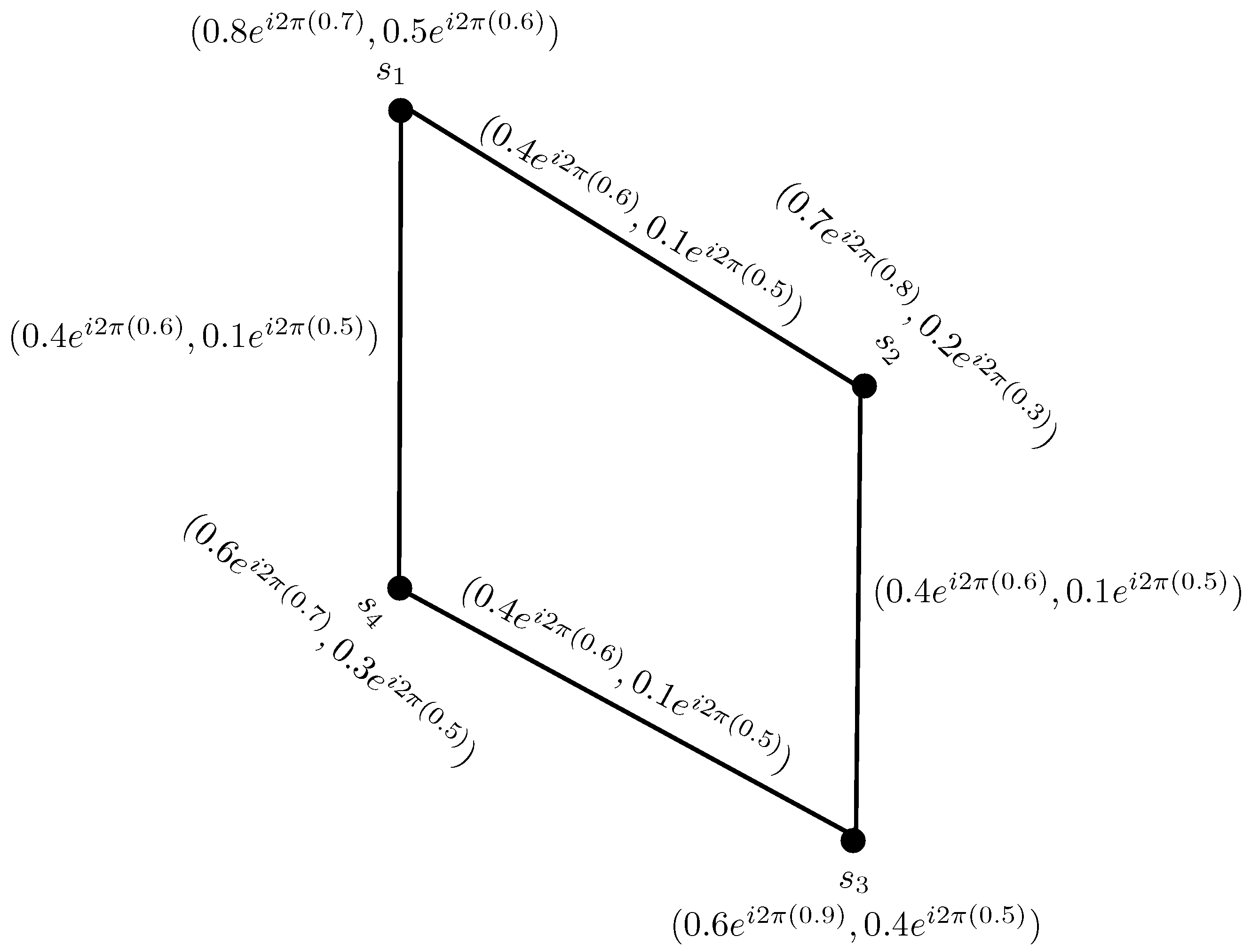
3. Edge Regularity of a Graph in Complex Pythagorean Fuzzy Circumstances

In this section, we propose the concepts of edge regular and totally edge regular complex Pythagorean fuzzy graphs and discuss their properties in detail. Further, these results are elaborated with examples.

Definition 20.

Let $\mathcal{G}=(\mathcal{C},\mathcal{D})$ be a CPFG. The degree of an edge $r_i{r}_j\in D$ is defined as ${\mathrm{d}}_{\mathcal{G}}\left(r_i{r}_j\right)=({\mathrm{d}}_{\mu e^{i\alpha }}\left(r_i{r}_j\right),{\mathrm{d}}_{\nu e^{i\beta }}\left(r_i{r}_j\right)),$ where

$$\begin{array}{ccc}\hfill {\mathrm{d}}_{\mu e^{i\alpha }}\left(r_i{r}_j\right)& =& {\mathrm{d}}_{\mu e^{i\alpha }}\left(r_i\right)+{\mathrm{d}}_{\mu e^{i\alpha }}\left(r_j\right)-2{\mu }_{\mathcal{D}}\left(r_i{r}_j\right)e^{2i{\alpha }_{\mathcal{D}}\left(r_i{r}_j\right)}\hfill \\ & & ={\displaystyle \sum _{\begin{array}{c}{r}_i{r}_k\in D\\ k\ne j\end{array}}}{\mu }_{\mathcal{D}}\left(r_i{r}_k\right)e^{i{\displaystyle \sum _{\begin{array}{c}{r}_i{r}_k\in D\\ k\ne j\end{array}}}{\alpha }_{\mathcal{D}}\left(r_i{r}_k\right)}+{\displaystyle \sum _{\begin{array}{c}{r}_j{r}_k\in D\\ k\ne i\end{array}}}{\mu }_{\mathcal{D}}\left(r_j{r}_k\right)e^{i{\displaystyle \sum _{\begin{array}{c}{r}_j{r}_k\in D\\ k\ne i\end{array}}}{\alpha }_{\mathcal{D}}\left(r_j{r}_k\right)},\hfill \\ \hfill {\mathrm{d}}_{\nu e^{i\beta }}\left(r_i{r}_j\right)& =& {\mathrm{d}}_{\nu e^{i\beta }}\left(r_i\right)+{\mathrm{d}}_{\nu e^{i\beta }}\left(r_j\right)-2{\nu }_{\mathcal{D}}\left(r_i{r}_j\right)e^{2i{\beta }_{\mathcal{D}}\left(r_i{r}_j\right)}\hfill \\ & & ={\displaystyle \sum _{\begin{array}{c}{r}_i{r}_k\in D\\ k\ne j\end{array}}}{\nu }_{\mathcal{D}}\left(r_i{r}_k\right)e^{i{\displaystyle \sum _{\begin{array}{c}{r}_i{r}_k\in D\\ k\ne j\end{array}}}{\beta }_{\mathcal{D}}\left(r_i{r}_k\right)}+{\displaystyle \sum _{\begin{array}{c}{r}_j{r}_k\in D\\ k\ne i\end{array}}}{\nu }_{\mathcal{D}}\left(r_j{r}_k\right)e^{i{\displaystyle \sum _{\begin{array}{c}{r}_j{r}_k\in D\\ k\ne i\end{array}}}{\beta }_{\mathcal{D}}\left(r_j{r}_k\right)}.\hfill \end{array}$$

Definition 21.

The minimum and the maximum edge degree of a CPFG $\mathcal{G}$ is ${\delta }_D\left(\mathcal{G}\right)=({\delta }_{\mu }\left(\mathcal{G}\right),{\delta }_{\nu }\left(\mathcal{G}\right))$ and ${\Delta }_D\left(\mathcal{G}\right)=({\Delta }_{\mu }\left(\mathcal{G}\right),{\Delta }_{\nu }\left(\mathcal{G}\right))$, respectively, where

$$\begin{array}{ccc}\hfill {\delta }_{\mu }\left(\mathcal{G}\right)& =& min\left\{d_{\mu e^{i\alpha }}\left(r_i{r}_j\right)\right|r_i{r}_j\in D\},{\delta }_{\nu }\left(\mathcal{G}\right)=max\left\{d_{\nu e^{i\beta }}\left(r_i{r}_j\right)\right|r_i{r}_j\in D\},\hfill \\ \hfill {\Delta }_{\mu }\left(\mathcal{G}\right)& =& max\left\{d_{\mu e^{i\alpha }}\left(r_i{r}_j\right)\right|r_i{r}_j\in D\},{\Delta }_{\nu }\left(\mathcal{G}\right)=min\left\{d_{\nu e^{i\beta }}\left(r_i{r}_j\right)\right|r_i{r}_j\in D\}.\hfill \end{array}$$

Definition 22.

A CPFG $\mathcal{G}$ on G is called an edge regular, if its each edge has the same degree. If each edge has degree $(s_1,s_2)$, i.e., ${\mathrm{d}}_{\mathcal{G}}\left(r_i{r}_j\right)=(s_1,s_2)$ for all $r_i{r}_j\in D$, where

$$\begin{array}{ccc}\hfill {\mathrm{d}}_{\mu e^{i\alpha }}\left(r_i{r}_j\right)& =& {\displaystyle \sum _{\begin{array}{c}{r}_i{r}_k\in D\\ k\ne j\end{array}}}{\mu }_{\mathcal{D}}\left(r_i{r}_k\right)e^{i{\displaystyle \sum _{\begin{array}{c}{r}_i{r}_k\in D\\ k\ne j\end{array}}}{\alpha }_{\mathcal{D}}\left(r_i{r}_k\right)}+{\displaystyle \sum _{\begin{array}{c}{r}_j{r}_k\in D\\ k\ne i\end{array}}}{\mu }_{\mathcal{D}}\left(r_j{r}_k\right)e^{i{\displaystyle \sum _{\begin{array}{c}{r}_j{r}_k\in D\\ k\ne i\end{array}}}{\alpha }_{\mathcal{D}}\left(r_j{r}_k\right)}=s_1,\hfill \\ \hfill {\mathrm{d}}_{\nu e^{i\beta }}\left(r_i{r}_j\right)& =& {\displaystyle \sum _{\begin{array}{c}{r}_i{r}_k\in D\\ k\ne j\end{array}}}{\nu }_{\mathcal{D}}\left(r_i{r}_k\right)e^{i{\displaystyle \sum _{\begin{array}{c}{r}_i{r}_k\in D\\ k\ne j\end{array}}}{\beta }_{\mathcal{D}}\left(r_i{r}_k\right)}+{\displaystyle \sum _{\begin{array}{c}{r}_j{r}_k\in D\\ k\ne i\end{array}}}{\nu }_{\mathcal{D}}\left(r_j{r}_k\right)e^{i{\displaystyle \sum _{\begin{array}{c}{r}_j{r}_k\in D\\ k\ne i\end{array}}}{\beta }_{\mathcal{D}}\left(r_j{r}_k\right)}=s_2.\hfill \end{array}$$

$\mathcal{G}$ is called edge regular of degree $(s_1,s_2)$ or $(s_1,s_2)$-edge regular.

Example 8.

Consider a CPFG $\mathcal{G}=(\mathcal{C},\mathcal{D})$ on $C=\{s_1,s_2,s_3,s_4\}$, as in Figure 9, defined by:

$$\begin{array}{ccc}\hfill \mathcal{C}& =& 〈\left(\frac{s_1}{0.6e^{i2\pi \left(0.7\right)}},\frac{s_2}{0.4e^{i2\pi \left(0.5\right)}},\frac{s_3}{0.4e^{i2\pi \left(0.6\right)}},\frac{s_4}{0.7e^{i2\pi \left(0.8\right)}}\right),\left(\frac{s_1}{0.7e^{i2\pi \left(0.6\right)}},\frac{s_2}{0.8e^{i2\pi \left(0.8\right)}},\frac{s_3}{0.9e^{i2\pi \left(0.4\right)}},\frac{s_4}{0.5e^{i2\pi \left(0.5\right)}}\right)〉,\hfill \\ \hfill \mathcal{D}& =& 〈\left(\frac{s_1{s}_2}{0.2e^{i2\pi \left(0.3\right)}},\frac{s_2{s}_3}{0.1e^{i2\pi \left(0.2\right)}},\frac{s_3{s}_4}{0.3e^{i2\pi \left(0.4\right)}},\frac{s_1{s}_4}{0.4e^{i2\pi \left(0.5\right)}}\frac{s_1{s}_3}{0.4e^{i2\pi \left(0.5\right)}},\frac{s_2{s}_4}{0.1e^{i2\pi \left(0.2\right)}}\right),\hfill \\ & & \left(\frac{s_1{s}_2}{0.7e^{i2\pi \left(0.7\right)}},\frac{s_2{s}_3}{0.9e^{i2\pi \left(0.6\right)}},\frac{s_3{s}_4}{0.8e^{i2\pi \left(0.5\right)}},\frac{s_1{s}_4}{0.6e^{i2\pi \left(0.6\right)}},\frac{s_1{s}_3}{0.9e^{i2\pi \left(0.4\right)}},\frac{s_2{s}_4}{0.6e^{i2\pi \left(0.8\right)}}\right)〉.\hfill \end{array}$$

Clearly, ${\mathrm{d}}_{\mathcal{G}}\left(s_1{s}_2\right)={\mathrm{d}}_{\mathcal{G}}\left(s_2{s}_3\right)={\mathrm{d}}_{\mathcal{G}}\left(s_3{s}_4\right)={\mathrm{d}}_{\mathcal{G}}\left(s_4{s}_1\right)={\mathrm{d}}_{\mathcal{G}}\left(s_1{s}_3\right)={\mathrm{d}}_{\mathcal{G}}\left(s_2{s}_4\right)=(1.0e^{i2\pi \left(1.4\right)},3.0e^{i2\pi \left(2.4\right)})$. So, $\mathcal{G}$ is $(1.0e^{i2\pi \left(1.4\right)},3.0e^{i2\pi \left(2.4\right)})$-edge regular CPFG.

Theorem 6.

Let $\mathcal{G}=(\mathcal{C},\mathcal{D})$ be a CPFG on a cycle graph G. Then

$${\displaystyle \sum _{r_i\in C}}{\mathrm{d}}_{\mathcal{G}}\left(r_i\right)={\displaystyle \sum _{r_i{r}_j\in D}}{\mathrm{d}}_{\mathcal{G}}\left(r_i{r}_j\right)$$

Proof. 

Let $\mathcal{G}=(\mathcal{C},\mathcal{D})$ be a CPFG and let G be a cycle $r_1{r}_2{r}_3\dots r_n{r}_1.$ Then

$$\begin{array}{c}\hfill {\displaystyle \sum _{i=1}^n}{\mathrm{d}}_{\mathcal{G}}\left(r_i{r}_{i+1}\right)=\left({\displaystyle \sum _{i=1}^n}{\mathrm{d}}_{\mu e^{i\alpha }}\left(r_i{r}_{i+1}\right),{\displaystyle \sum _{i=1}^n}{\mathrm{d}}_{\nu e^{i\beta }}\left(r_i{r}_{i+1}\right)\right).\end{array}$$

Consider

$$\begin{array}{ccc}\hfill {\displaystyle \sum _{i=1}^n}{\mathrm{d}}_{\mu e^{i\alpha }}\left(r_i{r}_{i+1}\right)& =& {\mathrm{d}}_{\mu e^{i\alpha }}\left(r_1{r}_2\right)+{\mathrm{d}}_{\mu e^{i\alpha }}\left(r_2{r}_3\right)+\dots +{\mathrm{d}}_{\mu e^{i\alpha }}\left(r_n{r}_1\right),where{r}_{n+1}=r_1\hfill \\ & =& {\mathrm{d}}_{\mu e^{i\alpha }}\left(r_1\right)+{\mathrm{d}}_{\mu e^{i\alpha }}\left(r_2\right)-2{\mu }_{\mathcal{D}}\left(r_1{r}_2\right)e^{2i{\alpha }_{\mathcal{D}}\left(r_1{r}_2\right)}+{\mathrm{d}}_{\mu e^{i\alpha }}\left(r_2\right)+{\mathrm{d}}_{\mu e^{i\alpha }}\left(r_3\right)-2{\mu }_{\mathcal{D}}\left(r_2{r}_3\right)e^{2i{\alpha }_{\mathcal{D}}\left(r_2{r}_3\right)}\hfill \\ & & +\dots +{\mathrm{d}}_{\mu e^{i\alpha }}\left(r_n\right)+{\mathrm{d}}_{\mu e^{i\alpha }}\left(r_1\right)-2{\mu }_{\mathcal{D}}\left(r_n{r}_1\right)e^{2{\alpha }_{\mathcal{D}}\left(r_n{r}_1\right)}\hfill \\ & =& 2{\mathrm{d}}_{\mu e^{2i\alpha }}\left(r_1\right)+2{\mathrm{d}}_{\mu e^{2i\alpha }}\left(r_2\right)+\dots +2{\mathrm{d}}_{\mu e^{2i\alpha }}\left(r_n\right)\hfill \\ & & -2\left({\mu }_{\mathcal{D}}{\left(r_1{r}_2\right)}^{2i{\alpha }_{\mathcal{D}}\left(r_1{r}_2\right)}+{\mu }_{\mathcal{D}}\left(r_2{u}_3\right)e^{2i{\alpha }_{\mathcal{D}}\left(r_2{u}_3\right)}+\dots +{\mu }_{\mathcal{D}}\left(r_n{r}_1\right)e^{2i{\alpha }_{\mathcal{D}}\left(r_n{r}_1\right)}\right)\hfill \\ & =& 2{\displaystyle \sum _{r_i\in C}}{\mathrm{d}}_{\mu e^{i\alpha }}\left(r_i\right)-2{\displaystyle \sum _{i=1}^n}{\mu }_{\mathcal{D}}\left(r_i{r}_{i+1}\right)e^{2i{\displaystyle \sum _{i=1}^n}{\alpha }_{\mathcal{D}}\left(r_i{r}_{i+1}\right)}\hfill \\ & =& {\displaystyle \sum _{r_i\in C}}{\mathrm{d}}_{\mu e^{i\alpha }}\left(r_i\right)+{\displaystyle \sum _{r_i\in C}}{\mathrm{d}}_{\mu e^{i\alpha }}\left(r_i\right)-2{\displaystyle \sum _{i=1}^n}{\mu }_{\mathcal{D}}\left(r_i{r}_{i+1}\right)e^{2i{\displaystyle \sum _{i=1}^n}{\alpha }_{\mathcal{D}}\left(r_i{r}_{i+1}\right)}\hfill \\ & =& {\displaystyle \sum _{r_i\in C}}{\mathrm{d}}_{\mu e^{i\alpha }}\left(r_i\right)+2{\displaystyle \sum _{i=1}^n}{\mu }_{\mathcal{D}}\left(r_i{r}_{i+1}\right)e^{2i{\displaystyle \sum _{i=1}^n}{\alpha }_{\mathcal{D}}\left(r_i{r}_{i+1}\right)}-2{\displaystyle \sum _{i=1}^n}{\mu }_{\mathcal{D}}\left(r_i{r}_{i+1}\right)e^{2i{\displaystyle \sum _{i=1}^n}{\alpha }_{\mathcal{D}}\left(r_i{r}_{i+1}\right)}\hfill \\ & =& {\displaystyle \sum _{r_i\in C}}{\mathrm{d}}_{\mu e^{i\alpha }}\left(r_i\right).\hfill \end{array}$$

Similarly, ${\displaystyle \sum _{i=1}^n}{\mathrm{d}}_{\nu e^{i\beta }}\left(r_i{r}_{i+1}\right)={\displaystyle \sum _{r_i\in C}}{\mathrm{d}}_{\nu e^{i\beta }}\left(r_i\right)$. Hence ${\displaystyle \sum _{r_i\in C}}{\mathrm{d}}_{\mathcal{G}}\left(r_i\right)={\displaystyle \sum _{r_i{r}_j\in D}}{\mathrm{d}}_{\mathcal{G}}\left(r_i{r}_j\right).$ □

Theorem 7.

Let $\mathcal{G}=(\mathcal{C},\mathcal{D})$ be a CPFG on a regular graph G. Then

$$\begin{array}{ccc}\hfill {\displaystyle \sum _{r_i{r}_j\in D}}{\mathrm{d}}_{\mathcal{G}}\left(r_i{r}_j\right)& =& \left({\displaystyle \sum _{r_i{r}_j\in D}}{\mathrm{d}}_G\left(r_i{r}_j\right){\mu }_{\mathcal{D}}\left(r_i{r}_j\right)e^{i{\alpha }_{\mathcal{D}}\left(r_i{r}_j\right)},{\displaystyle \sum _{r_i{r}_j\in D}}{\mathrm{d}}_G\left(r_i{r}_j\right){\nu }_{\mathcal{D}}\left(r_i{r}_j\right)e^{i{\beta }_{\mathcal{D}}\left(r_i{r}_j\right)}\right),\hfill \end{array}$$

where ${\mathrm{d}}_G\left(r_i{r}_j\right)={\mathrm{d}}_G\left(r_i\right)+{\mathrm{d}}_G\left(r_j\right)-2$ for all $r_i{r}_j\in D$.

Proposition 2.

Let $\mathcal{G}=(\mathcal{C},\mathcal{D})$ be a CPFG on a l-regular graph G. Then

$$\begin{array}{ccc}\hfill {\displaystyle \sum _{r_i{r}_j\in D}}{\mathrm{d}}_{\mathcal{G}}\left(r_i{r}_j\right)& =& \left((l-1){\displaystyle \sum _{r_i\in C}}{\mathrm{d}}_{\mu e^{i\alpha }}\left(r_i\right),(l-1){\displaystyle \sum _{r_i\in C}}{\mathrm{d}}_{\nu e^{i\beta }}\left(r_i\right)\right).\hfill \end{array}$$

Proof. 

Suppose that $\mathcal{G}$ is a CPFG on a l-regular graph G. Utilizing Theorem 7, we get

$$\begin{array}{ccc}\hfill {\displaystyle \sum _{r_i{r}_j\in D}}{\mathrm{d}}_{\mathcal{G}}\left(r_i{r}_j\right)& =& \left({\displaystyle \sum _{r_i{r}_j\in D}}{\mathrm{d}}_G\left(r_i{r}_j\right){\mu }_{\mathcal{D}}\left(r_i{r}_j\right)e^{i{\alpha }_{\mathcal{D}}\left(r_i{r}_j\right)},{\displaystyle \sum _{r_i{r}_j\in D}}{\mathrm{d}}_G\left(r_i{r}_j\right){\nu }_{\mathcal{D}}\left(r_i{r}_j\right)e^{i{\beta }_{\mathcal{D}}\left(r_i{r}_j\right)}\right)\hfill \\ & =& \left({\displaystyle \sum _{r_i{r}_j\in D}}({\mathrm{d}}_G\left(r_i\right)+{\mathrm{d}}_G\left(r_j\right)-2){\mu }_{\mathcal{D}}\left(r_i{r}_j\right)e^{i{\alpha }_{\mathcal{D}}\left(r_i{r}_j\right)},{\displaystyle \sum _{r_i{r}_j\in D}}({\mathrm{d}}_G\left(r_i\right)+{\mathrm{d}}_G\left(r_j\right)-2){\nu }_{\mathcal{D}}\left(r_i{r}_j\right)e^{i{\beta }_{\mathcal{D}}\left(r_i{r}_j\right)}\right).\hfill \end{array}$$

Since G is a l-regular graph, ${\mathrm{d}}_G\left(r_i\right)=l,$ for all $r_i\in C$, so

$$\begin{array}{ccc}\hfill {\displaystyle \sum _{r_i{r}_j\in D}}{\mathrm{d}}_{\mathcal{G}}\left(r_i{r}_j\right)& =& \left(2(l-1){\displaystyle \sum _{r_i{r}_j\in D}}{\mu }_{\mathcal{D}}\left(r_i{r}_j\right)e^{i{\displaystyle \sum _{r_i{r}_j\in D}}{\alpha }_{\mathcal{D}}\left(r_i{r}_j\right)},2(l-1){\displaystyle \sum _{r_i{r}_j\in D}}{\nu }_{\mathcal{D}}\left(r_i{r}_j\right)e^{i{\displaystyle \sum _{r_i{r}_j\in D}}{\beta }_{\mathcal{D}}\left(r_i{r}_j\right)}\right),\hfill \\ & =& \left((l-1){\displaystyle \sum _{r_i\in C}}{\mathrm{d}}_{\mu e^{i\alpha }}\left(r_i\right),(l-1){\displaystyle \sum _{r_i\in C}}{\mathrm{d}}_{\nu e^{i\beta }}\left(r_i\right)\right).\hfill \end{array}$$

 □

Theorem 8.

Let $\mathcal{G}=(\mathcal{C},\mathcal{D})$ be a CPFG on a graph G. If $({\mu }_{\mathcal{D}}{e}^{i{\alpha }_{\mathcal{D}}},{\nu }_{\mathcal{D}}{e}^{i{\beta }_{\mathcal{D}}})$ is a constant function, then $\mathcal{G}$ is an edge regular CPFG if and only if G is an edge regular.

Proof. 

Suppose that $({\mu }_{\mathcal{D}}{e}^{i{\alpha }_{\mathcal{D}}},{\nu }_{\mathcal{D}}{e}^{i{\beta }_{\mathcal{D}}})$ is a constant function, ${\mu }_{\mathcal{D}}\left(r_i{r}_j\right)e^{i{\alpha }_{\mathcal{D}}\left(r_i{r}_j\right)}=c_1{e}^{i2\pi \left(c_1^{{}^{\prime }}\right)}$ and ${\nu }_{\mathcal{D}}\left(r_i{r}_j\right)e^{i{\beta }_{\mathcal{D}}\left(r_i{r}_j\right)}=c_2{e}^{i2\pi \left(c_2^{{}^{\prime }}\right)}$ for all $r_i{r}_j\in D$, where $c_1{e}^{i2\pi \left(c_1^{{}^{\prime }}\right)}$ and $c_2{e}^{i2\pi \left(c_2^{{}^{\prime }}\right)}$ are constants. Assume that $\mathcal{G}$ is an edge regular CPFG. We show that G is an edge regular. On the contrary, suppose that G is an edge irregular, i.e., ${\mathrm{d}}_G\left(r_i{r}_j\right)\ne {\mathrm{d}}_G\left(r_l{r}_m\right)$ for at least on pair of $r_i{r}_j,r_l{r}_m\in D$.

From the definition of edge degree of a CPFG,

$${\mathrm{d}}_{\mathcal{G}}\left(r_i{r}_j\right)=({\mathrm{d}}_{\mu e^{i\alpha }}\left(r_i{r}_j\right),{\mathrm{d}}_{\nu e^{i\beta }}\left(r_i{r}_j\right)),$$

where

$$\begin{array}{ccc}\hfill {\mathrm{d}}_{\mu e^{i\alpha }}\left(r_i{r}_j\right)& =& {\displaystyle \sum _{\begin{array}{c}{r}_i{r}_k\in D\\ k\ne j\end{array}}}{\mu }_{\mathcal{D}}\left(r_i{r}_k\right)e^{i{\displaystyle \sum _{\begin{array}{c}{r}_i{r}_k\in D\\ k\ne j\end{array}}}{\alpha }_{\mathcal{D}}\left(r_i{r}_k\right)}+{\displaystyle \sum _{\begin{array}{c}{r}_j{r}_k\in D\\ k\ne i\end{array}}}{\mu }_{\mathcal{D}}\left(r_j{r}_k\right)e^{i{\displaystyle \sum _{\begin{array}{c}{r}_j{r}_k\in D\\ k\ne i\end{array}}}{\alpha }_{\mathcal{D}}\left(r_j{r}_k\right)}\hfill \\ & =& {\displaystyle \sum _{\begin{array}{c}{r}_i{r}_k\in D\\ k\ne j\end{array}}}{c}_1{e}^{i2\pi \left({\displaystyle \sum _{\begin{array}{c}{r}_i{r}_k\in D\\ k\ne j\end{array}}}{c}_1^{{}^{\prime }}\right)}+{\displaystyle \sum _{\begin{array}{c}{r}_j{r}_k\in D\\ k\ne i\end{array}}}{c}_1{e}^{i2\pi \left({\displaystyle \sum _{\begin{array}{c}{r}_j{r}_k\in D\\ k\ne i\end{array}}}{c}_1^{{}^{\prime }}\right)}\hfill \\ & =& c_1{e}^{i2\pi \left(c_1^{{}^{\prime }}\right)}({\mathrm{d}}_G\left(r_i\right)-1)+c_1{e}^{i2\pi \left(c_1^{{}^{\prime }}\right)}({\mathrm{d}}_G\left(r_j\right)-1)\hfill \\ & =& c_1{e}^{i2\pi \left(c_1^{{}^{\prime }}\right)}({\mathrm{d}}_G\left(r_i\right)+{\mathrm{d}}_G\left(r_j\right)-2)\hfill \\ & =& c_1{e}^{i2\pi \left(c_1^{{}^{\prime }}\right)}{\mathrm{d}}_G\left(r_i{r}_j\right)\mathrm{for} \mathrm{all}{r}_i{r}_j\in D.\hfill \end{array}$$

Analogously, we can show that ${\mathrm{d}}_{\nu e^{i\beta }}\left(r_i{r}_j\right)=c_2{e}^{i2\pi \left(c_2^{{}^{\prime }}\right)}{\mathrm{d}}_G\left(r_i{r}_j\right)$ for all $r_i{r}_j\in D.$ Therefore ${\mathrm{d}}_{\mathcal{G}}\left(r_i{r}_j\right)=(c_1{e}^{i2\pi \left(c_1^{{}^{\prime }}\right)}{\mathrm{d}}_G\left(r_i{r}_j\right),c_2{e}^{i2\pi \left(c_2^{{}^{\prime }}\right)}{\mathrm{d}}_G\left(r_i{r}_j\right)),$${\mathrm{d}}_{\mathcal{G}}\left(r_l{r}_m\right)=(c_1{e}^{i2\pi \left(c_1^{{}^{\prime }}\right)}{\mathrm{d}}_G\left(r_l{r}_m\right),c_2{e}^{i2\pi \left(c_2^{{}^{\prime }}\right)}{\mathrm{d}}_G\left(r_l{r}_m\right)).$ Since ${\mathrm{d}}_G\left(r_i{r}_j\right)\ne {\mathrm{d}}_G\left(r_l{r}_m\right)$, so ${\mathrm{d}}_{\mathcal{G}}\left(r_i{r}_j\right)\ne {\mathrm{d}}_{\mathcal{G}}\left(r_l{r}_m\right)$. Thus $\mathcal{G}$ is an edge irregular, a contradiction. Hence G is an edge regular.

Conversely, let G be an edge regular. To show that $\mathcal{G}$ is an edge regular CPFG. Consider $\mathcal{G}$ is an edge irregular CPFG. i.e., ${\mathrm{d}}_{\mathcal{G}}\left(r_i{r}_j\right)\ne {\mathrm{d}}_{\mathcal{G}}\left(r_p{r}_q\right)$ for at least one pair of $r_i{r}_j,r_p{r}_q\in D,$ $({\mathrm{d}}_{\mu e^{i\alpha }}\left(r_i{r}_j\right),{\mathrm{d}}_{\nu e^{i\beta }}\left(r_i{r}_j\right))\ne ({\mathrm{d}}_{\mu e^{i\alpha }}\left(r_p{r}_q\right),{\mathrm{d}}_{\nu e^{i\beta }}\left(r_p{r}_q\right)).$ Now ${\mathrm{d}}_{\mu e^{i\alpha }}\left(r_i{r}_j\right)\ne {\mathrm{d}}_{\mu e^{i\alpha }}\left(r_p{r}_q\right)$ implies ${\displaystyle \sum _{\begin{array}{c}{r}_i{r}_k\in D\\ k\ne j\end{array}}}{\mu }_{\mathcal{D}}\left(r_i{r}_k\right)e^{i{\displaystyle \sum _{\begin{array}{c}{r}_i{r}_k\in D\\ k\ne j\end{array}}}{\alpha }_{\mathcal{D}}\left(r_i{r}_k\right)}+{\displaystyle \sum _{\begin{array}{c}{r}_j{r}_k\in D\\ k\ne i\end{array}}}{\mu }_{\mathcal{D}}\left(r_j{r}_k\right)e^{i{\displaystyle \sum _{\begin{array}{c}{r}_j{r}_k\in D\\ k\ne i\end{array}}}{\alpha }_{\mathcal{D}}\left(r_j{r}_k\right)}\ne {\displaystyle \sum _{\begin{array}{c}{r}_p{r}_s\in D\\ s\ne q\end{array}}}{\mu }_{\mathcal{D}}\left(r_p{r}_s\right)e^{i{\displaystyle \sum _{\begin{array}{c}{r}_p{r}_s\in D\\ s\ne q\end{array}}}{\beta }_{\mathcal{D}}\left(r_p{r}_s\right)}+{\displaystyle \sum _{\begin{array}{c}{r}_s{r}_q\in D\\ s\ne p\end{array}}}{\mu }_{\mathcal{D}}\left(r_s{r}_q\right)e^{i{\displaystyle \sum _{\begin{array}{c}{r}_s{r}_q\in D\\ s\ne p\end{array}}}{\beta }_{\mathcal{D}}\left(r_s{r}_q\right)}$, since ${\mu }_{\mathcal{D}}{e}^{i{\alpha }_{\mathcal{D}}}$ is a constant, so ${\mathrm{d}}_G\left(r_i{r}_j\right)\ne {\mathrm{d}}_G\left(r_p{r}_q\right)$, a contradiction. Therefore $\mathcal{G}$ is an edge regular CPFG. □

Theorem 9.

Let $\mathcal{G}=(\mathcal{C},\mathcal{D})$ be a regular CPFG. Then $\mathcal{G}$ is an edge regular CPFG if and only if $({\mu }_{\mathcal{D}}{e}^{i{\alpha }_{\mathcal{D}}},{\nu }_{\mathcal{D}}{e}^{i{\beta }_{\mathcal{D}}})$ is a constant function.

Proof. 

Let $\mathcal{G}$ be a $(r_1,r_2)$-regular CPFG i.e., ${\mathrm{d}}_{\mathcal{G}}\left(r_i\right)=(r_1,r_2)$ for all $r_i\in C$. Suppose that $({\mu }_{\mathcal{D}}{e}^{i{\alpha }_{\mathcal{D}}},{\nu }_{\mathcal{D}}{e}^{i{\beta }_{\mathcal{D}}})$ is a constant function. Then ${\mu }_{\mathcal{D}}\left(r_i{r}_j\right)e^{i{\alpha }_{\mathcal{D}}\left(r_i{r}_j\right)}=c_1{e}^{i2\pi \left(c_1^{{}^{\prime }}\right)}$ and ${\nu }_{\mathcal{D}}\left(r_i{r}_j\right)e^{{\beta }_{\mathcal{D}}\left(r_i{r}_j\right)}=c_2{e}^{i2\pi \left(c_2^{{}^{\prime }}\right)}$ for all $r_i{r}_j\in D$, where $c_1{e}^{i2\pi \left(c_1^{{}^{\prime }}\right)}$ and $c_2{e}^{i2\pi \left(c_2^{{}^{\prime }}\right)}$ are constants. By definition of edge degree of a CPFG,

$${\mathrm{d}}_{\mathcal{G}}\left(r_i{r}_j\right)=({\mathrm{d}}_{\mu e^{i\alpha }}\left(r_i{r}_j\right),{\mathrm{d}}_{\nu e^{i\beta }}\left(r_i{r}_j\right)),$$

where

$$\begin{array}{ccc}\hfill {\mathrm{d}}_{\mu e^{i\alpha }}\left(r_i{r}_j\right)& =& {\mathrm{d}}_{\mu e^{i\alpha }}\left(r_i\right)+{\mathrm{d}}_{\mu e^{i\alpha }}\left(r_j\right)-2{\mu }_{\mathcal{D}}\left(r_i{r}_j\right)e^{2i{\alpha }_{\mathcal{D}}\left(r_i{r}_j\right)}\hfill \\ & =& r_1+r_1-2c_1{e}^{i2\pi \left(c_1^{{}^{\prime }}\right)}\hfill \\ & =& 2(r_1-c_1{e}^{i2\pi \left(c_1^{{}^{\prime }}\right)})\mathrm{for} \mathrm{all}{r}_i{r}_j\in D.\hfill \end{array}$$

Similarly, ${\mathrm{d}}_{\nu e^{i\beta }}\left(r_i{r}_j\right)=2(r_2-c_2{e}^{i2\pi \left(c_2^{{}^{\prime }}\right)})$ for all $r_i{r}_j\in D$. Hence $\mathcal{G}$ is an edge regular CPFG.

Conversely, assume that $\mathcal{G}$ is an edge regular CPFG, i.e., ${\mathrm{d}}_{\mathcal{G}}\left(r_i{r}_j\right)=(s_1,s_2)$ for all $r_i{r}_j\in D.$ We show that $({\mu }_{\mathcal{D}}{e}^{i{\alpha }_{\mathcal{D}}},{\nu }_{\mathcal{D}}{e}^{i{\beta }_{\mathcal{D}}})$ is a constant function. Since ${\mathrm{d}}_{\mathcal{G}}\left(r_i{r}_j\right)=({\mathrm{d}}_{\mu e^{i\alpha }}\left(r_i{r}_j\right),{\mathrm{d}}_{\nu e^{i\beta }}\left(r_i{r}_j\right))$, where

$$\begin{array}{ccc}\hfill {\mathrm{d}}_{\mu e^{i\alpha }}\left(r_i{r}_j\right)& =& {\mathrm{d}}_{\mu e^{i\alpha }}\left(r_i\right)+{\mathrm{d}}_{\mu e^{i\alpha }}\left(r_j\right)-2{\mu }_{\mathcal{D}}\left(r_i{r}_j\right)e^{2i{\alpha }_{\mathcal{D}}\left(r_i{r}_j\right)}\hfill \\ \hfill s_1& =& r_1+r_1-2{\mu }_{\mathcal{D}}\left(r_i{r}_j\right)e^{2i{\alpha }_{\mathcal{D}}\left(r_i{r}_j\right)}\hfill \\ \hfill {\mu }_{\mathcal{D}}\left(r_i{r}_j\right)e^{2i{\alpha }_{\mathcal{D}}\left(r_i{r}_j\right)}& =& \frac{(2r_1-s_1)}{2}\mathrm{for} \mathrm{all}{r}_i{r}_j\in D.\hfill \end{array}$$

Similarly, ${\nu }_{\mathcal{D}}\left(r_i{r}_j\right)e^{2i{\beta }_{\mathcal{D}}\left(r_i{r}_j\right)}=\frac{(2r_2-s_2)}{2}$ for all $r_i{r}_j\in D$. Hence $({\mu }_{\mathcal{D}}{e}^{i{\alpha }_{\mathcal{D}}},{\nu }_{\mathcal{D}}{e}^{i{\beta }_{\mathcal{D}}})$ is a constant function. □

Definition 23.

The total degree of an edge $r_i{r}_j\in D$ in a CPFG $\mathcal{G}=(\mathcal{C},\mathcal{D})$ is defined as $t{\mathrm{d}}_{\mathcal{G}}\left(r_i{r}_j\right)=(t{\mathrm{d}}_{\mu e^{i\alpha }}\left(r_i{r}_j\right),t{\mathrm{d}}_{\nu e^{i\beta }}\left(r_i{r}_j\right)),$ where

$$\begin{array}{ccc}\hfill t{\mathrm{d}}_{\mu e^{i\alpha }}\left(r_i{r}_j\right)& =& {\mathrm{d}}_{\mu e^{i\alpha }}\left(r_i\right)+{\mathrm{d}}_{\mu e^{i\alpha }}\left(r_j\right)-{\mu }_{\mathcal{D}}\left(r_i{r}_j\right)e^{i{\alpha }_{\mathcal{D}}\left(r_i{r}_j\right)}\hfill \\ & =& {\displaystyle \sum _{\begin{array}{c}{r}_i{r}_k\in D\\ k\ne j\end{array}}}{\mu }_{\mathcal{D}}\left(r_i{r}_k\right)e^{i{\displaystyle \sum _{\begin{array}{c}{r}_i{r}_k\in D\\ k\ne j\end{array}}}{\alpha }_{\mathcal{D}}\left(r_i{r}_k\right)}+{\displaystyle \sum _{\begin{array}{c}{r}_j{r}_k\in D\\ k\ne i\end{array}}}{\mu }_{\mathcal{D}}\left(r_j{r}_k\right)e^{i{\displaystyle \sum _{\begin{array}{c}{r}_j{r}_k\in D\\ k\ne i\end{array}}}{\alpha }_{\mathcal{D}}\left(r_j{r}_k\right)}+{\mu }_{\mathcal{D}}\left(r_i{r}_j\right)e^{i{\alpha }_{\mathcal{D}}\left(r_i{r}_j\right)},\hfill \\ \hfill t{\mathrm{d}}_{\nu e^{i\beta }}\left(r_i{r}_j\right)& =& {\mathrm{d}}_{\nu e^{i\beta }}\left(r_i\right)+{\mathrm{d}}_{\nu e^{i\beta }}\left(r_j\right)-{\nu }_{\mathcal{D}}\left(r_i{r}_j\right)e^{i{\beta }_{\mathcal{D}}\left(r_i{r}_j\right)}\hfill \\ & =& {\displaystyle \sum _{\begin{array}{c}{r}_i{r}_k\in D\\ k\ne j\end{array}}}{\nu }_{\mathcal{D}}\left(r_i{r}_k\right)e^{i{\displaystyle \sum _{\begin{array}{c}{r}_i{r}_k\in D\\ k\ne j\end{array}}}{\beta }_{\mathcal{D}}\left(r_i{r}_k\right)}+{\displaystyle \sum _{\begin{array}{c}{r}_j{r}_k\in D\\ k\ne i\end{array}}}{\nu }_{\mathcal{D}}\left(r_j{r}_k\right)e^{i{\displaystyle \sum _{\begin{array}{c}{r}_j{r}_k\in D\\ k\ne i\end{array}}}{\beta }_{\mathcal{D}}\left(r_j{r}_k\right)}+{\nu }_{\mathcal{D}}\left(r_i{r}_j\right)e^{i{\beta }_{\mathcal{D}}\left(r_i{r}_j\right)}.\hfill \end{array}$$

Definition 24.

A CPFG $\mathcal{G}$ on G is called a totally edge regular, if its each edge has the same total degree. If each edge has total degree $({\mathcal{S}}_1,{\mathcal{S}}_2)$, i.e., ${\mathrm{d}}_{\mathcal{G}}\left(r_i{r}_j\right)=({\mathcal{S}}_1,{\mathcal{S}}_2)$ for all $r_i{r}_j\in D$, where

$$\begin{array}{ccc}\hfill \mathrm{t}{\mathrm{d}}_{\mu e^{i\alpha }}\left(r_i{r}_j\right)& =& {\displaystyle \sum _{\begin{array}{c}{r}_i{r}_k\in D\\ k\ne j\end{array}}}{\mu }_{\mathcal{D}}\left(r_i{r}_k\right)e^{i{\displaystyle \sum _{\begin{array}{c}{r}_i{r}_k\in D\\ k\ne j\end{array}}}{\alpha }_{\mathcal{D}}\left(r_i{r}_k\right)}+{\displaystyle \sum _{\begin{array}{c}{r}_j{r}_k\in D\\ k\ne i\end{array}}}{\mu }_{\mathcal{D}}\left(r_j{r}_k\right)e^{i{\displaystyle \sum _{\begin{array}{c}{r}_j{r}_k\in D\\ k\ne i\end{array}}}{\alpha }_{\mathcal{D}}\left(r_j{r}_k\right)}+{\mu }_{\mathcal{D}}\left(r_i{r}_j\right)e^{i{\alpha }_{\mathcal{D}}\left(r_i{r}_j\right)}={\mathcal{S}}_1,\hfill \\ \hfill \mathrm{t}{\mathrm{d}}_{\nu e^{i\beta }}\left(r_i{r}_j\right)& =& {\displaystyle \sum _{\begin{array}{c}{r}_i{r}_k\in D\\ k\ne j\end{array}}}{\nu }_{\mathcal{D}}\left(r_i{r}_k\right)e^{i{\displaystyle \sum _{\begin{array}{c}{r}_i{r}_k\in D\\ k\ne j\end{array}}}{\beta }_{\mathcal{D}}\left(r_i{r}_k\right)}+{\displaystyle \sum _{\begin{array}{c}{r}_j{r}_k\in D\\ k\ne i\end{array}}}{\nu }_{\mathcal{D}}\left(r_j{r}_k\right)e^{i{\displaystyle \sum _{\begin{array}{c}{r}_j{r}_k\in D\\ k\ne i\end{array}}}{\beta }_{\mathcal{D}}\left(r_j{r}_k\right)}+{\nu }_{\mathcal{D}}\left(r_i{r}_j\right)e^{i{\beta }_{\mathcal{D}}\left(r_i{r}_j\right)}={\mathcal{S}}_2.\hfill \end{array}$$

$\mathcal{G}$ is called totally edge regular of degree $({\mathcal{S}}_1,{\mathcal{S}}_2)$ or $({\mathcal{S}}_1,{\mathcal{S}}_2)$-totally edge regular.

Example 9.

Consider a CPFG $\mathcal{G}=(\mathcal{C},\mathcal{D})$ on $C=\{s_1,s_2,s_3,s_4\}$, as in Figure 10, defined by:

$$\begin{array}{ccc}\hfill \mathcal{C}& =& 〈\left(\frac{s_1}{0.8e^{i2\pi \left(0.7\right)}},\frac{s_2}{0.7e^{i2\pi \left(0.8\right)}},\frac{s_3}{0.6e^{i2\pi \left(0.9\right)}},\frac{s_4}{0.6e^{i2\pi \left(0.7\right)}}\right),\left(\frac{s_1}{0.5e^{i2\pi \left(0.6\right)}},\frac{s_2}{0.2e^{i2\pi \left(0.3\right)}},\frac{s_3}{0.4e^{i2\pi \left(0.5\right)}},\frac{s_4}{0.3e^{i2\pi \left(0.5\right)}}\right)〉,\hfill \\ \hfill \mathcal{D}& =& 〈\left(\frac{s_1{s}_2}{0.4e^{i2\pi \left(0.6\right)}},\frac{s_2{s}_3}{0.4e^{i2\pi \left(0.6\right)}},\frac{s_3{s}_4}{0.4e^{i2\pi \left(0.6\right)}},\frac{s_4{s}_1}{0.4e^{i2\pi \left(0.6\right)}}\right),\left(\frac{s_1{s}_2}{0.1e^{i2\pi \left(0.5\right)}},\frac{s_2{s}_3}{0.1e^{i2\pi \left(0.5\right)}},\frac{s_3{s}_4}{0.1e^{i2\pi \left(0.5\right)}},\frac{s_4{s}_1}{0.1e^{i2\pi \left(0.5\right)}}\right)〉.\hfill \end{array}$$

Clearly, $\mathrm{t}{\mathrm{d}}_{\mathcal{G}}\left(s_1{s}_2\right)=\mathrm{t}{\mathrm{d}}_{\mathcal{G}}\left(s_2{s}_3\right)=\mathrm{t}{\mathrm{d}}_{\mathcal{G}}\left(s_3{s}_4\right)=\mathrm{t}{\mathrm{d}}_{\mathcal{G}}\left(s_4{s}_1\right)=(1.2e^{i2\pi \left(1.8\right)},0.3e^{i2\pi \left(1.5\right)})$. So, $\mathcal{G}$ is $(1.2e^{i2\pi \left(1.8\right)},0.3e^{i2\pi \left(1.5\right)})$-totally regular CPFG.

Theorem 10.

Let $\mathcal{G}=(\mathcal{C},\mathcal{D})$ be a CPFG on a regular graph G. Then

$$\begin{array}{ccc}\hfill {\displaystyle \sum _{r_i{r}_j\in D}}t{\mathrm{d}}_{\mathcal{G}}\left(r_i{r}_j\right)& =& \left({\displaystyle \sum _{r_i{r}_j\in D}}{\mathrm{d}}_G\left(r_i{r}_j\right){\mu }_{\mathcal{D}}\left(r_i{r}_j\right)e^{i{\alpha }_{\mathcal{D}}\left(r_i{r}_j\right)}+{\displaystyle \sum _{r_i{r}_j\in D}}{\mu }_{\mathcal{D}}\left(r_i{r}_j\right)e^{i{\displaystyle \sum _{r_i{r}_j\in D}}{\alpha }_{\mathcal{D}}\left(r_i{r}_j\right)},\right.\hfill \\ & & \left.{\displaystyle \sum _{r_i{r}_j\in D}}{\mathrm{d}}_G\left(r_i{r}_j\right){\nu }_{\mathcal{D}}\left(r_i{r}_j\right)e^{i{\beta }_{\mathcal{D}}\left(r_i{r}_j\right)}+{\displaystyle \sum _{r_i{r}_j\in D}}{\nu }_{\mathcal{D}}\left(r_i{r}_j\right)e^{i{\displaystyle \sum _{r_i{r}_j\in D}}{\beta }_{\mathcal{D}}\left(r_i{r}_j\right)}\right).\hfill \end{array}$$

Theorem 11.

Let $\mathcal{G}=(\mathcal{C},\mathcal{D})$ be a CPFG. Then $({\mu }_{\mathcal{D}}{e}^{i{\alpha }_{\mathcal{D}}},{\nu }_{\mathcal{D}}{e}^{i{\beta }_{\mathcal{D}}})$ is a constant function if and only if the statements given below are equivalent:

(i) 

$\mathcal{G}$ is an edge regular CPFG;

(ii) 

$\mathcal{G}$ is a totally edge regular CPFG.

Proof. 

Assume that $({\mu }_{\mathcal{D}}{e}^{i{\alpha }_{\mathcal{D}}},{\nu }_{\mathcal{D}}{e}^{i{\beta }_{\mathcal{D}}})$ is a constant function. Then ${\mu }_{\mathcal{D}}\left(r_i{r}_j\right)e^{i{\alpha }_{\mathcal{D}}\left(r_i{r}_j\right)}=c_1{e}^{i2\pi \left(c_1^{{}^{\prime }}\right)}$ and ${\nu }_{\mathcal{D}}\left(r_i{r}_j\right)e^{i{\beta }_{\mathcal{D}}\left(r_i{r}_j\right)}=c_2{e}^{i2\pi \left(c_2^{{}^{\prime }}\right)}$ for every $r_i{r}_j\in D$, where $c_1{e}^{i2\pi \left(c_1^{{}^{\prime }}\right)}$ and $c_2{e}^{i2\pi \left(c_2^{{}^{\prime }}\right)}$ are constants.

$\left(i\right)\Rightarrow \left(ii\right)$. Suppose that $\mathcal{G}$ is $(s_1,s_2)$-edge regular CPFG. Then ${\mathrm{d}}_{\mathcal{G}}\left(r_i{r}_j\right)=(s_1,s_2)$ for all $r_i{r}_j\in D$.

Consider

$$\begin{array}{c}\left({\mathrm{d}}_{\mu e^{i\alpha }}\left(r_i{r}_j\right)+{\mu }_{\mathcal{D}}\left(r_i{r}_j\right)e^{i{\alpha }_{\mathcal{D}}\left(r_i{r}_j\right)},{\mathrm{d}}_{\nu e^{i\beta }}\left(r_i{r}_j\right)+{\nu }_{\mathcal{D}}\left(r_i{r}_j\right)e^{i{\beta }_{\mathcal{D}}\left(r_i{r}_j\right)}\right)\hfill \\ =(s_1+c_1{e}^{i2\pi \left(c_1^{{}^{\prime }}\right)},s_2+c_2{e}^{i2\pi \left(c_2^{{}^{\prime }}\right)})\mathrm{for} \mathrm{all}{r}_i{r}_j\in D.\hfill \end{array}$$

Therefore, CPFG $\mathcal{G}$ is a totally edge regular.

$\left(ii\right)\Rightarrow \left(i\right)$. Let $\mathcal{G}$ be a $({\mathcal{S}}_1,{\mathcal{S}}_2)$-totally edge regular CPFG. Then $t{\mathrm{d}}_{\mathcal{G}}\left(r_i{r}_j\right)=({\mathrm{d}}_{\mu e^{i\alpha }}\left(r_i{r}_j\right)+{\mu }_{\mathcal{D}}\left(r_i{r}_j\right)e^{i{\alpha }_{\mathcal{D}}\left(r_i{r}_j\right)},{\mathrm{d}}_{\nu e^{i\beta }}\left(r_i{r}_j\right)+{\nu }_{\mathcal{D}}\left(r_i{r}_j\right))e^{i{\beta }_{\mathcal{D}}\left(r_i{r}_j\right))}=({\mathcal{S}}_1,{\mathcal{S}}_2)$ for all $r_i{r}_j\in D$.

Now,

$$\begin{array}{ccc}\hfill {\mathrm{d}}_{\mathcal{G}}\left(r_i{r}_j\right)& =& ({\mathrm{d}}_{\mu e^{i\alpha }}\left(r_i{r}_j\right),{\mathrm{d}}_{\nu e^{i\beta }}\left(r_i{r}_j\right))\hfill \\ & =& \left({\mathcal{S}}_1-{\mu }_{\mathcal{D}}\left(r_i{r}_j\right)e^{i{\alpha }_{\mathcal{D}}\left(r_i{r}_j\right)},{\mathcal{S}}_2-{\nu }_{\mathcal{D}}\left(r_i{r}_j\right)e^{i{\beta }_{\mathcal{D}}\left(r_i{r}_j\right)}\right)\hfill \\ & =& ({\mathcal{S}}_1-c_1{e}^{i2\pi \left(c_1^{{}^{\prime }}\right)},{\mathcal{S}}_2-c_2{e}^{i2\pi \left(c_2^{{}^{\prime }}\right)}).\hfill \end{array}$$

Therefore, $\mathcal{G}$ is a $({\mathcal{S}}_1-c_1{e}^{i2\pi \left(c_1^{{}^{\prime }}\right)},{\mathcal{S}}_2-c_2{e}^{i2\pi \left(c_2^{{}^{\prime }}\right)})$-edge regular CPFG.

Conversely, assume that (i) and (ii) are equivalent. We show that $({\mu }_{\mathcal{D}}{e}^{i{\alpha }_{\mathcal{D}}},{\nu }_{\mathcal{D}}{e}^{i{\beta }_{\mathcal{D}}})$ is a constant function. Assume that $({\mu }_{\mathcal{D}}{e}^{i{\alpha }_{\mathcal{D}}},{\nu }_{\mathcal{D}}{e}^{i{\beta }_{\mathcal{D}}})$ is not a constant function. Then ${\mu }_{\mathcal{D}}\left(r_i{r}_j\right)e^{i{\alpha }_{\mathcal{D}}\left(r_i{r}_j\right)}\ne {\mu }_{\mathcal{D}}\left(r_p{r}_q\right)e^{i{\alpha }_{\mathcal{D}}\left(r_p{r}_q\right)}$ and ${\nu }_{\mathcal{D}}\left(r_i{r}_j\right)e^{i{\beta }_{\mathcal{D}}\left(r_i{r}_j\right)}\ne {\nu }_{\mathcal{D}}\left(r_p{r}_q\right)e^{i{\beta }_{\mathcal{D}}\left(r_p{r}_q\right)}$ for at least one pair of $r_i{r}_j,r_p{r}_q\in D$. Suppose that $\mathcal{G}$ is a $(s_1,s_2)$-edge regular CPFG. Then ${\mathrm{d}}_{\mathcal{G}}\left(r_i{r}_j\right)={\mathrm{d}}_{\mathcal{G}}\left(r_p{r}_q\right)=(s_1,s_2).$ Hence

$$\begin{array}{ccc}\hfill t{\mathrm{d}}_{\mathcal{G}}\left(r_i{r}_j\right)& =& \left({\mathrm{d}}_{\mu e^{i\alpha }}\left(r_i{r}_j\right)+{\mu }_{\mathcal{D}}\left(r_i{r}_j\right)e^{i{\alpha }_{\mathcal{D}}\left(r_i{r}_j\right)},{\mathrm{d}}_{\nu e^{i\beta }}\left(r_i{r}_j\right)+{\nu }_{\mathcal{D}}\left(r_i{r}_j\right)e^{i{\beta }_{\mathcal{D}}\left(r_i{r}_j\right)}\right)\hfill \\ & =& \left(s_1+{\mu }_{\mathcal{D}}\left(r_i{r}_j\right)e^{i{\alpha }_{\mathcal{D}}\left(r_i{r}_j\right)},s_2+{\nu }_{\mathcal{D}}\left(r_i{r}_j\right)e^{i{\beta }_{\mathcal{D}}\left(r_i{r}_j\right)}\right).\hfill \end{array}$$

$$\begin{array}{ccc}\hfill t{\mathrm{d}}_{\mathcal{G}}\left(r_p{r}_q\right)& =& \left({\mathrm{d}}_{\mu e^{i\alpha }}\left(r_p{r}_q\right)+{\mu }_{\mathcal{D}}\left(r_p{r}_q\right)e^{i{\alpha }_{\mathcal{D}}\left(r_p{r}_q\right)},{\mathrm{d}}_{\nu e^{i\beta }}\left(r_p{r}_q\right)+{\nu }_{\mathcal{D}}\left(r_p{r}_q\right)e^{i{\beta }_{\mathcal{D}}\left(r_p{r}_q\right)}\right)\hfill \\ & =& \left(s_1+{\mu }_{\mathcal{D}}\left(r_p{r}_q\right)e^{i{\alpha }_{\mathcal{D}}\left(r_p{r}_q\right)},s_2+{\nu }_{\mathcal{D}}\left(r_p{r}_q\right)e^{i{\beta }_{\mathcal{D}}\left(r_p{r}_q\right)}\right).\hfill \end{array}$$

As ${\mu }_{\mathcal{D}}\left(r_i{r}_j\right)e^{i{\alpha }_{\mathcal{D}}\left(r_i{r}_j\right)}\ne {\mu }_{\mathcal{D}}\left(r_p{r}_q\right)e^{i{\alpha }_{\mathcal{D}}\left(r_p{r}_q\right)}$ and ${\nu }_{\mathcal{D}}\left(r_i{r}_j\right)e^{i{\beta }_{\mathcal{D}}\left(r_i{r}_j\right)}\ne {\nu }_{\mathcal{D}}\left(r_p{r}_q\right)e^{i{\beta }_{\mathcal{D}}\left(r_p{r}_q\right)}$, so $t{\mathrm{d}}_{\mathcal{G}}\left(r_i{r}_j\right)\ne t{\mathrm{d}}_{\mathcal{G}}\left(r_p{r}_q\right)$. Hence $\mathcal{G}$ is a totally edge irregular, a contradiction. Therefore, $({\mu }_{\mathcal{D}}{e}^{i{\alpha }_{\mathcal{D}}},{\nu }_{\mathcal{D}}{e}^{i{\beta }_{\mathcal{D}}})$ is a constant function. Similarly, $({\mu }_{\mathcal{D}}{e}^{i{\alpha }_{\mathcal{D}}},{\nu }_{\mathcal{D}}{e}^{i{\beta }_{\mathcal{D}}})$ is a constant function, if $\mathcal{G}$ is a totally edge regular CPFG. □

Theorem 12.

If a CPFG $\mathcal{G}$ is edge regular as well as totally edge regular, then $({\mu }_{\mathcal{D}}{e}^{i{\alpha }_{\mathcal{D}}},{\nu }_{\mathcal{D}}{e}^{i{\beta }_{\mathcal{D}}})$ is a constant function.

Proof. 

Obvious. □

Theorem 13.

Let $\mathcal{G}=(\mathcal{C},\mathcal{D})$ be a CPFG on a l-regular graph G. Then $({\mu }_{\mathcal{D}}{e}^{i{\alpha }_{\mathcal{D}}},{\nu }_{\mathcal{D}}{e}^{i{\beta }_{\mathcal{D}}})$ is a constant function if and only if $\mathcal{G}$ is both regular and totally edge regular CPFG.

Proof. 

Let $\mathcal{G}$ be a CPFG on a l-regular graph G. Assume that $({\mu }_{\mathcal{D}}{e}^{i{\alpha }_{\mathcal{D}}},{\nu }_{\mathcal{D}}{e}^{i{\beta }_{\mathcal{D}}})$ is a constant function, ${\mu }_{\mathcal{D}}\left(r_i{r}_j\right)e^{i{\alpha }_{\mathcal{D}}\left(r_i{r}_j\right)}=c_1{e}^{i2\pi \left(c_1^{{}^{\prime }}\right)}$ and ${\nu }_{\mathcal{D}}\left(r_i{r}_j\right)e^{i{\beta }_{\mathcal{D}}\left(r_i{r}_j\right)}=c_2{e}^{i2\pi \left(c_2^{{}^{\prime }}\right)}$ for all $r_i{r}_j\in D$, where $c_1{e}^{i2\pi \left(c_1^{{}^{\prime }}\right)}$ and $c_2{e}^{i2\pi \left(c_2^{{}^{\prime }}\right)}$ are constants.

Utilizing definition of vertex degree, we have

$$\begin{array}{ccc}\hfill {\mathrm{d}}_{\mathcal{G}}\left(r_i\right)& =& ({\mathrm{d}}_{\mu e^{i\alpha }}\left(r_i\right),{\mathrm{d}}_{\nu e^{i\beta }}\left(r_i\right))\hfill \\ & =& \left({\displaystyle \sum _{r_i{r}_j\in D}}{\mu }_{\mathcal{D}}\left(r_i{r}_j\right)e^{i{\displaystyle \sum _{r_i{r}_j\in D}}{\alpha }_{\mathcal{D}}\left(r_i{r}_j\right)},{\displaystyle \sum _{r_i{r}_j\in D}}{\nu }_{\mathcal{D}}\left(r_i{r}_j\right)e^{i{\displaystyle \sum _{r_i{r}_j\in D}}{\beta }_{\mathcal{D}}\left(r_i{r}_j\right)}\right)\hfill \\ & =& \left({\displaystyle \sum _{r_i{r}_j\in D}}{c}_1{e}^{i2\pi \left({\displaystyle \sum _{r_i{r}_j\in D}}{c}_1^{{}^{\prime }}\right)},{\displaystyle \sum _{r_i{r}_j\in D}}{c}_2{e}^{i2\pi \left({\displaystyle \sum _{r_i{r}_j\in D}}{c}_2^{{}^{\prime }}\right)}\right)\hfill \\ & =& (l{c}_1{e}^{i2\pi \left(c_1^{{}^{\prime }}\right)},l{c}_2{e}^{i2\pi \left(c_2^{{}^{\prime }}\right)})\mathrm{for} \mathrm{all}{r}_i\in C.\hfill \end{array}$$

Therefore, $\mathcal{G}$ is regular CPFG.

Now, $t{\mathrm{d}}_{\mathcal{G}}\left(r_i{r}_j\right)=(t{\mathrm{d}}_{\mu e^{i\alpha }}\left(r_i{r}_j\right),t{\mathrm{d}}_{\nu e^{i\beta }}\left(r_i{r}_j\right))$, where

$$\begin{array}{ccc}\hfill t{\mathrm{d}}_{\mu e^{i\alpha }}\left(r_i{r}_j\right)& =& {\displaystyle \sum _{\begin{array}{c}{r}_i{r}_k\in D\\ k\ne j\end{array}}}{\mu }_{\mathcal{D}}\left(r_i{r}_k\right)e^{i{\displaystyle \sum _{\begin{array}{c}{r}_i{r}_k\in D\\ k\ne j\end{array}}}{\alpha }_{\mathcal{D}}\left(r_i{r}_k\right)}+{\displaystyle \sum _{\begin{array}{c}{r}_j{r}_k\in D\\ k\ne i\end{array}}}{\mu }_{\mathcal{D}}\left(r_j{r}_k\right)e^{i{\displaystyle \sum _{\begin{array}{c}{r}_j{r}_k\in D\\ k\ne i\end{array}}}{\alpha }_{\mathcal{D}}\left(r_j{r}_k\right)}+{\mu }_{\mathcal{D}}\left(r_i{r}_j\right)e^{i{\alpha }_{\mathcal{D}}\left(r_i{r}_j\right)}\hfill \\ & =& {\displaystyle \sum _{\begin{array}{c}{r}_i{r}_k\in D\\ k\ne j\end{array}}}{c}_1{e}^{i2\pi \left(c_1^{{}^{\prime }}\right)}+{\displaystyle \sum _{\begin{array}{c}{r}_j{r}_k\in D\\ k\ne i\end{array}}}{c}_1{e}^{i2\pi \left(c_1^{{}^{\prime }}\right)}+c_1{e}^{i2\pi \left(c_1^{{}^{\prime }}\right)}\hfill \\ & =& c_1{e}^{i2\pi \left(c_1^{{}^{\prime }}\right)}(l-1)+c_1{e}^{i2\pi \left(c_1^{{}^{\prime }}\right)}(l-1)+c_1{e}^{i2\pi \left(c_1^{{}^{\prime }}\right)}\hfill \\ & =& c_1{e}^{i2\pi \left(c_1^{{}^{\prime }}\right)}(2l-1)\mathrm{for}\mathrm{all}{r}_i{r}_j\in D.\hfill \end{array}$$

Similarly, $t{\mathrm{d}}_{\nu e^{i\beta }}\left(r_i{r}_j\right)=c_2{e}^{i2\pi \left(c_2^{{}^{\prime }}\right)}(2l-1)$ for all $r_i{r}_j\in D.$ Therefore $\mathcal{G}$ is a totally edge regular CPFG.

Conversely, assume that $\mathcal{G}$ is regular as well as totally edge regular CPFG. We show that $({\mu }_{\mathcal{D}}{e}^{i{\alpha }_{\mathcal{D}}},{\nu }_{\mathcal{D}}{e}^{i{\beta }_{\mathcal{D}}})$ is a constant function. Since CPFG $\mathcal{G}$ is regular, ${\mathrm{d}}_{\mathcal{G}}\left(r_i\right)=(r_1,r_2)$ for all $r_i\in C$. Also, $\mathcal{G}$ is a totally edge regular, $t{\mathrm{d}}_{\mathcal{G}}\left(r_i{r}_j\right)=({\mathcal{S}}_1,{\mathcal{S}}_2)$ for all $r_i{r}_j\in D.$ According to the definition of total degree of an edge, we have $t{\mathrm{d}}_{\mathcal{G}}\left(r_i{r}_j\right)=(t{\mathrm{d}}_{\mu e^{i\alpha }}\left(r_i{r}_j\right),t{\mathrm{d}}_{\nu e^{i\beta }}\left(r_i{r}_j\right)),$ where

$$\begin{array}{ccc}\hfill t{\mathrm{d}}_{\mu e^{i\alpha }}\left(r_i{r}_j\right)& =& {\mathrm{d}}_{\mu e^{i\alpha }}\left(r_i\right)+{\mathrm{d}}_{\mu e^{i\alpha }}\left(r_j\right)-{\mu }_{\mathcal{D}}\left(r_i{r}_j\right)e^{i{\alpha }_{\mathcal{D}}\left(r_i{r}_j\right)}\hfill \\ \hfill {\mathcal{S}}_1& =& r_1+r_1-{\mu }_{\mathcal{D}}\left(r_i{r}_j\right)e^{i{\alpha }_{\mathcal{D}}\left(r_i{r}_j\right)}\hfill \\ \hfill {\mu }_{\mathcal{D}}\left(r_i{r}_j\right)& =& 2r_1-{\mathcal{S}}_1\mathrm{for} \mathrm{all}{r}_i{r}_j\in D.\hfill \end{array}$$

Similarly, ${\nu }_{\mathcal{D}}\left(r_i{r}_j\right)=2r_2-{\mathcal{S}}_2$ for all $r_i{r}_j\in D.$ Hence $({\mu }_{\mathcal{D}}{e}^{i{\alpha }_{\mathcal{D}}},{\nu }_{\mathcal{D}}{e}^{i{\beta }_{\mathcal{D}}})$ is a constant function. □

Definition 25.

A CPFG $\mathcal{G}$ on G is said to be partially edge regular, if G is an edge regular.

Definition 26.

A CPFG $\mathcal{G}$ on G is said to be full edge regular, if $\mathcal{G}$ is edge regular as well as partially edge regular.

Theorem 14.

Let $\mathcal{G}=(\mathcal{C},\mathcal{D})$ be a CPFG on G such that $({\mu }_{\mathcal{D}}{e}^{i{\alpha }_{\mathcal{D}}},{\nu }_{\mathcal{D}}{e}^{i{\beta }_{\mathcal{D}}})$ is a constant function. If $\mathcal{G}$ is full regular CPFG, then $\mathcal{G}$ is full edge regular CPFG.

Proof. 

Suppose that $({\mu }_{\mathcal{D}}{e}^{i{\alpha }_{\mathcal{D}}},{\nu }_{\mathcal{D}}{e}^{i{\beta }_{\mathcal{D}}})$ is a constant function. ${\mu }_{\mathcal{D}}\left(r_i{r}_j\right)e^{i{\alpha }_{\mathcal{D}}\left(r_i{r}_j\right)}=c_1{e}^{i2\pi \left(c_1^{{}^{\prime }}\right)}$ and ${\nu }_{\mathcal{D}}\left(r_i{r}_j\right)e^{i{\beta }_{\mathcal{D}}\left(r_i{r}_j\right)}=c_2{e}^{i2\pi \left(c_2^{{}^{\prime }}\right)}$ for all $r_i{r}_j\in D$, where $c_1{e}^{i2\pi \left(c_1^{{}^{\prime }}\right)}$ and $c_2{e}^{i2\pi \left(c_2^{{}^{\prime }}\right)}$ are constants. Let $\mathcal{G}$ be a full regular CPFG, then ${\mathrm{d}}_G\left(r_i\right)=l$ and ${\mathrm{d}}_{\mathcal{G}}\left(r_i\right)=(r_1,r_2)$ for all $r_i\in C$, where $l,r_1$ and $r_2$ are constants. Therefore ${\mathrm{d}}_G\left(r_i{r}_j\right)={\mathrm{d}}_G\left(r_i\right)+{\mathrm{d}}_G\left(r_j\right)-2=2l-2=$ constant. Hence the graph G is an edge regular.

Now, ${\mathrm{d}}_{\mathcal{G}}\left(r_i{r}_j\right)=({\mathrm{d}}_{\mu e^{i\alpha }}\left(r_i{r}_j\right),{\mathrm{d}}_{\nu e^{i\beta }}\left(r_i{r}_j\right))$ for all $r_i{r}_j\in D,$ where

$$\begin{array}{ccc}\hfill {\mathrm{d}}_{\mu e^{i\alpha }}\left(r_i{r}_j\right)& =& {\mathrm{d}}_{\mu e^{i\alpha }}\left(r_i\right)+{\mathrm{d}}_{\mu e^{i\alpha }}\left(r_j\right)-2{\mu }_{\mathcal{D}}\left(r_i{r}_j\right)e^{2i{\alpha }_{\mathcal{D}}\left(r_i{r}_j\right)}\hfill \\ & =& r_1+r_1-2c_1{e}^{i2\pi \left(c_1^{{}^{\prime }}\right)}\hfill \\ & =& 2r_1-2c_1{e}^{i2\pi \left(c_1^{{}^{\prime }}\right)}=\mathrm{constant}.\hfill \end{array}$$

Similarly, ${\mathrm{d}}_{\nu e^{i\beta }}\left(r_i{r}_j\right)=2r_2-2c_2{e}^{i2\pi \left(c_2^{{}^{\prime }}\right)}=$ constant, for all $r_i{r}_j\in D.$ Hence $\mathcal{G}$ is an edge regular CPFG. Thus $\mathcal{G}$ is full edge regular CPFG. □

Theorem 15.

Let $\mathcal{G}=(\mathcal{C},\mathcal{D})$ be a ${\mathcal{S}}^{{}^{\prime }}$-partially edge regular and $\mathcal{S}$-totally edge regular CPFG. Then $S\left(\mathcal{G}\right)=\frac{m\mathcal{S}}{1+{\mathcal{S}}^{{}^{\prime }}}$, where $m=\left|D\right|$.

Proof. 

The size of CPFG $\mathcal{G}$ is

$$S\left(\mathcal{G}\right)=\left({\displaystyle \sum _{r_i{r}_j\in D}}{\mu }_{\mathcal{D}}\left(r_i{r}_j\right)e^{i{\displaystyle \sum _{r_i{r}_j\in D}}{\alpha }_{\mathcal{D}}\left(r_i{r}_j\right)},{\displaystyle \sum _{r_i{r}_j\in D}}{\nu }_{\mathcal{D}}\left(r_i{r}_j\right)e^{i{\displaystyle \sum _{r_i{r}_j\in D}}{\beta }_{\mathcal{D}}\left(r_i{r}_j\right)}\right).$$

Since $\mathcal{G}$ is ${\mathcal{S}}^{{}^{\prime }}$-partially edge regular and $\mathcal{S}$-totally edge regular CPFG, i.e., ${\mathrm{d}}_G\left(r_i{r}_j\right)={\mathcal{S}}^{{}^{\prime }}$ and $t{\mathrm{d}}_{\mathcal{G}}\left(r_i{r}_j\right)=\mathcal{S}$, respectively. Therefore,

$$\begin{array}{ccc}\hfill {\displaystyle \sum _{r_i{r}_j\in D}}t{\mathrm{d}}_{\mathcal{G}}\left(r_i{r}_j\right)& =& \left({\displaystyle \sum _{r_i{r}_j\in D}}{\mathrm{d}}_G\left(r_i{r}_j\right){\mu }_{\mathcal{D}}\left(r_i{r}_j\right)e^{i{\alpha }_{\mathcal{D}}\left(r_i{r}_j\right)}+{\displaystyle \sum _{r_i{r}_j\in D}}{\mu }_{\mathcal{D}}\left(r_i{r}_j\right)e^{i{\displaystyle \sum _{r_i{r}_j\in D}}{\alpha }_{\mathcal{D}}\left(r_i{r}_j\right)},\right.\hfill \\ & & \left.{\displaystyle \sum _{r_i{r}_j\in D}}{\mathrm{d}}_G\left(r_i{r}_j\right){\nu }_{\mathcal{D}}\left(r_i{r}_j\right)e^{i{\beta }_{\mathcal{D}}\left(r_i{r}_j\right)}+{\displaystyle \sum _{r_i{r}_j\in D}}{\nu }_{\mathcal{D}}\left(r_i{r}_j\right)e^{i{\displaystyle \sum _{r_i{r}_j\in D}}{\beta }_{\mathcal{D}}\left(r_i{r}_j\right)}\right)\hfill \\ & =& \left({\displaystyle \sum _{r_i{r}_j\in D}}{\mathrm{d}}_G\left(r_i{r}_j\right){\mu }_{\mathcal{D}}\left(r_i{r}_j\right)e^{i{\alpha }_{\mathcal{D}}\left(r_i{r}_j\right)},{\displaystyle \sum _{r_i{r}_j\in D}}{\mathrm{d}}_G\left(r_i{r}_j\right){\nu }_{\mathcal{D}}\left(r_i{r}_j\right)e^{i{\beta }_{\mathcal{D}}\left(r_i{r}_j\right)}\right)+S\left(\mathcal{G}\right)\hfill \\ \hfill m\mathcal{S}& =& {\mathcal{S}}^{{}^{\prime }}S\left(\mathcal{G}\right)+S\left(\mathcal{G}\right)\hfill \\ \hfill S\left(\mathcal{G}\right)& =& \frac{m\mathcal{S}}{1+{\mathcal{S}}^{{}^{\prime }}}.\hfill \end{array}$$

 □

4. An Approach to Decision Making with Complex Pythagorean Fuzzy Information

In this section, a decision-making approach is developed based on the proposed CPFGs. Further, the developed approach is demonstrated with a suitable illustration.

Definition 27.

Let ${\varrho }_j=({\mu }_j{e}^{i{\alpha }_j},{\nu }_j{e}^{i{\beta }_j})(j=1,2,\dots ,n)$ be a collection of CPFNs, the complex Pythagorean fuzzy weighted averaging (CPFWA) operator is a mapping CPFWA$:{\left(\mathcal{C}\right)}^n\to \mathcal{C}$, where

$$\begin{array}{c}\hfill CPFWA({\varrho }_1,{\varrho }_2,\dots ,{\varrho }_n)={\displaystyle \sum _{j=1}^n}{w}_j{\varrho }_j\end{array}$$

$w={(w_1,w_2,\dots ,w_n)}^T$ is the weight vector of ${\varrho }_j(j=1,2,\dots ,n),$ with $w_j\in [0,1]$, and ${\displaystyle \sum _{j=1}^n}{w}_j=1.$

With the operations of CPFNs, by induction on n, we get CPFWA operator as:

$$\mathrm{CPFWA}({\varrho }_1,{\varrho }_2,\dots ,{\varrho }_n)=\left(\sqrt{1-{\displaystyle \prod _{j=1}^n}{\left(1-{\left({\mu }_j\right)}^2\right)}^{w_j}}{e}^{i2\pi \sqrt{1-{\displaystyle \prod _{j=1}^n}{\left(1-{\left(\frac{{\alpha }_j}{2\pi }\right)}^2\right)}^{w_j}}},{\displaystyle \prod _{j=1}^n}{\left({\nu }_j\right)}^{w_j}{e}^{i2\pi {\prod }_{j=1}^n{\left(\frac{{\beta }_j}{2\pi }\right)}^{w_j}}\right).$$

Definition 28.

Let ${\varrho }_j=({\mu }_j{e}^{i{\alpha }_j},{\nu }_j{e}^{i{\beta }_j})(j=1,2,\dots ,n)$ be a collection of CPFNs, the complex Pythagorean fuzzy weighted geometric (CPFWG) operator is a mapping CPFWG$:{\left(\mathcal{C}\right)}^n\to \mathcal{C}$, where

$$\begin{array}{c}\hfill \mathrm{CPFWG}({\varrho }_1,{\varrho }_2,\dots ,{\varrho }_n)={\displaystyle \prod _{j=1}^n}{\left({\varrho }_j\right)}^{w_j}\end{array}$$

$w={(w_1,w_2,\dots ,w_n)}^T$ is the weight vector of ${\varrho }_j(j=1,2,\dots ,n),$ satisfying $w_j\in [0,1]$ and ${\displaystyle \sum _{j=1}^n}{w}_j=1.$

With the operations of CPFNs, by induction on n, we get CPFWG operator as:

$$\mathrm{CPFWG}({\varrho }_1,{\varrho }_2,\dots ,{\varrho }_n)=\left({\displaystyle \prod _{j=1}^n}{\left({\mu }_j\right)}^{w_j}{e}^{i2\pi {\prod }_{j=1}^n{\left(\frac{{\beta }_j}{2\pi }\right)}^{w_j}},\sqrt{1-{\displaystyle \prod _{j=1}^n}{\left(1-{\left({\nu }_j\right)}^2\right)}^{w_j}}{e}^{i2\pi \sqrt{1-{\displaystyle \prod _{j=1}^n}{\left(1-{\left(\frac{{\alpha }_j}{2\pi }\right)}^2\right)}^{w_j}}}\right).$$

Definition 29.

Let ${\varrho }_j=({\mu }_j{e}^{i{\alpha }_j},{\nu }_j{e}^{i{\beta }_j})(j=1,2,\dots ,n)$ be a collection of CPFNs and $w={(w_1,w_2,\dots ,w_n)}^T$ be the weight vector of ${\varrho }_j(j=1,2,\dots ,n)$, satisfying $w_j\in [0,1]$ and ${\displaystyle \sum _{j=1}^n}{w}_j=1,$ the complex Pythagorean fuzzy ordered weighted averaging (CPFOWA) operator is a mapping CPFOWA$:{\left(\mathcal{C}\right)}^n\to \mathcal{C}$, where

$$\begin{array}{c}\hfill CPFOWA({\varrho }_1,{\varrho }_2,\dots ,{\varrho }_n)={\displaystyle \sum _{j=1}^n}{w}_j{\varrho }_{\sigma \left(j\right)}\end{array}$$

With the operations of CPFNs, by induction on n, we get CPFOWA operator as:

$$CPFWA({\varrho }_1,{\varrho }_2,\dots ,{\varrho }_n)=\left(\sqrt{1-{\displaystyle \prod _{j=1}^n}{\left(1-{\left({\mu }_{\sigma \left(j\right)}\right)}^2\right)}^{w_j}}{e}^{i2\pi \sqrt{1-{\displaystyle \prod _{j=1}^n}{\left(1-{\left(\frac{{\alpha }_{\sigma \left(j\right)}}{2\pi }\right)}^2\right)}^{w_j}}},{\displaystyle \prod _{j=1}^n}{\left({\nu }_{\sigma \left(j\right)}\right)}^{w_j}{e}^{i2\pi {\prod }_{j=1}^n{\left(\frac{{\beta }_{\sigma \left(j\right)}}{2\pi }\right)}^{w_j}}\right).$$

Definition 30.

Let ${\varrho }_j=({\mu }_j{e}^{i{\alpha }_j},{\nu }_j{e}^{i{\beta }_j})(j=1,2,\dots ,n)$ be a collection of CPFNs and $w={(w_1,w_2,\dots ,w_n)}^T$ be the weight vector of ${\varrho }_j(j=1,2,\dots ,n)$, satisfying $w_j\in [0,1]$ and ${\displaystyle \sum _{j=1}^n}{w}_j=1,$ then the complex Pythagorean fuzzy ordered weighted geometric (CPFOWG) operator is a mapping CPFOWG$:{\left(\mathcal{C}\right)}^n\to \mathcal{C}$, where

$$\begin{array}{c}\hfill \mathit{CPFOWG}({\varrho }_1,{\varrho }_2,\dots ,{\varrho }_n)={\displaystyle \sum _{j=1}^n}{\left({\varrho }_{\sigma \left(j\right)}\right)}^{w_j}.\end{array}$$

With the operations of CPFNs, by induction on n, we get CPFOWG operator as:

$$\mathrm{CPFWG}({\varrho }_1,{\varrho }_2,\dots ,{\varrho }_n)=\left({\displaystyle \prod _{j=1}^n}{\left({\mu }_{\sigma \left(j\right)}\right)}^{w_j}{e}^{i2\pi {\prod }_{j=1}^n{\left(\frac{{\beta }_{\sigma \left(j\right)}}{2\pi }\right)}^{w_j}},\sqrt{1-{\displaystyle \prod _{j=1}^n}{\left(1-{\left({\nu }_{\sigma \left(j\right)}\right)}^2\right)}^{w_j}}{e}^{i2\pi \sqrt{1-{\displaystyle \prod _{j=1}^n}{\left(1-{\left(\frac{{\alpha }_{\sigma \left(j\right)}}{2\pi }\right)}^2\right)}^{w_j}}}\right).$$

Particularly, if $w={(1/n,1/n,\dots ,1/n)}^T,$ then the CPFOWA and CPFOWG operators reduce to the CPFWA and CPFWG operators, respectively.

A score function for the CPFN is defined as follows:

Definition 31.

Let $\varrho =(\mu e^{i\alpha },\nu e^{i\beta })$ be a CPFN. Then

$$s\left(\varrho \right)=({\mu }^2-{\nu }^2)+\frac{1}{4{\pi }^2}({\alpha }^2-{\beta }^2)$$

is the score of ϱ, where s is the score function of ϱ, $s\left(\varrho \right)\in [-2,2]$.

Definition 32.

Let $\varrho =(\mu e^{i\alpha },\nu e^{i\beta })$ be a CPFN. Then

$$h\left(\varrho \right)=({\mu }^2+{\nu }^2)+\frac{1}{4{\pi }^2}({\alpha }^2+{\beta }^2)$$

is the accuracy of ϱ, where h is the accuracy function of ϱ, $h\left(\varrho \right)\in [0,2]$.

For any two CPFNs ${\varrho }_1$ and ${\varrho }_2$,

• if $s\left({\varrho }_1\right)>s\left({\varrho }_2\right)$, then ${\varrho }_1\succ {\varrho }_2$;
• if $s\left({\varrho }_1\right)=s\left({\varrho }_2\right)$, then
  • if $h\left({\varrho }_1\right)>h\left({\varrho }_2\right)$, then ${\varrho }_1\succ {\varrho }_2$;
  • if $h\left({\varrho }_1\right)=h\left({\varrho }_2\right)$, then ${\varrho }_1\sim {\varrho }_2$.

4.1. Decision-Making Approach

Consider a MADM problem containing a discrete set of m alternatives $A=\{A_1,A_2,\dots ,A_m\}$. Let $Z=\{r_1,r_2,\dots ,r_n\}$ be a set of attributes characterized by a CPFS $\{r,({\mu }_{\mathcal{C}}\left(r\right)e^{i{\alpha }_{\mathcal{C}}\left(r\right)},{\nu }_{\mathcal{C}}\left(r\right)e^{i{\beta }_{\mathcal{C}}\left(r\right)})|r\in Y\}$. Also each attribute classified with a vertex and links between attributes with relations (edges) in CPFG.

In a CPFG $\mathcal{G}=(\mathcal{C},\mathcal{D})$, for an alternative, assume that if an attribute $r_i\in Z$ is most important, we choose $r_i=1$, otherwise $r_i=0$. Then the importance of each attribute $r_i$ can be calculated by using

$$\begin{array}{ccc}\hfill I_i& =& ({\mu }_{\mathcal{C}}\left(r_i\right)e^{i{\alpha }_{\mathcal{C}}\left(r_i\right)},{\nu }_{\mathcal{C}}\left(r_i\right)e^{i{\beta }_{\mathcal{C}}\left(r_i\right)})x_i+{\overline{x}}_{{\mathcal{N}}_i}i=1,2,\dots ,n.\hfill \end{array}$$

(1)

where ${\mathcal{N}}_i$ is the set of the attributes $r_i$’s neighbors and

$$\begin{array}{c}{\overline{x}}_{{\mathcal{N}}_i}={\displaystyle \sum _{j\in {\mathcal{N}}_i}}\left({\mu }_{\mathcal{D}}\left(r_i{r}_j\right)e^{i{\alpha }_{\mathcal{D}}\left(r_i{r}_j\right)},{\nu }_{\mathcal{D}}\left(r_i{r}_j{e}^{i{\beta }_{\mathcal{D}}(r_i{r}_j}\right)\right)\xi \left(r_i{r}_j\right)r_j,\hfill \end{array}$$

$\xi \left(r_i{r}_j\right)\in [0,1]$ is the influence coefficient between relevant attributes.

In the CPFG based MADM problems, if there are prioritization relations among the attributes, we will solve this problem by using the prioritized aggregation operators [29] together with the necessary complex Pythagorean fuzzy graphic structure.

For a CPFG, suppose that we have a collection of attributes (vertices) partitioned into t distinct categories $C_1,C_2,\dots ,C_t$ such that $C_i=\{r_{i1},r_{i2},\dots ,r_{i{n}_i}\}$, where $r_{ij}(j=1,2,\dots ,n_i)$ are the attributes in the category $C_i$ and suppose $C_1>C_2>\dots >C_t$ is a prioritization relationship among these categories. In the category $C_i$, the attributes have a higher priority than those in $C_j$ if $i<j$. Then the universal set of attributes is $Z={\bigcup }_{i=1}^t{C}_i$ and the total number of attributes is $n={\sum }_{i=1}^t{n}_i$. The prioritized hierarchy structure of Z is shown in Figure 11. We put forward an approach to handle the CPFG based MADM problems according to the prioritized complex Pythagorean fuzzy aggregation operators well-organized with the degrees of attributes.

Compute the degrees of all attributes $d\left(r_i\right)(i=1,2,\dots ,n)$ which can be normalized by

$$\overline{d}\left(r_i\right)=\left(\frac{d\left({\mu }_{\mathcal{C}}\left(r_i\right)\right)}{{\sum }_{j=1}^{m}d\left({\mu }_{\mathcal{C}}\left(r_j\right)\right)},\frac{d\left({\nu }_{\mathcal{C}}\left(r_i\right)\right)}{{\sum }_{j=1}^{m}d\left({\nu }_{\mathcal{C}}\left(r_j\right)\right)}\right),i=1,2,\dots ,n$$

(2)

The weights are associated with attributes dependent upon the satisfaction of the higher priority attribute by designing the prioritization between attributes. Then for each category $C_i$, firstly we define

$$l_i=\left\{\begin{array}{cc}(1,0),(1,0),\hfill & i=0\hfill \\ \phi (\overline{d}\left(r_{i1}\right),\overline{d}\left(r_{i2}\right),\dots ,\overline{d}\left(r_{i{n}_i}\right)),\hfill & i=1,2,\dots ,t\hfill \end{array}\right.$$

(3)

where $\phi$ is an alternative function such as the maximum or minimum function, for calculating $l_i$ based on which we determine the weight of each category:

$$w_i={\displaystyle \prod _{k=1}^i}{l}_{l-1},i=1,2,\dots ,t$$

(4)

Using the complex Pythagorean fuzzy weighted combination (CPFWC) operator, the overall importance of the alternative can be calculated as:

$$I^{\left(r_i\right)}=\mathrm{CPFWC}(I_1,I_2,\dots ,I_m)={\vee }_{i=1}^t\left({\vee }_{j=1}^{n_i}(w_i\wedge I_{ij}^{\left(r\right)})\right)$$

(5)

And finally to select an optimal alternative, determine the score functions $s\left(I^{\left(r_i\right)}\right)=({\mu }_{\mathcal{C}}^2-{\nu }_{\mathcal{C}}^2)+\frac{1}{4{\pi }^2}({\alpha }_{\mathcal{C}}^2-{\beta }_{\mathcal{C}}^2)(i=1,2,\dots ,m),$ and rank all the alternatives $A_i(i=1,2,\dots ,m)$ in accordance with $s\left(I^{\left(r_i\right)}\right)(i=1,2,\dots m)$.

The approach involves the following steps:

Step 1.

For a MADM problem, consider a discrete set of alternatives $A=\{A_1,A_2,\dots ,A_m\}$, a set of uncertain attributes $Z=\{r_1,r_2,\dots ,r_n\}$ and the construction of a CPFG the vertices of which indicate the attributes considered and edges indicate complex Pythagorean fuzzy relations of attributes.

Step 2.

We determine the degrees of all attributes in a CPFG and normalize them on the basis of Equation (2).

Step 3.

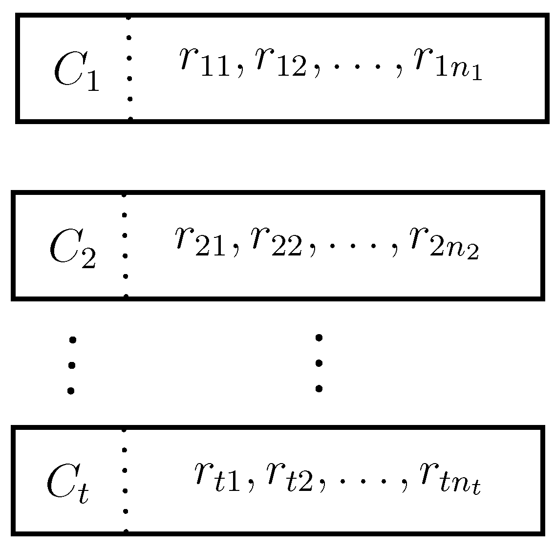
Among the attributes, we nominate the prioritization relationships. Then the collection of attributes is partitioned into t distinct categories $C_1,C_2,\dots ,C_t$ such that $C_i=\{r_{i1},r_{i2},\dots ,r_{i{n}_i}\}$, where $r_{ij}(j=1,2,\dots ,n_i)$ are the attributes in the category $C_i$.

Step 4.

On the basis of Equation (3), we compute the values of $l_i$ for each priority category $C_i$.

Step 5.

On the basis of Equation (4), we cumpute the weight $w_i$ of each category according to $l_i,i=1,2,\dots ,t$.

Step 6.

On the basis of Equation (1), we determine the importance of each attribute $r_i$.

Step 7.

By using the CPFWC operator (Equation (5)), we determine the overall importance of the alternatives and select the optimal alternative(s) in accordance with $s\left(I^{\left(r_i\right)}\right)(i=1,2,\dots m)$.

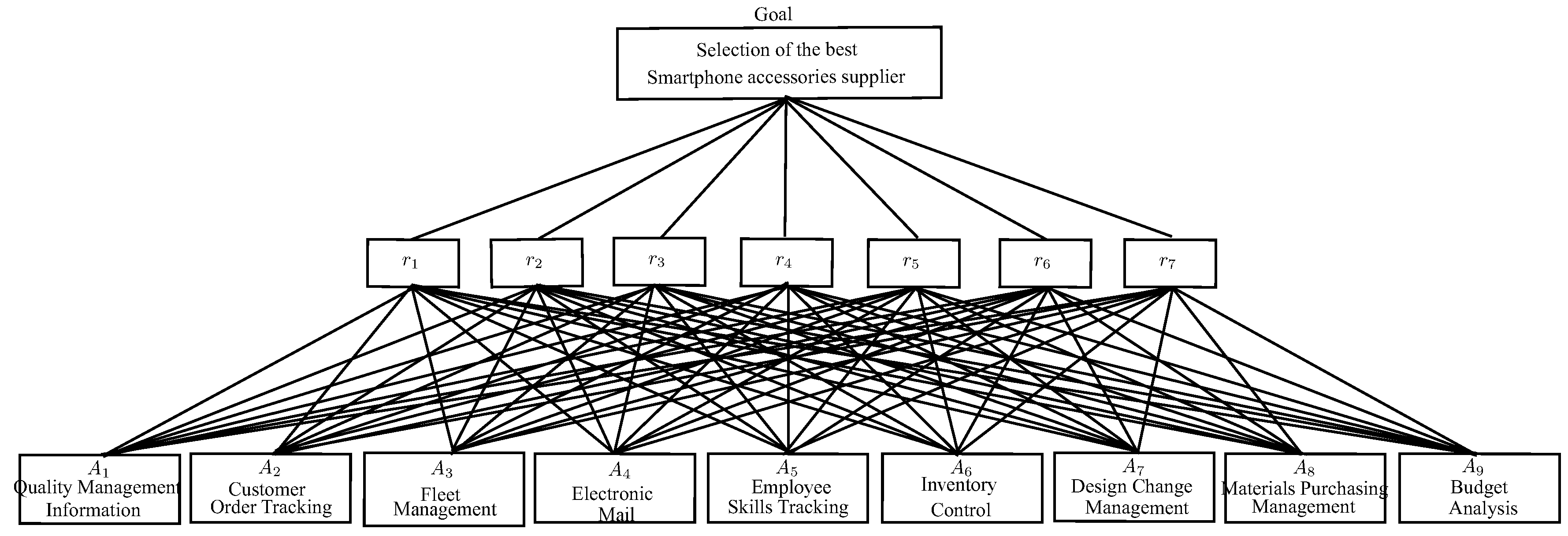
4.2. Illustrative Example

In this subsection, a numerical example is utilized to illustrate the validity of the developed MADM approach.

Midwest American Manufacturing Corp. (MAMC)’s information management steering committee wants to prioritize for development and implementation a set of nine information technology improvement projects (alternatives) $A_i(i=1,2,\dots ,9)$:

$A_1$

: Quality Management Information;

$A_2$

: Customer Order Tracking;

$A_3$

: Fleet Management;

$A_4$

: Electronic Mail;

$A_5$

: Employee Skills Tracking;

$A_6$

: Inventory Control;

$A_7$

: Design Change Management;

$A_8$

: Materials Purchasing Management;

$A_9$

: Budget Analysis.

which have been given by area managers. The committee is distressed that the projects (alternatives) are prioritized from maximum to minimum potential input to the firm’s strategic goal of achieving ambitious advantage in the industry. To determine the possible input of each project, a set of seven factors (attributes) $r_i(i=1,2,\dots ,7)$ are considered: Under the complex Pythagorean fuzzy circumstances, an expert is invited to evaluate these alternatives with complex Pythagorean fuzzy elements. Therefore, the complex Pythagorean fuzzy decision matrix is given in

Table 1. The evaluation information on the projects in a complex Pythagorean fuzzy environment.

	${\mathit{r}}_1$	${\mathit{r}}_2$	${\mathit{r}}_3$	${\mathit{r}}_4$
$A_1$	$(0.3e^{i2\pi \left(0.2\right)},0.4e^{i2\pi \left(0.6\right)})$	$(0.5e^{i2\pi \left(0.3\right)},0.4e^{i2\pi \left(0.8\right)})$	$\left(0.7e^{i2\pi \left(0.5\right)},0.2e^{i2\pi \left(0.4\right)}\right)$	$(0.9e^{i2\pi \left(0.4\right)},0.2e^{i2\pi \left(0.3\right)})$
$A_2$	$(0.6e^{i2\pi \left(0.3\right)},0.5e^{i2\pi \left(0.8\right)})$	$(0.8e^{i2\pi \left(0.4\right)},0.3e^{i2\pi \left(0.5\right)})$	$(0.7e^{i2\pi \left(0.3\right)},0.2e^{i2\pi \left(0.6\right)})$	$(0.5e^{i2\pi \left(0.2\right)},0.3e^{i2\pi \left(0.9\right)})$
$A_3$	$(0.6e^{i2\pi \left(0.4\right)},0.7e^{i2\pi \left(0.5\right)})$	$(0.7e^{i2\pi \left(0.2\right)},0.3e^{i2\pi \left(0.6\right)})$	$(0.6e^{i2\pi \left(0.3\right)},0.4e^{i2\pi \left(0.5\right)})$	$(0.7e^{i2\pi \left(0.5\right)},0.3e^{i2\pi \left(0.6\right)})$
$A_4$	$(0.5e^{i2\pi \left(0.4\right)},0.4e^{i2\pi \left(0.7\right)})$	$(0.8e^{i2\pi \left(0.5\right)},0.3e^{i2\pi \left(0.5\right)})$	$(0.6e^{i2\pi \left(0.6\right)},0.2e^{i2\pi \left(0.5\right)})$	$(0.9e^{i2\pi \left(0.2\right)},0.3e^{i2\pi \left(0.4\right)})$
$A_5$	$(0.7e^{i2\pi \left(0.1\right)},0.7e^{i2\pi \left(0.9\right)})$	$(0.5e^{i2\pi \left(0.3\right)},0.8e^{i2\pi \left(0.8\right)})$	$(0.7e^{i2\pi \left(0.6\right)},0.6e^{i2\pi \left(0.5\right)})$	$(0.7e^{i2\pi \left(0.4\right)},0.4e^{i2\pi \left(0.5\right)})$
$A_6$	$(0.5e^{i2\pi \left(0.6\right)},0.7e^{i2\pi \left(0.5\right)})$	$(0.2e^{i2\pi \left(0.9\right)},0.9e^{i2\pi \left(0.2\right)})$	$(0.6e^{i2\pi \left(0.5\right)},0.8e^{i2\pi \left(0.7\right)})$	$(0.8e^{i2\pi \left(0.7\right)},0.3e^{i2\pi \left(0.6\right)})$
$A_7$	$(0.8e^{i2\pi \left(0.8\right)},0.6e^{i2\pi \left(0.6\right)})$	$(0.7e^{i2\pi \left(0.4\right)},0.5e^{i2\pi \left(0.8\right)})$	$(0.6e^{i2\pi \left(0.4\right)},0.4e^{i2\pi \left(0.8\right)})$	$(0.5e^{i2\pi \left(0.4\right)},0.8e^{i2\pi \left(0.7\right)})$
$A_8$	$(0.4e^{i2\pi \left(0.3\right)},0.7e^{i2\pi \left(0.8\right)})$	$(0.1e^{i2\pi \left(0.7\right)},0.8e^{i2\pi \left(0.5\right)})$	$(0.8e^{i2\pi \left(0.3\right)},0.4e^{i2\pi \left(0.9\right)})$	$(0.6e^{i2\pi \left(0.7\right)},0.5e^{i2\pi \left(0.5\right)})$
$A_9$	$(0.9e^{i2\pi \left(0.2\right)},0.3e^{i2\pi \left(0.9\right)})$	$(0.8e^{i2\pi \left(0.3\right)},0.1e^{i2\pi \left(0.9\right)})$	$(0.2e^{i2\pi \left(0.7\right)},0.9e^{i2\pi \left(0.5\right)})$	$(0.5e^{i2\pi \left(0.4\right)},0.7e^{i2\pi \left(0.8\right)})$
	$r_5$	$r_6$	$r_7$
$A_1$	$(0.6e^{i2\pi \left(0.5\right)},0.3e^{i2\pi \left(0.8\right)})$	$(0.7e^{i2\pi \left(0.2\right)},0.3e^{i2\pi \left(0.4\right)})$	$(0.8e^{i2\pi \left(0.4\right)},0.1e^{i2\pi \left(0.3\right)})$
$A_2$	$(0.2e^{i2\pi \left(0.3\right)},0.9e^{i2\pi \left(0.8\right)})$	$(0.7e^{i2\pi \left(0.3\right)},0.4e^{i2\pi \left(0.8\right)})$	$(0.5e^{i2\pi \left(0.4\right)},0.6e^{i2\pi \left(0.7\right)})$
$A_3$	$(0.7e^{i2\pi \left(0.5\right)},0.5e^{i2\pi \left(0.6\right)})$	$(0.6e^{i2\pi \left(0.7\right)},0.2e^{i5\pi \left(0.5\right)})$	$(0.4e^{i2\pi \left(0.2\right)},0.9e^{i2\pi \left(0.9\right)})$
$A_4$	$(0.3e^{i2\pi \left(0.7\right)},0.8e^{i2\pi \left(0.6\right)})$	$(0.7e^{i2\pi \left(0.4\right)},0.1e^{i2\pi \left(0.9\right)})$	$(0.6e^{i2\pi \left(0.4\right)},0.7e^{i2\pi \left(0.5\right)})$
$A_5$	$(0.6e^{i2\pi \left(0.3\right)},0.6e^{i2\pi \left(0.4\right)})$	$(0.3e^{i2\pi \left(0.5\right)},0.9e^{i2\pi \left(0.8\right)})$	$(0.7e^{i2\pi \left(0.9\right)},0.4e^{i2\pi \left(0.4\right)})$
$A_6$	$(0.6e^{i2\pi \left(0.5\right)},0.3e^{i2\pi \left(0.8\right)})$	$(0.7e^{i2\pi \left(0.9\right)},0.4e^{i2\pi \left(0.4\right)})$	$(0.8e^{i2\pi \left(0.7\right)},0.1e^{i2\pi \left(0.4\right)})$
$A_7$	$(0.3e^{i2\pi \left(0.1\right)},0.8e^{i2\pi \left(0.8\right)})$	$(0.8e^{i2\pi \left(0.3\right)},0.4e^{i2\pi \left(0.8\right)})$	$(0.5e^{i2\pi \left(0.3\right)},0.6e^{i2\pi \left(0.8\right)})$
$A_8$	$(0.2e^{i2\pi \left(0.8\right)},0.5e^{i2\pi \left(0.6\right)})$	$(0.6e^{i2\pi \left(0.2\right)},0.5e^{i2\pi \left(0.7\right)})$	$(0.9e^{i2\pi \left(0.7\right)},0.3e^{i2\pi \left(0.6\right)})$
$A_9$	$(0.7e^{i2\pi \left(0.9\right)},0.5e^{i2\pi \left(0.4\right)})$	$(0.7e^{i2\pi \left(0.4\right)},0.6e^{i2\pi \left(0.5\right)})$	$(0.5e^{i2\pi \left(0.7\right)},0.8e^{i2\pi \left(0.5\right)})$

. The hierarchical structure of the given decision making problem is depicted in Figure 12.

Assume that a graph $G=(C,D)$, with seven factors (attributes) $C=\{r_1,r_2,r_3,r_4,r_5,r_6,r_7\}$ and a set of their relations (edges) $D=\{r_1{r}_2,r_1{r}_4,r_7{r}_6,r_7{r}_5,r_7{r}_4,r_7{r}_3,r_7{r}_2,r_7{r}_1\}$. Let $\mathcal{G}=(\mathcal{C},\mathcal{D})$ be a CPFG of a graph G, as in Figure 13.

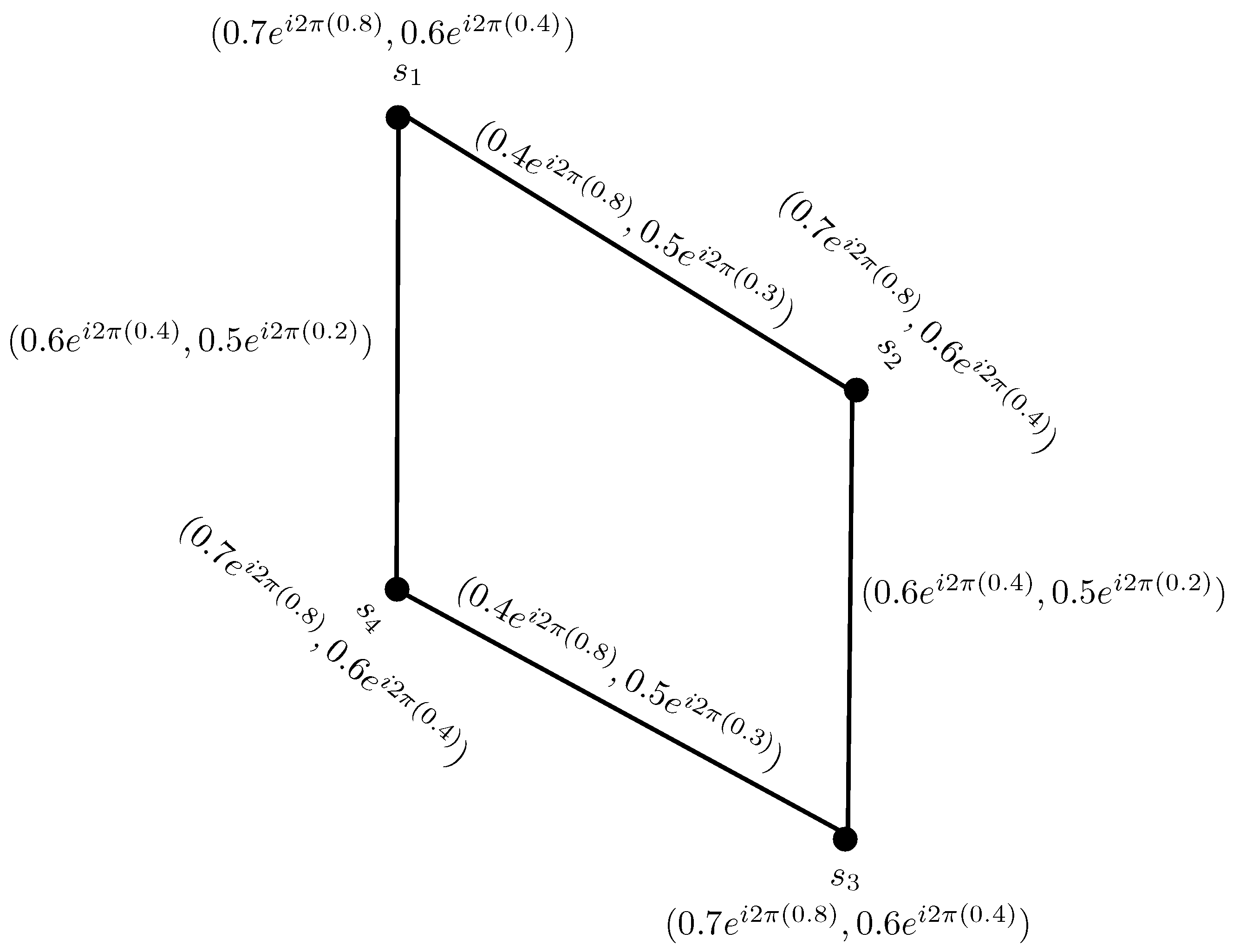
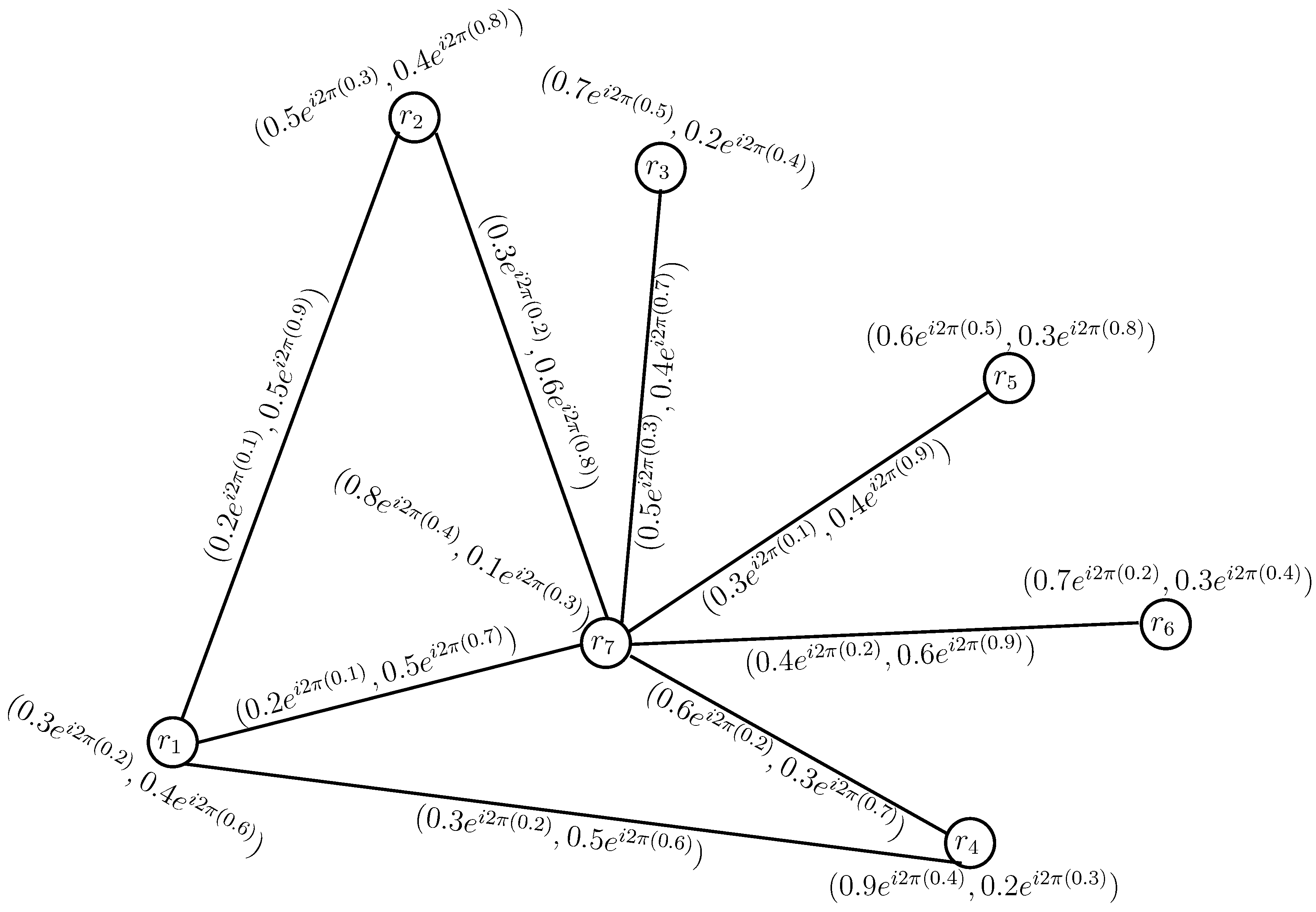
Step 1.

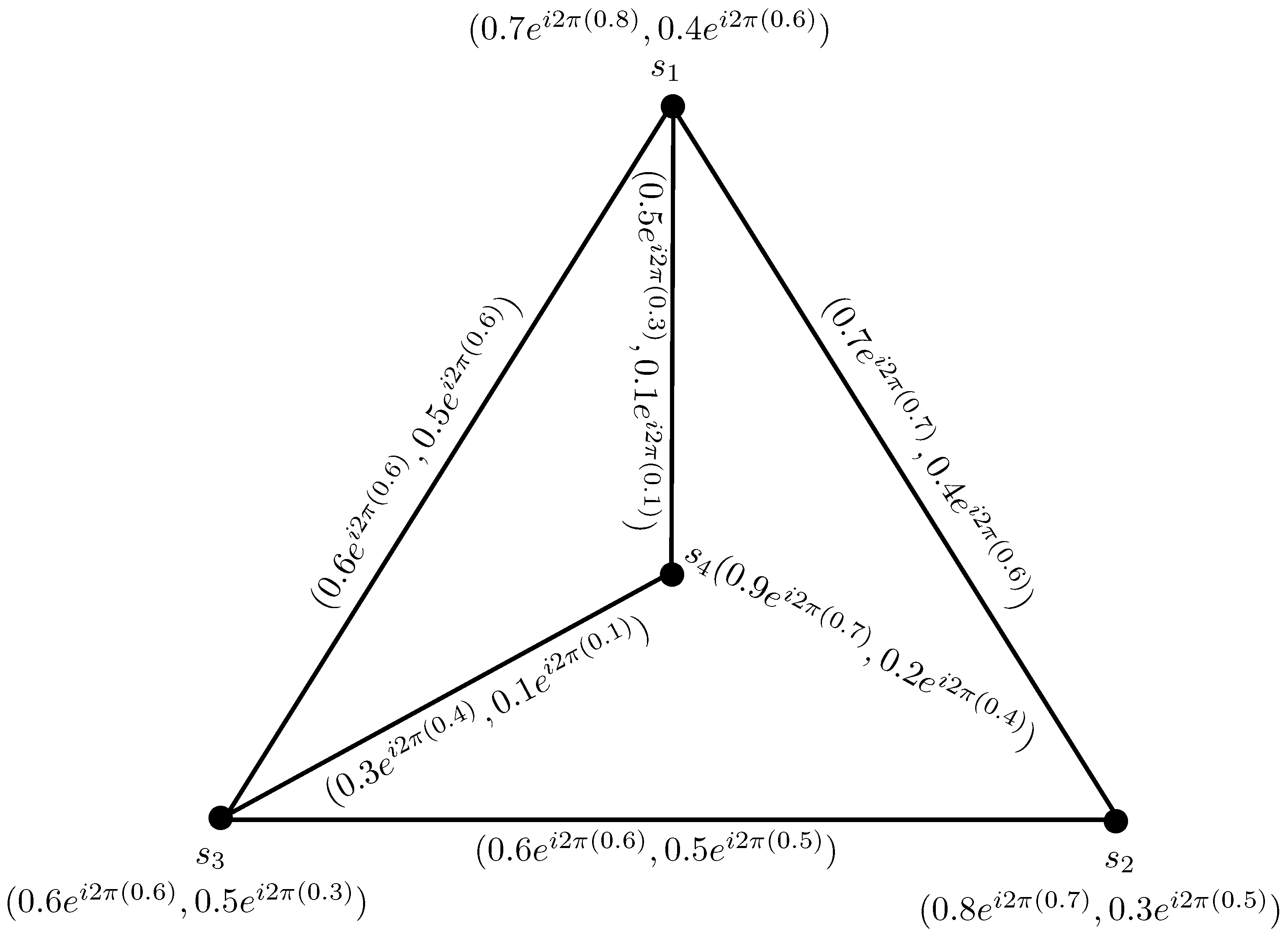
In graph of Figure 13, the degree of each attribute is determined as:

$$\begin{array}{c}\mathrm{d}\left(r_1\right)=(0.7e^{i2\pi \left(0.4\right)},1.5e^{i2\pi \left(2.2\right)}),\mathrm{d}\left(r_2\right)=(0.5e^{i2\pi \left(0.3\right)},1.1e^{i2\pi \left(1.7\right)}),\hfill \\ \mathrm{d}\left(r_3\right)=(0.5e^{i2\pi \left(0.3\right)},0.4e^{i2\pi \left(0.7\right)}),\mathrm{d}\left(r_4\right)=(0.9e^{i2\pi \left(0.4\right)},0.8e^{i2\pi \left(1.3\right)}),\hfill \\ \mathrm{d}\left(r_5\right)=(0.3e^{i2\pi \left(0.1\right)},0.4e^{i2\pi \left(0.9\right)}),\mathrm{d}\left(r_6\right)=(0.4e^{i2\pi \left(0.2\right)},0.6e^{i2\pi \left(0.9\right)}),\hfill \\ \mathrm{d}\left(r_7\right)=(2.3e^{i2\pi \left(1.1\right)},2.8e^{i2\pi \left(4.7\right)}).\hfill \end{array}$$

Utilizing Equation (2), normalize the above degrees as:

$$\begin{array}{c}\overline{\mathrm{d}}\left(r_1\right)=(0.1250e^{i2\pi \left(0.1429\right)},0.1974e^{i2\pi \left(0.1774\right)}),\overline{\mathrm{d}}\left(r_2\right)=(0.0893e^{i2\pi \left(0.1071\right)},0.1447e^{i2\pi \left(0.1371\right)}),\hfill \\ \overline{\mathrm{d}}\left(r_3\right)=(0.0893e^{i2\pi \left(0.1071\right)},0.0526e^{i2\pi \left(0.0565\right)}),\overline{\mathrm{d}}\left(r_4\right)=(0.1607e^{i2\pi \left(0.1429\right)},0.1053e^{i2\pi \left(0.1048\right)}),\hfill \\ \overline{\mathrm{d}}\left(r_5\right)=(0.0536e^{i2\pi \left(0.0357\right)},0.0526e^{i2\pi \left(0.0726\right)}),\overline{\mathrm{d}}\left(r_6\right)=(0.0714e^{i2\pi \left(0.0714\right)},0.0789e^{i2\pi \left(0.0726\right)}),\hfill \\ \overline{\mathrm{d}}\left(r_7\right)=(0.4107e^{i2\pi \left(0.3929\right)},0.3684e^{i2\pi \left(0.3790\right)}).\hfill \end{array}$$

Step 2.

Suppose that there exist prioritization complex Pythagorean fuzzy relations $C_1=\{r_1,r_4\},C_2=\left\{r_3\right\},C_3=\{r_2,r_7\},C_4=\{r_5,r_6\}$, $C_i>C_j$ if $i<j(i,j=1,2,3,4)$. So, $n_1=2,n_2=1,n_3=2,n_4=2$.

Step 3.

If $\phi$ is a minimum function, then utilizing Equation (3), we obtain

$$\begin{array}{c}{l}_0=\left(1e^{i2\pi \left(1\right)},0e^{i2\pi \left(0\right)}\right)\hfill \\ l_1=\left(0.1250e^{i2\pi \left(0.1429\right)},0.1974e^{i2\pi \left(0.1774\right)}\right)\hfill \\ l_2=\left(0.0893e^{i2\pi \left(0.1071\right)},0.0526e^{i2\pi \left(0.0565\right)}\right)\hfill \\ l_3=\left(0.0893e^{i2\pi \left(0.1071\right)},0.3684e^{i2\pi \left(0.3790\right)}\right)\hfill \\ l_4=\left(0.0536e^{i2\pi \left(0.0357\right)},0.0789e^{i2\pi \left(0.0726\right)}\right)\hfill \end{array}$$

Step 4.

On the basis of Equation (4), we calculate the weight of each category as:

$$\begin{array}{c}{w}_1=l_0=\left(1e^{i2\pi \left(1\right)},0e^{i2\pi \left(0\right)}\right)\hfill \\ w_2=l_0\otimes l_1=\left(0.1250e^{i2\pi \left(0.1429\right)},0.1974e^{i2\pi \left(0.1774\right)}\right)\hfill \\ w_3=l_0\otimes l_1\otimes l_2=\left(0.0112e^{i2\pi \left(0.0153\right)},0.2040e^{i2\pi \left(0.1859\right)}\right)\hfill \\ w_4=l_0\otimes l_1\otimes l_2\otimes l_3=\left(0.0010e^{i2\pi \left(0.0016\right)},0.4144e^{i2\pi \left(0.4162\right)}\right)\hfill \end{array}$$

Step 5.

If there is an alternative $A_1$, in which just attribute ‘$r_7$’ is most important, then $x_7=1$ and $x_i=0(i=1,2,\dots ,6)$. Also take $\xi \left(r_i{r}_j\right)=0.5$ for $i,j=1,2,\cdots ,7$ and $i\ne j$, then on the basis of Equation (1), the importance of all attributes are:

$$\begin{array}{ccc}\hfill I_1^{\left(A\right)}& =& ({\mu }_{\mathcal{C}}\left(r_1\right)e^{i{\alpha }_{\mathcal{C}}\left(r_1\right)},{\nu }_{\mathcal{C}}\left(r_1\right)e^{i{\beta }_{\mathcal{C}}\left(r_1\right)})x_1+{\overline{x}}_{{\mathcal{N}}_1}\hfill \\ & =& \left({\mu }_{\mathcal{D}}\left(r_1{r}_7\right)e^{i{\alpha }_{\mathcal{D}}\left(r_1{r}_7\right)},{\nu }_{\mathcal{D}}\left(r_1{r}_7\right)e^{i{\beta }_{\mathcal{D}}\left(r_1{r}_7\right)}\right)\xi \left(r_1{r}_7\right)x_7\hfill \\ & =& \left(0.1421e^{i2\pi \left(0.0708\right)},0.7071e^{i2\pi \left(0.8367\right)}\right),\hfill \end{array}$$

$$\begin{array}{ccc}\hfill I_2^{\left(A\right)}& =& ({\mu }_{\mathcal{C}}\left(r_2\right)e^{i{\alpha }_{\mathcal{C}}\left(r_2\right)},{\nu }_{\mathcal{C}}\left(r_2\right)e^{i{\beta }_{\mathcal{C}}\left(r_2\right)})x_2+{\overline{x}}_{{\mathcal{N}}_2}\hfill \\ & =& \left({\mu }_{\mathcal{D}}\left(r_2{r}_7\right)e^{i{\alpha }_{\mathcal{D}}\left(r_2{r}_7\right)},{\nu }_{\mathcal{D}}\left(r_2{r}_7\right)e^{i{\beta }_{\mathcal{D}}\left(r_2{r}_7\right)}\right)\xi \left(r_2{r}_7\right)x_7\hfill \\ & =& \left(0.2146e^{i2\pi \left(0.1421\right)},0.7746e^{i2\pi \left(0.8944\right)}\right),\hfill \end{array}$$

$$\begin{array}{ccc}\hfill I_3^{\left(A\right)}& =& ({\mu }_{\mathcal{C}}\left(r_3\right)e^{i{\alpha }_{\mathcal{C}}\left(r_3\right)},{\nu }_{\mathcal{C}}\left(r_3\right)e^{i{\beta }_{\mathcal{C}}\left(r_3\right)})x_3+{\overline{x}}_{{\mathcal{N}}_3}\hfill \\ & =& \left({\mu }_{\mathcal{D}}\left(r_3{r}_7\right)e^{i{\alpha }_{\mathcal{D}}\left(r_3{r}_7\right)},{\nu }_{\mathcal{D}}\left(r_3{r}_7\right)e^{i{\beta }_{\mathcal{D}}\left(r_3{r}_7\right)}\right)\xi \left(r_3{r}_7\right)x_7\hfill \\ & =& \left(0.3660e^{i2\pi \left(0.2146\right)},0.6325e^{i2\pi \left(0.8367\right)}\right),\hfill \end{array}$$

$$\begin{array}{ccc}\hfill I_4^{\left(A\right)}& =& ({\mu }_{\mathcal{C}}\left(r_4\right)e^{i{\alpha }_{\mathcal{C}}\left(r_4\right)},{\nu }_{\mathcal{C}}\left(r_4\right)e^{i{\beta }_{\mathcal{C}}\left(r_4\right)})x_4+{\overline{x}}_{{\mathcal{N}}_4}\hfill \\ & =& \left({\mu }_{\mathcal{D}}\left(r_4{r}_7\right)e^{i{\alpha }_{\mathcal{D}}\left(r_4{r}_7\right)},{\nu }_{\mathcal{D}}\left(r_4{r}_7\right)e^{i{\beta }_{\mathcal{D}}\left(r_4{r}_7\right)}\right)\xi \left(r_4{r}_7\right)x_7\hfill \\ & =& \left(0.4472e^{i2\pi \left(0.1421\right)}0.5477e^{i2\pi \left(0.8367\right)}\right),\hfill \end{array}$$

$$\begin{array}{ccc}\hfill I_5^{\left(A\right)}& =& ({\mu }_{\mathcal{C}}\left(r_5\right)e^{i{\alpha }_{\mathcal{C}}\left(r_5\right)},{\nu }_{\mathcal{C}}\left(r_5\right)e^{i{\beta }_{\mathcal{C}}\left(r_5\right)})x_5+{\overline{x}}_{{\mathcal{N}}_5}\hfill \\ & =& \left({\mu }_{\mathcal{D}}\left(r_5{r}_7\right)e^{i{\alpha }_{\mathcal{D}}\left(r_5{r}_7\right)},{\nu }_{\mathcal{D}}\left(r_5{r}_7\right)e^{i{\beta }_{\mathcal{D}}\left(r_5{r}_7\right)}\right)\xi \left(r_5{r}_7\right)x_7\hfill \\ & =& \left(0.2146e^{i2\pi \left(0.0708\right)},0.6325e^{i2\pi \left(0.9487\right)}\right),\hfill \end{array}$$

$$\begin{array}{ccc}\hfill I_6^{\left(A\right)}& =& ({\mu }_{\mathcal{C}}\left(r_6\right)e^{i{\alpha }_{\mathcal{C}}\left(r_6\right)},{\nu }_{\mathcal{C}}\left(r_6\right)e^{i{\beta }_{\mathcal{C}}\left(r_6\right)})x_6+{\overline{x}}_{{\mathcal{N}}_6}\hfill \\ & =& \left({\mu }_{\mathcal{D}}\left(r_6{r}_7\right)e^{i{\alpha }_{\mathcal{D}}\left(r_6{r}_7\right)},{\nu }_{\mathcal{D}}\left(r_6{r}_7\right)e^{i{\beta }_{\mathcal{D}}\left(r_6{r}_7\right)}\right)\xi \left(r_6{r}_7\right)x_7\hfill \\ & =& \left(0.2889e^{i2\pi \left(0.1421\right)}0.7746e^{i2\pi \left(0.9487\right)}\right),\hfill \end{array}$$

$$\begin{array}{ccc}\hfill I_7^{\left(A\right)}& =& ({\mu }_{\mathcal{C}}\left(r_7\right)e^{i{\alpha }_{\mathcal{C}}\left(r_7\right)},{\nu }_{\mathcal{C}}\left(r_7\right)e^{i{\beta }_{\mathcal{C}}\left(r_7\right)})x_7+{\overline{x}}_{{\mathcal{N}}_7}\hfill \\ & =& \left(0.8e^{i2\pi \left(0.4\right)},0.1e^{i2\pi \left(0.3\right)}\right).\hfill \end{array}$$

Step 6.

On the basis of Equation (5), we determine the overall importance of the alternative $A_1$ as:

$$\begin{array}{c}{I}^{\left(A_1\right)}={\vee }_{i=1}^7\left({\vee }_{j=1}^{n_i}(w_i\wedge I_{ij}^{\left(A\right)})\right)=\left(0.4472e^{i2\pi \left(0.1429\right)},0.2040e^{i2\pi \left(0.3000\right)}\right)\hfill \\ s\left(I^{\left(A_1\right)}\right)=0.1566.\hfill \end{array}$$

Furthermore, we determine the score functions of overall importance of the other alternatives $A_i(i=2,3,\dots ,9)$:

$$\begin{array}{c}s\left(I^{\left(A_2\right)}\right)=0.0397,s\left(I^{\left(A_3\right)}\right)=0.0412,s\left(I^{\left(A_4\right)}\right)=0.0433,s\left(I^{\left(A_5\right)}\right)=0.0341,s\left(I^{\left(A_6\right)}\right)=0.0307,\hfill \\ s\left(I^{\left(A_7\right)}\right)=0.0300,s\left(I^{\left(A_8\right)}\right)=0.0302,s\left(I^{\left(A_9\right)}\right)=0.0309.\hfill \end{array}$$

We rank the alternatives according to the score function of the overall importance of the alternatives $A_i(i=1,2,\dots ,9)$, as:

$$A_1\succ A_4\succ A_3\succ A_2\succ A_5\succ A_9\succ A_6\succ A_8\succ A_7$$

4.3. Comparative Analysis

Ashraf et al. [30] proposed the graph based decision making model, to accommodate single-valued neutrosophic values. We have utilized this approach to the above illustrative example and compared the decision results with the proposed approach of this paper for CPFGs. The results corresponding to these approaches are summarized in

Table 2. Comparative analysis.

Methods	Score of Alternatives	Ranking of Alternatives
Ashraf et al. [30]	0.7415  0.5810  0.5894  0.6115  0.5212  0.4390  0.2690  0.2781  0.4799	$A_1\succ A_4\succ A_3\succ A_2\succ A_5\succ A_9\succ A_6\succ A_8\succ A_7$
Our developed method	0.1566  0.0397  0.0412  0.0433  0.0341  0.0307  0.0300  0.0302  0.0309	$A_1\succ A_4\succ A_3\succ A_2\succ A_9\succ A_5\succ A_6\succ A_7\succ A_8$

.

From this comparative study, the results obtained by the existing approach coincide with the proposed one which validates the proposed approach. Hence, the proposed approach can be suitably utilized to solve the MCDM problems. The novelty of this decision making approach is that we have developed an MADM model with the interrelated attributes and described numerous relationships among the attributes by utilizing the corresponding graphical structures with complex Pythagorean fuzzy information.

5. Conclusions

CPFS as a generalized formation represents some general complex scenario. Our research paper enriches the area of fuzzy graph theory in several directions. Firstly, under the Pythagorean fuzzy circumstances, a novel concept of CPFGs has been proposed by combining PFGs and CFGs. CPFG, an extended structure of a fuzzy graph is more practical and flexible as compared to the classical, fuzzy, complex fuzzy and Pythagorean fuzzy models as it deals the vagueness with the membership and non-membership degrees whose ranges are generalized from real to the complex subset with a unit disc. Secondly, the novel concepts of regular and edge regular graphs have been defined with appropriate illustration and some of their crucial properties are examined within complex Pythagorean fuzzy contexts. Thirdly, some aggregation techniques have been investigated for CPFNs and, further, the complex Pythagorean fuzzy graphic structure has been utilized to depict the interrelated attributes in MADM and developed the multi-attribute decision making approach based on CPFG. Meanwhile, we interpret the relationships among the attributes and then derive a solution utilizing the MADM model based on the CPFGs. Taking into account the interval-valued vagueness, we shall extend the proposed research work to the complex interval-valued Pythagorean fuzzy setting and provide its applications further.

References

- Yager, R.R. Pythagorean fuzzy subsets. In Proceedings of the Joint IFSA World Congress and NAFIPS Annual Meeting, Edmonton, AB, Canada, 24–28 June 2013; pp. 57–61. [Google Scholar]
- Yager, R.R.; Abbasov, A.M. Pythagorean membership grades, complex numbers, and decision making. Int. J. Intell. Syst. 2013, 28, 436–452. [Google Scholar] [CrossRef]
- Yager, R.R. Pythagorean membership grades in multi-criteria decision making. IEEE Trans. Fuzzy Syst. 2014, 22, 958–965. [Google Scholar] [CrossRef]
- Atanassov, K.T. Intuitionistic fuzzy sets. Fuzzy Sets Syst. 1986, 20, 87–96. [Google Scholar] [CrossRef]
- Ramot, D.; Milo, R.; Fiedman, M.; Kandel, A. Complex fuzzy sets. IEEE Trans. Fuzzy Syst. 2002, 10, 171–186. [Google Scholar] [CrossRef]
- Yazdanbakhsh, O.; Dick, S. A systematic review of complex fuzzy sets and logic. Fuzzy Sets Syst. 2018, 338, 1–22. [Google Scholar] [CrossRef]
- Greenfield, S.; Chiclana, F.; Dick, S. Interval-valued complex fuzzy logic. In Proceedings of the IEEE International Conference on Fuzzy Systems, Vancouver, BC, Canada, 24–29 July 2016; pp. 1–6. [Google Scholar]
- Ramot, D.; Friedman, M.; Langholz, G.; Kandel, A. Complex fuzzy logic. IEEE Trans. Fuzzy Syst. 2003, 11, 450–461. [Google Scholar] [CrossRef]
- Alkouri, A.; Salleh, A. Complex intuitionistic fuzzy sets. AIP Conf. Proc. 2012, 14, 464–470. [Google Scholar]
- Alkouri, A.U.M.; Salleh, A.R. Complex Atanassov’s intuitionistic fuzzy relation. Abstr. Appl. Anal. 2013, 1–18. [Google Scholar] [CrossRef]
- Rani, D.; Garg, H. Distance measures between the complex intuitionistic fuzzy sets and its applications to the decision-making process. Int. J. Uncertain. Quantif. 2017, 7, 423–439. [Google Scholar] [CrossRef]
- Rani, D.; Garg, H. Complex intuitionistic fuzzy power aggregation operators and their applications in multi-criteria decision making. Expert Syst. 2018, 35, e12325. [Google Scholar] [CrossRef]
- Garg, H.; Rani, D. Some generalized complex intuitionistic fuzzy aggregation operators and their application to multi criteria decision-making process. Arab. J. Sci. Eng. 2019, 44, 2679–2698. [Google Scholar] [CrossRef]
- Kumar, T.; Bajaj, R.K. On complex intuitionistic fuzzy soft sets with distance measures and entropies. J. Math. 2014. [Google Scholar] [CrossRef]
- Ullah, K.; Mahmood, T.; Ali, Z.; Jan, N. On some distance measures of complex Pythagorean fuzzy sets and their applications in pattern recognition. Complex Intell. Syst. 2019. [Google Scholar] [CrossRef]
- Rosenfeld, A. Fuzzy Graphs, Fuzzy Sets and Their Applications; Zadeh, L.A., Fu, K.S., Shimura, M., Eds.; Academic Press: New York, NY, USA, 1975; pp. 77–95. [Google Scholar]
- Mordeson, J.N.; Peng, C.S. Operations on fuzzy graphs. Inf. Sci. 1994, 79, 159–170. [Google Scholar] [CrossRef]
- Yu, X.; Xu, Z. Graph-based multi-agent decision making. Int. J. Approx. Reason. 2012, 53, 502–512. [Google Scholar] [CrossRef]
- Habib, A.; Akram, M.; Farooq, A. q-Rung orthopair fuzzy competition graphs with application in the soil ecosystem. Mathematics 2019, 7, 91. [Google Scholar] [CrossRef]
- Naz, S.; Akram, M.; Smarandache, F. Certain notions of energy in single-valued neutrosophic graphs. Axioms 2018, 7, 50. [Google Scholar] [CrossRef]
- Naz, S.; Ashraf, S.; Akram, M. A novel approach to decision-making with Pythagorean fuzzy information. Mathematics 2018, 6, 95. [Google Scholar] [CrossRef]
- Akram, M.; Dar, J.M.; Naz, S. Pythagorean Dombi fuzzy graphs. Complex Intell. Syst. 2019. [Google Scholar] [CrossRef]
- Akram, M.; Dar, J.M.; Naz, S. Certain graphs under Pythagorean fuzzy environment. Complex Intell. Syst. 2019, 5, 127–144. [Google Scholar] [CrossRef]
- Akram, M.; Habib, A.; Ilyas, F.; Dar, J.M. Specific types of Pythagorean fuzzy graphs and application to decision-making. Math. Comput. Appl. 2018, 23, 42. [Google Scholar] [CrossRef]
- Akram, M.; Naz, S.; Davvaz, B. Simplified interval-valued Pythagorean fuzzy graphs with application. Complex Intell. Syst. 2019, 5, 229–253. [Google Scholar] [CrossRef]
- Thirunavukarasu, P.; Suresh, R.; Viswanathan, K.K. Energy of a complex fuzzy graph. Int. J. Math. Sci. Eng. Appl. 2016, 10, 243–248. [Google Scholar]
- Yaqoob, N.; Gulistan, M.; Kadry, S.; Wahab, H. Complex intuitionistic fuzzy graphs with application in cellular network provider companies. Mathematics 2019, 7, 35. [Google Scholar] [CrossRef]
- Yaqoob, N.; Akram, M. Complex neutrosophic graphs. Bull. Comput. Appl. Math. 2018, 6, 85–109. [Google Scholar]
- Yager, R.R. Prioritized aggregation operators. Int. J. Approx. Reason. 2008, 48, 263–274. [Google Scholar] [CrossRef]
- Samina, A.; Naz, S.; Rashmanlou, H.; Malik, M.A. Regularity of graphs in single valued neutrosophic environment. J. Intell. Fuzzy Syst. 2017, 33, 529–542. [Google Scholar]