Article

An Error Indicator-Based Adaptive Reduced Order Model for Nonlinear Structural Mechanics—Application to High-Pressure Turbine Blades

Safran Tech, Modelling and Simulation, Rue des Jeunes Bois, Châteaufort, 78114 Magny-Les-Hameaux, France
*
Author to whom correspondence should be addressed.
Math. Comput. Appl. 2019, 24(2), 41; https://doi.org/10.3390/mca24020041
Submission received: 26 February 2019 / Revised: 30 March 2019 / Accepted: 15 April 2019 / Published: 19 April 2019

Abstract

:
The industrial application motivating this work is the fatigue computation of aircraft engines’ high-pressure turbine blades. The material model involves nonlinear elastoviscoplastic behavior laws, for which the parameters depend on the temperature. For this application, the temperature loading is not accurately known and can reach values relatively close to the creep temperature: important nonlinear effects occur and the solution strongly depends on the used thermal loading. We consider a nonlinear reduced order model able to compute, in the exploitation phase, the behavior of the blade for a new temperature field loading. The sensitivity of the solution to the temperature makes the classical unenriched proper orthogonal decomposition method fail. In this work, we propose a new error indicator, quantifying the error made by the reduced order model in computational complexity independent of the size of the high-fidelity reference model. In our framework, when the error indicator becomes larger than a given tolerance, the reduced order model is updated using one time step solution of the high-fidelity reference model. The approach is illustrated on a series of academic test cases and applied on a setting of industrial complexity involving five million degrees of freedom, where the whole procedure is computed in parallel with distributed memory.

1. Introduction

The application of interest for this work is the lifetime computation of aircraft engines’ high-pressure turbine blades. Being located immediately downstream the combustion chamber, such parts undergo extreme thermal loading, with incoming fluid temperature higher than the material’s melting temperature. These blades are responsible for a large part of the maintenance budget of the engine, with temperature creep rupture and high-cycle fatigue [1,2] as possible failure causes. Various technological efforts have been spent to increase the durability of these blades as much as possible, such as thermal barrier coatings [3], advanced superalloys [4] and complex internal cooling channels [5,6], see Figure 1 for a representation of a high-pressure turbine blade.
Computing lifetime predictions for high-pressure turbine blades is a challenging task: meshes involve large numbers of degrees of freedom to account for local structures such as the internal cooling channels, the behavior laws are strongly nonlinear with many internal variables, and a large number of cycles has to be computed. Besides, the temperature loading is poorly known in the outlet section of the combustion chamber. Our team has proposed in [7] a nonintrusive reduced order model (ROM) strategy in parallel computation with distributed memory to mitigate the runtime issues: a domain decomposition method is used to compute the first cycle, and the reduced order model is used to speed up the computation of the following cycles, which can be considered as a reduced order model-based temporal extrapolation. As pointed out in [7], errors are accumulated during this temporal extrapolation. Moreover, quantifying the uncertainty on the lifetime with respect to some statistical description of the temperature loading using an already constructed reduced order model would introduce additional errors. In this context, error indicator-based enrichment of reduced order models is the topic of the present work.
Error estimation for reduced model predictions is a topic that receives interest in the scientific literature. The reduced basis method [9,10] for parametrized problems is a reduced order modeling method that intrinsically relies on efficient a posteriori error bounds of the error between the reduced prediction and the reference high-fidelity (HF) solution. This method consists of a greedy enrichment of a current reduced order basis by the high-fidelity solution at the parametric value that maximizes the error bound on a rich sampling of the parametric space. Being intensively evaluated, the error bound must be computed in computational complexity independent of the number of degrees of freedom of the high-fidelity reference. Initially proposed for elliptic coercive partial differential equations [11], where the error bound is the dual norm of the residual divided by a lower bound of the stability constant, the method has been adapted to problems of increased difficulty, with the derivation of certified error bounds for the Boussinesq equation [12], the Burger’s equation [13], and the Navier–Stokes equations [14]. Numerical stability of such error estimations with respect to round-off error can be an issue in nonlinear problems, which was investigated in [15,16,17,18].
Even if it is not a requirement for their execution, error estimation is a desired feature for all the other reduced order modeling methods. In proper generalized decomposition (PGD) methods [19], error estimation based on the constitutive relation error method is available [20,21,22]. In proper orthogonal decomposition (POD)-based reduced order modeling methods [23,24], error estimators have been developed for linear-quadratic optimal control problems [25], the approximation of mixte finite element problems [26], the optimal control of nonlinear parabolic partial differential equations [27], and for the reduction of magnetostatic problems [28] and Navier–Stokes equations [29]. To reduce nonlinear problems, the POD has been coupled with reduced integration strategies called hyperreduction, for which error estimates in constitutive relation have been proposed [30,31]. A priori sensitivity studies for POD approximations of quasi-nonlinear parabolic equations are also available [32].
The contribution of this work consists in the construction of a new error indicator, adapted to the model order reduction of nonlinear structural mechanics, where we are interested in the prediction of the dual quantities such as the cumulated plasticity or the stress tensor. These dual quantities need a reconstruction step to be represented on the complete structure of interest, usually done using a Gappy-POD algorithm based on the reduced solution. We illustrate that the ROM-Gappy-POD residual of the quantities of interest is highly correlated to the error in our cases. From this observation, we propose a calibration step, based on the data computed during the offline stage of the reduced order modeling, to construct an error indicator adapted to the considered problem and configuration. This error indicator is then used in enrichment strategies that improve the accuracy of the reduced order model prediction, when nonparametrized variations of the temperature field are considered in the online stage.
The problem of interest, the evolution of an elastoviscoplastic body under a time-dependent loading, in presented in Section 2. Then, the a posteriori reduced order modeling of this problem is detailed in Section 3. Section 4 presents the proposed error indicator, and the enrichment strategy based upon it. The performances of this error indicator and its ability to improve the quality of the reduced order model prediction via enrichment are illustrated in two numerical experiments involving elastoviscoplastic materials in Section 5. Finally, conclusions and prospects are given in Section 6.

2. High-Fidelity Elastoviscoplastic Model

We consider the model introduced in [7], which we briefly recall below for the sake of completeness. The structure of interest is noted Ω and its boundary Ω , where Ω = Ω D Ω N such that Ω D Ω N = , see Figure 2.
Prescribed zero displacements are imposed on Ω D , prescribed tractions T N are imposed on Ω N and volumic forces are imposed to the structure Ω , in the form of a time-dependent loading. Assuming small deformations, the evolution of the structure Ω is governed by equations
ϵ ( u ) = 1 2 u + T u in Ω × [ 0 , T ] ( compatibility ) ,
div σ + f = 0 in Ω × [ 0 , T ] ( equilibrium ) ,
σ = σ ( ϵ ( u ) , y ) in Ω × [ 0 , T ] ( behavior law ) ,
u = 0 in Ω D × [ 0 , T ] ( prescribed zero displacement ) ,
σ · n = T N in Ω N × [ 0 , T ] ( prescribed traction ) ,
u = 0 , y = 0 in Ω at t = 0 ( initial condition ) ,
where σ is the Cauchy stress tensor, ϵ is the linear strain tensor, n is the exterior normal on Ω , y denotes the internal variables of the behavior law, and u is the displacement solution.
Consider H 0 1 ( Ω ) = { v L 2 ( Ω ) | v x i L 2 ( Ω ) , 1 i 3 and v | Ω D = 0 } . We introduce a finite element basis { φ i } 1 i N , such that V : = Span φ i 1 i N is a conforming approximation of H 0 1 ( Ω ) 3 . In what follows, bold symbols are used to refer to vectors. Using the Galerkin method, problem (1a)–(1f) leads to a system of nonlinear equations, numerically solved using the following Newton algorithm:
D F D u u k u k + 1 - u k = - F u k ,
where u k V is the k-th iteration of the discretized displacement field at the considered time-step and u k = u i k 1 i N R N is such that u k = i = 1 N u i k φ i ,
D F D u u k i j = Ω ϵ φ j : K ϵ ( u k ) , y : ϵ φ i , 1 i , j N ,
where K ϵ ( u k ) , y is the local tangent operator, and
F i u k = Ω σ ϵ ( u k ) , y : ϵ φ i - Ω f · φ i - Ω N T N · φ i , 1 i N .
The Newton algorithm stops when the norm of the residual divided by the norm of the external forces vector is smaller than a user-provided tolerance, denoted ϵ Newton HFM .
In Equation (2), f, T N , u k and y from Equation (4) are known quantities and contain the time-dependency of the solution. Notice that the computation of the functions u k , y σ ϵ ( u k ) , y and u k , y K ϵ ( u k ) , y requires solving ordinary differential equations, whose complexity depends on the behavior law modeling the considered material.
In our application, the quantities of interest are not the displacement fields u, but rather the dual quantities stress tensor field σ and cumulated plasticity field, denoted p. The finite element software used to generate the high-fidelity solutions u is Zebulon, which contains a domain decomposition solver able to solve large scale problems, and the behavior laws are computed using Z-mat; both solvers belong to the Z-set suite [33].

3. Reduced Order Modeling

Reduced order modeling techniques are usually decomposed in two stages: the offline stage, where information from the high-fidelity model (HFM) is learned, and the online stage, where the reduced order model is constructed and exploited. In the offline stage, computationally demanding tasks occur, whereas the online stage is required to be efficient, in the sense that only operations in computational complexity independent of the number N of degrees of freedom of the high-fidelity model are allowed.
In what follows, we consider a posteriori reduced order modeling, which means that our reduced model involves an efficient Galerkin method no longer written in the finite element basis ( φ i ) 1 i N , but on a reduced order basis ( ψ i ) 1 i n , with n N , adapted to the problem at hand. To generate this basis, the high-fidelity problem (1a)–(1f) is solved for given configurations. In the general case, the variations between the candidate configurations are quantified using a low-dimensional parametrization, leading to a parametrized reduced order model. In this work, we consider nonparametrized variations between the configurations of interest, which we call variability and denote μ . The variability contains the time step, as well as a nonparametrized description of the configuration, which in our case is the loading referred as a label. For instance, μ = { t = 3 , computation 1 } , means that we consider the third time step of the configuration “computation 1”, for which we have a description of the loading (center, axis and speed of rotation, temperature, and pressure fields in our applications). We denote by P off . the set of variabilities encountered during the offline stage.
The reduced Newton algorithm reads
D F μ D u u ^ μ k u ^ μ k + 1 - u ^ μ k = - F μ u ^ μ k ,
where u ^ μ k V ^ : = Span ψ i 1 i n is the k-th iteration of the reduced displacement field for the considered time-step and u ^ μ k = u ^ μ , i k 1 i n R n is such u ^ μ k = i = 1 n u ^ μ , i k ψ i ,
D F μ D u u ^ μ k i j = Ω ϵ ψ j : K ϵ ( u ^ μ k ) , y μ : ϵ ψ i , 1 i , j n ,
and
F μ , i u ^ k = Ω σ ϵ ( u ^ μ k ) , y μ : ϵ ψ i - Ω f μ · ψ i - Ω N T N , μ · ψ i , 1 i n .
The reduced Newton algorithm stops when the norm of the reduced residual divided by the norm of the reduced external forces vector is smaller than a user-provided tolerance, denoted ϵ Newton ROM . In Equations (5)–(7), the online variability μ consists in the considered time step, the pressure field T N , μ , the centrifugal effects f μ , and the temperature field in the internal variables y μ .
Ensuring the efficiency of Equation (5) can be a complicated task, in particular for nonlinear problems, that requires methodologies recently proposed in the literature. For instance, the integrals in Equations (6) and (7) are computed in computational complexity dependent on N in the general case. We briefly present the choices made in our previous work [7]: the offline stage is composed of the following steps
  • Data generation: this corresponds to the generation of the numerical approximation of the solutions to Equation (1a)–(1f), using the Newton algorithm (2). Multiple temporal solutions can be considered, for different loading conditions. The set of theses solutions { u μ i } 1 i N c is called the snapshots set.
  • Data compression: this corresponds to the generation of the reduced order basis, usually obtained by looking for a hidden low-rank structure of the snapshots set. In this work, we consider the snapshot POD, see Algorithm 1 and [23,24].
  • Operator compression: this step enables the efficient construction of (5), usually by replacing the computationally demanding integral evaluations by adapted approximation evaluated in computational complexity independent of N. In this work, we consider the empirical cubature method (ECM, see [34]), a method close to the energy conserving sampling and weighting (ECSW, see [35,36,37]) proposed earlier. Consider the vector of reduced internal forces appearing in (7):
    F ^ μ , i int : = Ω σ ϵ ( u ^ μ ) , y μ ( x ) : ϵ ψ i ( x ) d x e E k = 1 n e ω k σ ϵ ( u ^ μ ) , y μ ( x k ) : ϵ ψ i ( x k ) , 1 i n ,
    where the right-hand side is the high-fidelity quadrature formula used for numerical evaluation. In (8), the stress tensor σ ϵ ( u ^ μ ) , y μ for the considered reduced solution u ^ μ at variability μ and internal variables y μ is seen as a function of space, and E denotes the set of elements of the mesh, n e denotes the number of integration points for the element e, ω k and x k are the integration weights and points of the considered element. The ECM consists of replacing this high-fidelity quadrature (8) by an approximation adapted to the snapshots { u μ i } 1 i N c and the reduced order basis { ψ i } 1 i n , and involving a small number of integration points:
    F ^ μ , i int ( t ) k = 1 d ω ^ k σ ϵ ( u ^ μ ) , y μ ( x ^ k ) : ϵ ψ i ( x ^ k ) , 1 i n ,
    where d e E n e , the reduced integration points x ^ k , 1 k d , are taken among the integration points of the high-fidelity quadrature (8) and the reduced integration weights ω ^ k are positive. We now briefly present how this reduced quadrature formula is obtained and we refer to [7,34] for more details. We denote h q : = σ ϵ ( u μ ( q / / n ) + 1 ) , y : ϵ ψ ( q % n ) + 1 L 2 ( Ω ) , where / / and % are respectively the quotient and the remainder of the Euclidean division, Z is a subset of [ 1 ; N G ] of size d, with N G the number of integration points, and J Z R n N c × d and g N n N c are such that for all 1 q n N c and all 1 k d ,
    J Z = h q ( x Z k ) 1 q n N c , 1 k d , g = Ω h q 1 q n N c ,
    where Z k denotes the k -th element of Z and where we recall that n is the number of snapshot POD modes. Let ω ^ R + d . From the introduced notation, J Z ω ^ q = k = 1 d ω ^ k σ ϵ ( u μ ( q / / n ) + 1 ) , y ( x Z k ) : ϵ ψ ( q % n ) + 1 ( x Z k ) , 1 q n N c , which is a candidate approximation for Ω σ ϵ ( u μ ( q / / n ) + 1 ) , y : ϵ ψ ( q % n ) + 1 = g q , 1 q n N c . The best reduced quadrature formula of length d for the reduced internal forces vector is obtained as (c.f. [34], Equation (23))
    ω ^ , Z = arg min ω ^ > 0 , Z [ 1 ; N G ] J Z ω ^ - g 2 ,
    where · 2 stands for the Euclidean norm. Taking the length of the reduced quadrature formula in the objective function yields a NP-hard optimization problem, see ([35], Section 5.3), citing [38]. To produce a reduced quadrature formula in a controlled return time, we consider a nonnegative orthogonal matching pursuit algorithm, see ([39], Algorithm 1) and Algorithm 2 below, a variant of the matching pursuit algorithm [40] tailored to the nonnegative requirement.
    A reduced quadrature is also used to accelerate the integral computation in (6). The remaining integral computations in (5) are Ω f μ · ψ i and Ω N T N , μ · ψ i . They do not depend on the current solution, but only on the loading of the online variability μ , which is no longer efficient for nonparametrized variabilities. However, in our context of large scale nonlinear mechanics, these integrals are computed very fast with respect to the ones requiring behavior law resolutions, see Remark 1.
Algorithm 1: Data compression by snapshot proper orthogonal decomposition (POD).
   Input: tolerance ϵ POD , snapshots set { u μ i } 1 i N c
   Output: reduced order basis { ψ i } 1 i n
1.
Compute the correlation matrix C i , j = Ω u μ i · u μ j , 1 i , j N c
2.
Compute the n largest eigenvalues λ i , 1 i n , and associated orthonormal eigenvectors ξ i , 1 i n , of C such that n = max n 1 , n 2 , where n 1 and n 2 are respectively the smallest integers such that i = 1 n 1 λ i 1 - ϵ POD 2 i = 1 N c λ i and λ n 2 ϵ POD 2 λ 0
3.
Compute the reduced order basis ψ i ( x ) = 1 λ i N c j = 1 N c u μ j ( x ) ξ i , j , 1 i n
Algorithm 2: Nonnegative orthogonal matching pursuit.
Mca 24 00041 i027
For the primal quantity displacement u, we can identify the solution of the reduced problem u ^ μ k R n with the reconstruction on the complete domain Ω : u ^ μ k = i = 1 n u ^ μ , i k ψ i . For the dual quantities, such identification does not exist. However, the behavior law has already been evaluated at the integration point of the reduced quadrature x ^ k , 1 k d . Since the evaluations are computed during the resolution of the reduced problem, we denote them by hats. For instance for the cumulated plasticity, p ^ μ R d is such that p ^ μ , k is computed by the online evaluation of the behavior law solver at the reduced integration points x ^ k , 1 k d . To recover the cumulated plasticity on the complete structure Ω , a ROM-Gappy-POD procedure is used to reconstruct the fields on the complete domain, see Algorithms 3 and 4 and [41] for the original presentation of the Gappy-POD. In step 2 of Algorithm 3, EIM denotes the empirical interpolation method [42,43] and the set of integration point whose indices have been selected is still denoted { x ^ k } 1 k m p , where n p m p n p + d . The dual quantities predicted by the reduced order model and reconstructed on the complete structure are denoted with tildes, for instance p ˜ μ for the cumulated plasticity.
The ROM-Gappy-POD reconstruction is well-posed, since the linear system considered in the online stage of Algorithm 4 is invertible, see ([7], Proposition 1).
An interesting feature of our framework is the ability for it to be used sequentially or in parallel with distributed memory. Independently of the high-fidelity solver, the solutions can be partitioned between some subdomains and the reduced order framework can treat the data in parallel. The MPI communications are limited to the computation of the scalar products in line 1 of Algorithm 1 for the offline stage, and the scalar products in (6) and (7) in the online stage. Furthermore, these scalar products are well adapted to parallel processing: each process computes its independently contribution on its respective subdomain, and the interprocess communication is limited to an all-to-all transfer of a scalar. All the remaining operations in our framework are treated in parallel with no communication, in particular in the operator compression step, reduced quadrature formulae are constructed independently. A natural use for the parallel framework is in coherence with domain decomposition solvers (potentially from commercial codes), which conveniently produce solutions partitioned in subdomains. Actually in our framework, the three steps of the offline stage (data generation, data compression and operator compression), the online stage, the post-treatment and the visualization are all treated in parallel with distributed memory, see [7] for more details.
Algorithm 3: Dual quantity reconstruction of the cumulated plasticity p: offline stage of the reduced order model (ROM)-Gappy-POD.
   Input: tolerance ϵ Gappy - POD , cumulated plasticity snapshots set { p μ i } 1 i N c , indices of the integration points of the reduced quadrature formula
   Output: indices for online material law computation, ROM-Gappy-POD matrix
1
Apply the snapshot POD (Algorithm 1) on the high-fidelity snapshots { p μ i } 1 i N c to obtain the vectors ψ i p , 1 i n p , orthonormal with respect to the L 2 ( Ω ) -inner product
2
Apply the EIM to the collection of vectors ψ i p , 1 i n p , to select n p distinct indices and complete (without repeat) this set of indices by the indices of the integration points of the reduced quadrature formula
3
Construct the matrix M N n p × n p such that M i , j = k = 1 m p ψ i p ( x ^ k ) ψ j p ( x ^ k ) (Gappy scalar product of the POD modes)
Algorithm 4: Dual quantity reconstruction of the cumulated plasticity p: online stage of the ROM-Gappy-POD.
   Input: online variability μ , indices for online material law computation, ROM-Gappy-POD matrix
   Output: reconstructed value for p on the complete domain Ω
1
Construct b μ R n p , where b μ , i = k = 1 m p ψ i p ( x ^ k ) p ^ μ , k , and  p ^ μ R m p is such that p ^ μ , k is the online prediction of p at variability μ and integration point x ^ k (from the online evaluation of the behavior law solver)
2
Solve the (small) linear system: M z μ = b μ
3
Compute the reconstructed value for p on the complete subdomain Ω as p ˜ μ : = i = 1 n p z μ , i ψ i p

4. A Heuristic Error Indicator

We look for an efficient error indicator in this context of general nonlinearities and nonparametrized variabilities. In model order reduction techniques, error estimation is an important feature, that becomes interesting under the condition that it can be computed in complexity independent of the number of degrees of freedom N of the high-fidelity model.

4.1. First Results on Errors and Residuals

We recall some notations introduced so far: bold symbols refer to vectors ( p μ is the vector of components the value of the HF cumulated plasiticity field at reduced integration points), hats refer to quantities computed by the reduced order model ( u ^ μ is the reduced displacement and p ^ μ is the vector of components the value of the reduced cumulated plasticity at the reduced quadrature points), whereas tildes refer to dual quantities reconstructed by Gappy-POD (for instance p ˜ ). Bold and tilde symbols, for instance p ˜ μ , refer to the vectors of components the reconstructed dual quantities on the reduced integration points: p ˜ μ , k = p ˜ μ ( x ^ k ) , 1 k m p . Notice that in the general case, p ˜ μ p ^ μ : this discrepancy is at the base of our proposed error indicator. A table of notations is provided at the end of the document.
A quantification for the prediction relative error is defined as
E μ p : = p μ - p ˜ μ L 2 ( Ω ) p μ L 2 ( Ω ) if  ∥ p μ L 2 ( Ω ) 0 p μ - p ˜ μ L 2 ( Ω ) max μ P off . p μ L 2 ( Ω ) otherwise , ,
where we recall that p μ and p ˜ μ are respectively the high-fidelity and reduced predictions for the cumulated plasticity field at the variability μ , and P off . is the set of variabilities encountered during the offline stage.
Define the ROM-Gappy-POD residual as
E μ p : = p ˜ μ - p ^ μ 2 p ^ μ 2 i f p ^ μ 2 0 p ˜ μ - p ^ μ 2 max μ P off . p ^ μ 2 otherwise , ,
where · 2 denotes the Euclidean norm. Notice that the relative error E μ p involves fields and L 2 -norms whereas the ROM-Gappy-POD residual E μ p involves vectors of dual quantities in the set of reduced integration points and Euclidean norms. In (13), p ˜ μ - p ^ μ 2 is the error between the online evaluation of the cumulated plasticity by the behavior law solver: p ^ μ , and the reconstructed prediction at the reduced integration points x ^ k : p ˜ μ , 1 k m p . Let B R m p × n p such that B k , i = ψ i p ( x ^ k ) , 1 k m p , 1 i n p ; by definition, p ˜ μ , k = i = 1 n p z μ , i ψ i p ( x ^ k ) = B z μ k , 1 k m p . From Algorithm 3, M = B T B and from Algorithm 4, b μ = B T p ^ μ , so that z μ = B T B - 1 B T p ^ μ , which is the solution of the following unconstrained least-square optimization: z μ : = arg z R n min B z - p ^ μ 2 2 . Hence, in (13), p ˜ μ - p ^ μ 2 is the norm of the residual of the considered least-square optimization.
Suppose K : = { p μ , for all possible variabilities μ } is a compact subset of L 2 ( Ω ) and define the Kolmogorov n-width by d n ( K ) L 2 ( Ω ) : = inf dim ( W ) = n d ( K , W ) L 2 ( Ω ) , where d ( K , W ) L 2 ( Ω ) : = sup v K inf w W v - w L 2 ( Ω ) , with W a finite-dimensional subspace of L 2 ( Ω ) . The Kolmogorov n-width is an object from approximation theory; a presentation and discussion in a reduced order modeling context can be found in [44]. Denote also Π μ : = p μ , ψ i p L 2 ( Ω ) 1 i n p R n p , where we recall that ψ i p 1 i n p are the Gappy-POD modes obtained by Algorithm 3 and where · , · L 2 ( Ω ) denotes the L 2 ( Ω ) inner-product. All the dual quantities being computed by the high-fidelity solver at the N G integration points, they have finite values at these points. Unlike the primal displacement field, the dual quantities are not directly expressed in a finite element basis, but through their values on the integration points. For pratical manipulations, we express the dual quantity fields as a constant on each polyhedron obtained as a Voronoi diagram in each element of the mesh, with seeds the integration points; the constants corresponding to the value of the dual quantity on the corresponding integration point.
We first control the numerator in the relative error E μ p with respect to the numerator in the ROM-Gappy-POD residual E μ p in Proposition 1.
Proposition 1.
There exist two positive constants C 1 and C 2 independent of μ (but dependent on n p ) such that
p μ - p ˜ μ L 2 ( Ω ) 2 C 1 B z μ - p ^ μ 2 2 + C 1 p μ - p ^ μ 2 2 + C 2 d ( K , Span { ψ i p } 1 i n p ) L 2 ( Ω ) 2 .
Proof. 
There holds
p μ - p ˜ μ L 2 ( Ω ) 2 2 i = 1 n p p μ , ψ i p L 2 ( Ω ) - z μ , i ψ i p L 2 ( Ω ) 2 + 2 p μ - i = 1 n p p μ , ψ i p L 2 ( Ω ) ψ i p L 2 ( Ω ) 2
= 2 i = 1 n p p μ , ψ i p L 2 ( Ω ) - z μ , i 2 + 2 inf w Span { ψ i p } 1 i n p p μ - w L 2 ( Ω ) 2
2 i = 1 n p Π μ , i - z μ , i 2 + 2 sup v K inf w Span { ψ i p } 1 i n p v - w L 2 ( Ω ) 2
= 2 M - 1 M Π μ - z μ 2 2 + 2 d ( K , Span { ψ i p } 1 i n p ) L 2 ( Ω ) 2
= 2 M - 1 B T B Π μ - p μ + p μ - p ^ μ + p ^ μ - B z μ 2 2 + 2 d ( K , Span { ψ i p } 1 i n p ) L 2 ( Ω ) 2
6 M - 1 B T 2 2 B Π μ - p μ 2 2 + p μ - p ^ μ 2 2 + B z μ - p ^ μ 2 2 + 2 d ( K , Span { ψ i p } 1 i n p ) L 2 ( Ω ) 2
C 1 B z μ - p ^ μ 2 2 + C 1 p μ - p ^ μ 2 2 + C 2 d ( K , Span { ψ i p } 1 i n p ) L 2 ( Ω ) 2 ,
where the triangular inequality and the Jensen inequality on the square function have been applied in (15a), and between (15e) and (15f). In (15g), the term B Π μ - p μ 2 2 has been incorporated in the term C 2 d ( K , Span { ψ i p } 1 i n p ) L 2 ( Ω ) 2 . This can be done since
B Π μ - p μ 2 2 = k = 1 m p p μ ( x ^ k ) - i = 1 n p p μ , ψ i p L 2 ( Ω ) ψ i p ( x ^ k ) 2 1 min 1 k m p ν k k = 1 N g ν k p μ ( x k ) - i = 1 n p p μ , ψ i p L 2 ( Ω ) ψ i p ( x k ) 2 = 1 min 1 k m p ν k Ω p μ ( x ) - i = 1 n p p μ , ψ i p L 2 ( Ω ) ψ i p ( x ) 2 d x 1 min 1 k m p ν k d ( K , Span { ψ i p } 1 i n p ) L 2 ( Ω ) 2 ,
where ν k denotes the volume of the cell of the Voronoi diagram associated with integration point x ^ k . ☐
We now control the numerator in the ROM-Gappy-POD residual E μ p with respect to the numerator in the relative error E μ p in Proposition 1, leading to Corollary 1, which provides a sense a consistency: without any error in the reduced prediction, the ROM-Gappy-POD residual E μ p is zero.
Proposition 2.
There exist two positive constants K 1 and K 2 independent of μ such that
p ˜ μ - p ^ μ 2 2 K 1 p μ - p ˜ μ L 2 ( Ω ) 2 + K 2 p μ - p ^ μ 2 2 .
Proof. 
There holds
p ˜ μ - p ^ μ 2 2 2 B z μ - p μ 2 2 + 2 p μ - p ^ μ 2 2 2 min 1 k m p ν k k = 1 m p ν k p μ ( x ^ k ) - i = 1 n p z μ , i ψ i p ( x ^ k ) 2 + 2 p μ - p ^ μ 2 2 2 min 1 k m p ν k Ω p μ ( x ) - i = 1 n p z μ , i ψ i p ( x ) 2 d x + 2 p μ - p ^ μ 2 2 = K 1 p μ - p ˜ μ L 2 ( Ω ) 2 + K 2 p μ - p ^ μ 2 2 .
 ☐
Corollary 1.
Suppose that the reduced solution is exact up to the considered time step at the online variability μ: p μ = p ˜ μ in L 2 ( Ω ) . In particular, the behavior law solver has been evaluated with the exact strain tensor and state variables at the integration points x k , leading to p ^ μ ( x ^ k ) = p μ ( x ^ k ) , 1 k m d . From Proposition 2, p ˜ μ - p ^ μ 2 = 0 , and E μ p = 0 .

4.2. A Calibrated Error Indicator

As we will illustrate in Section 5, the evaluations of the ROM-Gappy-POD residual E μ p (13) and the error E μ p (12) are very correlated in our numerical simulations. Our idea is to exploit this correlation by training a Gaussian process regressor for the function E μ p E μ p . At the end of the offline stage, we propose to compute reduced predictions at variability values { μ i } 1 i N c encountered during the data generation step, and the corresponding couples E μ i p , E μ i p , 1 i N c . A Gaussian process regressor is trained on these values and we define an approximation function
E μ p Gpr p ( E μ p )
for the error E μ p at variability μ as the mean plus three times the standard deviation of the predictive distribution at the query point E μ p . This is our proposed error indicator. If the dispersion around the learning data is small for certain values E μ p , then adding three times the standard deviation will not change very much the prediction, whereas for values with large dispersions of the learning data, this correction aims to provide an error indicator larger than the error. We used the GaussianProcessRegressor python class from scikit-learn [45]. Notice that although some operations in computational complexity dependent on N are carried-out, we are still in the offline stage, and they are much faster than the resolutions of the large systems of nonlinear Equations (2). If the offline stage is correctly carried-out and since E μ p is highly correlated with the error, only small values for E μ p are expected to be computed. Hence, in order to train the Gaussian process regressor correctly for larger values of the error, the reduced Newton algorithm (5) is solved with a large tolerance ϵ Newton ROM = 0 . 1 . We call these operations “calibration of the error indication”, see Algorithm 5 for a description and Figure 3 for a presentation of the workflow featuring this calibration step.
Algorithm 5: Calibration of the error indicator.
Mca 24 00041 i028
We recall that in model order reduction, the original hypothesis is the existence of a low-dimensional vector space where an acceptable approximation of the high-fidelity solution lies. The hypothesis is formalized under a rate of decrease for the Kolmogorov n-width with respect to the dimension of this vector space. The same hypothesis is made when using the Gappy-POD to reconstruct the dual quantities, which are expressed as a linear combination of constructed modes. For both the primal and dual quantities, the modes are computed by searching some low-rank structure of the high-fidelity data. The coefficients of the linear combination for reconstructing the primal quantities are given by the solution of the reduced Newton algorithm (5). After convergence, the residual is small, even in cases where the reduced order model exhibits large errors with respect to the high-fidelity reference: this residual gives no information on the distance between the reduced solution and the high-fidelty finite element space. However, in the online phase of the ROM-Gappy-POD reconstruction in Algorithm 4, the coefficients p ^ μ , k contain information from the high-fidelity behavior law solver. Moreover, an overdetermined least-square is solved, which can provide a nonzero residual that implicitly contains this information from the high-fidelity behavior law solver. Namely the distance between the prediction from the behavior law and the vector space spanned by the Gappy-POD modes (restricted to the reduced integration points): this is the term B z μ - p ^ μ 2 in (14). Hence, the ability of the online variability to be expressed on the Gappy-POD modes is monitored through the behavior law solver on the reduced integration points. When the ROM is solved for an online variability not included in the offline variabilities, then the new physical solution cannot be correctly interpolated using the POD and Gappy-POD modes. Hence, the ROM-Gappy-residual becomes large. From Proposition 2, if B z μ - p ^ μ 2 = p ˜ μ - p ^ μ 2 is large, then the global error p μ - p ˜ μ L 2 ( Ω ) and/or the error at the reduced integration points x ^ k is large, which makes B z μ - p ^ μ 2 a good candidate for a enrichement criterion for the ROM. A limitation of the error indicator can occur if the online variability activates strong nonlinearities on areas containing no point from the reduced integration scheme, namely through the term C 2 d ( K , Span { ψ i p } 1 i n p ) L 2 ( Ω ) 2 in (14).
We recall that the error indicator (19) is a regression of the function E μ p E μ p . In the online phase, we only need to evaluate E μ p and do not require any estimation for the other terms and constants appearing in Propositions 1 and 2.
Equipped with an efficient error indicator, we are now able to assess the quality of the approximation made by the reduced order model in the online phase. If the error indicator is too large, an enrichment step occurs: the high-fidelity model is used to compute a new high-fidelity snapshot, which is used to update the POD and Gappy-POD basis, as well as the reduced integration schemes. Notice that for the enrichment steps to be computed, the displacement field and all the state variables of the previous time step need to be reconstructed on the complete mesh Ω to provide the high-fidelity solver with the correct material state. The workflow for the online stage with enrichment is presented in Figure 4.
Remark 1 (Online efficiency).
The computation of the ROM-Gappy-POD residual (13) is efficient, since p ˜ μ and p ^ μ are already computed for the reconstruction, and m p depending only on the approximation of σ : ϵ and p, it is independent of N. The evaluation of Gpr p ( E μ p ) is also in computational complexity independent of N.
If the enrichment is activated during the online phase, a high-fidelity solution is computed, which is a computationally demanding task. This is the price to add high-fidelity information in the exploitation phase. We will see in Section 5 that without this enrichment in our applications, the considered online variability on the temperature field strongly degrades the accuracy of the reduced order model prediction. The nonparametrized variability also induces online pretreatments in computational complexity depending on N, namely the precomputation of Ω f μ · ψ i and Ω N T N , μ · ψ i in (7), which is in practice much faster than other integrals that require behavior law resolutions.
Notice that the online stage can be further optimized by replacing the data compression and offline Gappy-POD steps by incremental variants, such as the incremental POD [46]. For the operator compression, the Nonnegative Orthogonal Matching Pursuit described in Algorithm 2 is not restarted from zero, but initialized by the current reduced quadrature scheme. Notice also that for the moment, the reduced order model is enriched using a complete precomputed reference high-fidelity computation, so that no speedup is obtained in practice. We still need to consider restart strategies to call the high-fidelity solver only at the time step of enrichment, from a complete mechanical state reconstructed from the prediction of the reduced order model at the previous time step, which will be the subject of future work.
When the framework is used in parallel, with subdomains, the calibration of the error indicator is local to each subdomain, so that the decision of enrichment in the full domain during the online stage can be triggered by a particular subdomain of interest.

5. Numerical Applications

We consider two behavior laws in the numerical applications:
(elas)
Isotropic thermal expansion and temperature-dependent cubic elasticity: the behavior law is σ = A : ϵ - ϵ th , where ϵ th = α th T - T 0 I , with I the second-order identity tensor and α th the thermal expansion coefficient in MPa.K - 1 depending on the temperature. The elastic stiffness tensor A does not depend on the solution u and is defined in Voigt notations by
A = y 1111 y 1122 y 1122 0 0 0 y 1122 y 1111 y 1122 0 0 0 y 1122 y 1122 y 1111 0 0 0 0 0 0 y 1212 0 0 0 0 0 0 y 1212 0 0 0 0 0 0 y 1212 ,
where the temperature T is given by the thermal loading, T 0 = 20 C is a reference temperature and the coefficients y 1111 , y 1122 and y 1212 (elastic coefficients in MPa) depend on the temperature. This law does not feature any internal variable to compute.
(evp)
Norton flow with nonlinear kinematic hardening: the elastic part is given by σ = A : ϵ - ϵ th - ϵ P , where A and ϵ th are the same as the (elas) law, ϵ P is the plastic strain tensor. The viscoplastic part requires solving the system of ODEs:
ϵ ˙ P = p ˙ 3 2 s - 2 3 C α s - 2 3 C α : s - 2 3 C α , α ˙ = ϵ ˙ P - p ˙ D α , p ˙ = f r K m , ,
where p is the cumulated plasticity, f r = 3 2 s - 2 3 C α : s - 2 3 C α - R 0 defines the yield surface, α (dimensionless) is the internal variable associated to the back-stress tensor X = 2 3 C α representing the center of the elastic domain in the stress space, s : = σ - 1 3 Tr ( σ ) I (with Tr the trace operator) is the deviatoric component of the stress tensor, and · denotes the positive part operator. The yield criterion is f r 0 . The hardening material coefficients C (in MPa) and D (dimensionless), the Norton material coefficient K (in MPa.s 1 m ), the Norton exponential material coefficient m (dimensionless), and the initial yield stress R 0 (in MPa) depend on the temperature. The internal variables considered here are ϵ P , α and p, and the ODE’s initial conditions are ϵ P = 0 , α = 0 and p = 0 at t = 0 .
Two test cases are considered: an academic one in Section 5.1 and a high-pressure turbine blade setting of industrial complexity in Section 5.2.

5.1. Academic Example

We consider a simple geometry in the shape of a bow tie, to enforce plastic effects on the tightest area, see Figure 5. The structure is subjected to different variabilities of the loading (temperature, rotation, pressure), described in Figure 5, Figure 6 and Figure 7. The axis of rotation is located on the left of the object along the x-axis, and the pressure field is represented in Figure 5. The rotation of the object is not computed: only the inertia effects are modeled in the volumic force term f in (1b). Four temperature fields are considered, two of them are represented in Figure 6 (“temperature_field_1” is a uniform 20 C field, “temperature_field_2” is a 3D Gaussian with a maximum in the thin part of the object, close to an edge, “temperature_field_3” is proportional to “temperature_field_2”, “temperature_field_4” obtained from “temperature_field_2” by random perturbation of 10 % magnitude independently at each point). Notice that the irregularity of “temperature_field_4” will lead to small scaled structures in the cumulated plasticity and stress fields involving this variability. Notice also that the temperature field are not computed during the simulation: they are loading data for the mechanical computation. Figure 7 presents the three variabilities considered: computation 1 and computation 2 encountered in the offline phase, and new encountered in the online phase. The pressure loading is obtained by multiplying the pressure coefficient by the pressure field represented in Figure 5 (normals on the boundary are directed towards the exterior) and at each time step, the temperature field is obtained by linear interpolation between the previous and following fields in the temporal sequence. Notice that computation 1 and computation 2 are not defined on the same temporal range.
The characteristics for the academic test cases are given in Table 1.
The correlations between the ROM-Gappy-POD residual E (13) and the error E (12) on the dual quantities cumulated plasticity p and first component of the stress tensor σ 11 are investigated in Table 2. The reduced solutions used for E correspond to the calibration step in the offline stage, in the second row of Figure 3, where we recall that the reduced Newton algorithm (5) is computed with a large tolerance ϵ Newton ROM = 0 . 1 on the variabilities encountered in the data generation step. For the cumulated plasticity field, the values before the first plastic effects are neglected. A strong correlation appears in all the considered cases, although outliers are observed for the last time steps, where the building of residual stresses at low loadings are more difficult to predict with the ROM.
We now illustrate the quality of the error indicator (19), and its ability to increase the accuracy of the reduced order model when used in an enrichment strategy as described in the workflow illustrated in Figure 4. In Table 3 and Table 4, we compare the error indicator (19) with the error (12) for various offline and online variabilities respectively without and with enrichment of the reduced order model. Although our error indicator is not a certified upper bound, we observe that thanks to the calibration process, its values are in the vast majority larger than the exact error, except in two regimes: (i) when the errors are very large (the calibration has been carried-out for mild errors, since we used the references from the offline variabilities and enforced reasonable errors in line 3 of Algorithm 5), and (ii) sometimes in the last time steps where the residual stresses build up and where we identified outliers in the Gaussian regressor process. In Table 3, we observe that without enrichment the errors are controlled whenever the online variability is contained in the offline variability. In the other cases, the error becomes very large, and the ROM prediction becomes useless. In Table 4, at the times when the ROM is enriched, both the error indicator and the error are set to zero, since the ROM prediction is replaced by a HF solution. The ROM is enriched when the Gpr p ( E p ) > 0 . 2 or Gpr σ 11 ( E σ 11 ) > 0 . 2 . We observe that for cases where the online variability is included in the offline variability, the errors are still controlled and no enrichment occurs. In the other cases, the enrichment occurs a few times, so that the errors remain controlled below 0.2. For the online variability new, the ROM is enriched six times for an offline variability computation 1 and only three times for an online variability computation 1 and computation 2; in the latter case, the initial reduced order basis generates a larger base and needs less enrichment.
We now compare the reference HF prediction of the considered online variability with the ROM prediction without and with enrichment, in a case where this online variability is included in the offline variability (Figure 8) and in a case where it is not included (Figure 9). In Figure 8 and Figure 9, dual quantities with index “ref.” refers to the HF reference at the considered offline variability, “nores.” to the ROM without enrichment and the absence of index to the ROM with enrichment. In the first case, the ROM predictions with and without enrichment are accurate (the magnitude of σ 11 is small with respect to the ones of σ 22 , so that the small differences observed in the second plot of Figure 8 are very small with respect to the magnitude of the tensor σ ). In the second case, the ROM without enrichment leads to large errors, whereas the enrichment allows a good accuracy. We notice that due to the particular profile of the temperature loading “temperature_field_4” (c.f. Figure 6), the field σ 11 is irregular. Even in such an unfavorable case, only three enrichment steps by HFM solutions allows a good accuracy for the ROM.

5.2. High-Pressure Turbine Blade

We consider a simplified geometry of high-pressure turbine blade, featuring four internal cooling channels, introduced in [7]. The lower part of the blade, referred as the foot, is modeled by an elastic material (we are not interested in predicting the plastic effects in this zone since it does not affect the blade’s lifetime) whereas the upper part is modeled by an elastoviscoplastic law. The HFM is computed in parallel using Z-set [33] with an Adaptive MultiPreconditioned FETI solver [47], see Figure 10.
The loading is different from the application of [7] and is represented in Figure 11: 10 temperature fields were considered, the coolest were applied for the lowest rotation speeds, whereas the hottest were applied for the highest rotation speeds. The online variability differs from the offline variability during the three time steps located around the last three maxima of the rotation speed profile, where only the temperature fields changed as indicated by the two pictures at the right side of Figure 11. The maximum of the temperature is moved from the center to the front of the top part of the blade. As we will see, this local modification will lead to large errors for the ROM if no enrichment strategy is considered.
The characteristics for the high pressure turbine blade case are given in Table 5.
The computation procedure is presented in Table 6, all steps being computed in parallel with distributed memory, using MPI for the interprocess communications (48 processors within two nodes). The visualization is also parallel with distributed memory using a parallel version of Paraview [48,49].
The correlations between the ROM-Gappy-POD residual E (13) and the error E (12) on the dual quantities cumulated plasticity p and stress tensor σ are investigated in Table 7. This time, we carry-out the calibration process independently on each subdomain. The same conclusion as the academic test cases can be drawn for the correlations between the ROM-Gappy-POD residual E and the error E on the subdomains 28 and 47 (see Figure 10 for the localization of these subdomains).
In Table 8, we compare the error indicator (19) with the error (12) for the considered offline and online variabilities. As for the academic test cases, the values of the error indicator are larger than the error except for very large errors (for which the ROM is useless), and sometimes in the last time steps, as residual forces build up. Without enrichment, the ROM makes very large error. We observe that the subdomain for which the enrichment criterion is used enables to control the error on the corresponding subdomain, whereas the error is larger in the other subdomain. This illustrates that local (in space) quantities of interest can be considered to prevent the enrichment steps to occur too often when it’s not needed.
In Figure 12 and Figure 13 are illustrated various predictions of dual quantities: the index “off.” refers to the HF prediction for the offline variability, “ref.” to the HF reference for the online variability, “nores.” to the ROM without enrichment, “sd28” to the ROM with enrichment while monitoring the error indicator on subdomain 28, and “sd47” to the ROM with enrichment while monitoring the error indicator on subdomain 47. We observe that without enrichment, the ROM suffers from large errors. With enrichment, the monitored subdomain enjoys an accurate ROM prediction. Particularly in Figure 13, the conclusions hold when the HF reference for the online variability is visually different from the HF prediction for the offline variability.
Finally, we represent various predictions of dual quantities on the complete structure in Figure 14. The ROM without enrichment shows a cumulated plasticity with large errors around the cooling channel, whereas the stress prediction has large errors on the complete structure.
The test cases presented in this section enable us to make two following observations:
[O1]
in the a posteriori reduction of elastoviscoplastic computation, online variabilities of the temperature loading not encountered during the offline stage can lead to important errors,
[O2]
the ROM-Gappy-POD residual (13) is highly correlated to the error (12), so that the proposed error indicator (19) can be used in the online stage as described in the workflow illustrated in Figure 4 to correct online variabilities of the temperature loading not encountered during the offline stage.

6. Conclusions and Outlook

In this work, we considered the model order reduction of structural mechanics with elastoviscoplastic behavior laws, with dual quantities such as cumulated plasticity and stress tensor as quantities of interest. We observed in our numerical experiments a strong correlation between the ROM-Gappy-POD residual of the reconstruction of these dual quantities and the global error. From this observation, we proposed an efficient error indicator by means of Gaussian process regression from the data acquired when solving the high-fidelity problem in the learning phase of the reduced order modeling. We illustrated the ability of the error indicator to enrich a reduced order model when the online variability cannot be predicted using the current reduced order basis, leading to an accurate reduced prediction.
For the moment, the reduced order model is enriched using a complete reference high-fidelity computation, and the POD and Gappy-POD are recomputed. In future work, we need to consider restart strategies to call the high-fidelity solver only at the time step of enrichment, from a complete mechanical state reconstructed from the prediction of the reduced order model at the previous time step, which can introduce additional errors. We also need to consider incremental strategies for the POD and Gappy-POD updates.

Author Contributions

Conceptualization, F.C.; Data curation, F.C.; Formal analysis, F.C.; Investigation, F.C.; Methodology, F.C. and N.A.; Software, F.C.; Validation, F.C. and N.A.; Visualization, F.C.; Writing—original draft, F.C.; Writing—review & editing, N.A.

Funding

This research was funded by the French Fonds Unique Interministériel (MOR_DICUS).

Conflicts of Interest

The authors declare no conflict of interest.

Abbreviations

The following abbreviations are used in this manuscript:
PODProper orthogonal decomposition
HF(M)high-fidelity (model)
ROMreduced order model
The following notations are used in this manuscript
uhigh-fidelity displacement field
u ^ reduced displacement field
phigh-fidelity cumulated plasticity field
p ˜ reduced cumulated plasticity field reconstructed by Gappy-POD
p vector of component the value of the high-fidelity cumulated plasticity field at the reduced integration points
p ^ vector of component the cumulated plasticity computed by the behavior law solver at the reduced integration
points during the online phase. Notice that this vector is not obtained by taking the value of some field at the
reduced integration points.
p ˜ vector of component the value of the reduced cumulated plasticity field reconstructed by Gappy-POD at
the reduced integration points
E p relative error, defined in (12)
E p ROM-Gappy-POD residual, defined in (13)
Gpr p E p proposed error indicator, defined in (19)
p off reference high-fidelity cumulated plasticity field at the considered offline variability
p ref reference high-fidelity cumulated plasticity field at the considered online variability
p ˜ nores reduced cumulated plasticity field reconstructed by Gappy-POD without enrichement (no restart)
The same notations as the ones on the cumulated plasticity are used for all the dual quantities.

References

  1. Mazur, Z.; Luna-Ramírez, A.; Juárez-Islas, J.; Campos-Amezcua, A. Failure analysis of a gas turbine blade made of Inconel 738LC alloy. Eng. Fail. Anal. 2005, 12, 474–486. [Google Scholar] [CrossRef]
  2. Cowles, B.A. High cycle fatigue in aircraft gas turbines—An industry perspective. Int. J. Fract. 1996, 80, 147–163. [Google Scholar] [CrossRef]
  3. Schulz, U.; Leyens, C.; Fritscher, K.; Peters, M.; Saruhan, B.; Lavigne, O.; Dorvaux, J.M.; Poulain, M.; Mévrel, R.; Caliez, M. Some Recent Trends in Research and Technology of Advanced Thermal Barrier Coatings. Aerosp. Sci. Technol. 2003, 7, 73–80. [Google Scholar] [CrossRef]
  4. Caron, P.; Lavigne, O. Recent studies at Onera on superalloys for single crystal turbine blades. AerospaceLab 2011, 3, 1–14. [Google Scholar]
  5. Amaral, S.; Verstraete, T.; Van den Braembussche, R.; Arts, T. Design and Optimization of the Internal Cooling Channels of a High Pressure Turbine Blade—Part I: Methodology. J. Turbomach. 2010, 132, 021013. [Google Scholar] [CrossRef]
  6. Verstraete, T.; Amaral, S.; Van den Braembussche, R.; Arts, T. Design and Optimization of the Internal Cooling Channels of a High Pressure Turbine Blade—Part II: Optimization. J. Turbomach. 2010, 132, 021014. [Google Scholar] [CrossRef]
  7. Casenave, F.; Akkari, N.; Bordeu, F.; Rey, C.; Ryckelynck, D. A Nonintrusive Distributed Reduced Order Modeling Framework for Nonlinear Structural Mechanics—Application to Elastoviscoplastic Computations. arXiv 2018, arXiv:1812.07228. [Google Scholar]
  8. File:GaTurbineBlade.svg. Wikipedia, the Free Encyclopedia, Image under the Creative Commons Attribution-Share Alike 3.0 Unported license 2009. Available online: https://commons.wikimedia.org/wiki/File:GaTurbineBlade.svg (accessed on 18 April 2019).
  9. Maday, Y.; Patera, A.T.; Turinici, G. A priori convergence theory for reduced-basis approximations of single-parameter elliptic partial differential equations. J. Sci. Comput. 2002, 17, 437–446. [Google Scholar] [CrossRef]
  10. Machiels, L.; Maday, Y.; Oliveira, I.B.; Patera, A.T.; Rovas, D.V. Output bounds for reduced-basis approximations of symmetric positive definite eigenvalue problems. C. R. Acad. Sci. Ser. I Math. 2000, 331, 153–158. [Google Scholar] [CrossRef]
  11. Maday, Y.; Patera, A.; Turinici, G. Global a priori convergence theory for reduced-basis approximations of single-parameter symmetric coercive elliptic partial differential equations. C. R. Acad. Sci. Ser. I Math. 2002, 335, 289–294. [Google Scholar] [CrossRef]
  12. Yano, M. A Space-Time Petrov–Galerkin Certified Reduced Basis Method: Application to the Boussinesq Equations. SIAM J. Sci. Comput. 2014, 36, A232–A266. [Google Scholar] [CrossRef]
  13. Ohlberger, M.; Rave, S. Nonlinear reduced basis approximation of parameterized evolution equations via the method of freezing. C. R. Math. 2013, 351, 901–906. [Google Scholar] [CrossRef]
  14. Manzoni, A. An efficient computational framework for reduced basis approximation and a posteriori error estimation of parametrized Navier–Stokes flows. ESAIM Math. Model. Numer. Anal. 2014, 48, 1199–1226. [Google Scholar] [CrossRef]
  15. Casenave, F. Accurate a posteriori error evaluation in the reduced basis method. C. R. Math. 2012, 350, 539–542. [Google Scholar] [CrossRef]
  16. Casenave, F.; Ern, A.; Lelièvre, T. Accurate and online-efficient evaluation of the a posteriori error bound in the reduced basis method. ESAIM Math. Model. Numer. Anal. 2014, 48, 207–229. [Google Scholar] [CrossRef]
  17. Buhr, A.; Engwer, C.; Ohlberger, M.; Rave, S. A numerically stable a posteriori error estimator for reduced basis approximations of elliptic equations. In Proceedings of the 11th World Congress on Computational Mechanics, WCCM 2014, 5th European Conference on Computational Mechanics, ECCM 2014 and 6th European Conference on Computational Fluid Dynamics, ECFD 2014, Barcelona, Spain, 20–25 July 2014; pp. 4094–4102. [Google Scholar]
  18. Chen, Y.; Jiang, J.; Narayan, A. A robust error estimator and a residual-free error indicator for reduced basis methods. Comput. Math. Appl. 2019, 77, 1963–1979. [Google Scholar] [CrossRef]
  19. Chinesta, F.; Leygue, A.; Bordeu, F.; Aguado, J.V.; Cueto, E.; González, D.; Alfaro, I.; Ammar, A.; Huerta, A. PGD-based computational vademecum for efficient design, optimization and control. Arch. Comput. Methods Eng. 2013, 20, 31–59. [Google Scholar] [CrossRef]
  20. Ladevèze, P.; Chouaki, A. Application of a posteriori error estimation for structural model updating. Inverse Probl. 1999, 15, 49. [Google Scholar] [CrossRef]
  21. Ladevèze, P.; Chamoin, L. Toward guaranteed PGD-reduced models. In Bytes and Science; CIMNE: Barcelona, Spain, 2013; pp. 143–154. [Google Scholar]
  22. Chamoin, L.; Pled, F.; Allier, P.E.; Ladevèze, P. A posteriori error estimation and adaptive strategy for PGD model reduction applied to parametrized linear parabolic problems. Comput. Methods Appl. Mech. Eng. 2017, 327, 118–146. [Google Scholar] [CrossRef]
  23. Chatterjee, A. An introduction to the proper orthogonal decomposition. Curr. Sci. 2000, 78, 808–817. [Google Scholar]
  24. Sirovich, L. Turbulence and the dynamics of coherent structures, Parts I, II and III. Q. Appl. Math. 1987, XLV, 561–590. [Google Scholar] [CrossRef]
  25. Tröltzsch, F.; Volkwein, S. POD a-posteriori error estimates for linear-quadratic optimal control problems. Comput. Optim. Appl. 2009, 44, 83. [Google Scholar] [CrossRef]
  26. Luo, Z.; Zhu, J.; Wang, R.; Navon, I.M. Proper orthogonal decomposition approach and error estimation of mixed finite element methods for the tropical Pacific Ocean reduced gravity model. Comput. Methods Appl. Mech. Eng. 2007, 196, 4184–4195. [Google Scholar] [CrossRef]
  27. Kammann, E.; Tröltzsch, F.; Volkwein, S. A Method of a-Posteriori Error Estimation with Application to Proper Orthogonal Decomposition. Available online: https://pdfs.semanticscholar.org/7212/a310a9c0874d6e069e77b5f97aeb3f57f4df.pdf (accessed on 16 April 2019).
  28. Henneron, T.; Mac, H.; Clenet, S. Error estimation of a proper orthogonal decomposition reduced model of a permanent magnet synchronous machine. In Proceedings of the 9th IET International Conference on Computation in Electromagnetics (CEM 2014), London, UK, 31 March–1 April 2014; pp. 1–6. [Google Scholar]
  29. Wang, A.; Ma, Y. An error estimate of the proper orthogonal decomposition in model reduction and data compression. Numer. Methods Part. Differ. Equ. 2009, 25, 972–989. [Google Scholar] [CrossRef]
  30. Ryckelynck, D.; Gallimard, L.; Jules, S. Estimation of the validity domain of hyper-reduction approximations in generalized standard elastoviscoplasticity. Adv. Model. Simul. Eng. Sci. 2015, 2, 6. [Google Scholar] [CrossRef]
  31. Ryckelynck, D. Estimation d’erreur d’hyperréduction de problèmes élastoviscoplastiques. In Proceedings of the 21ème Congrès Français de Mécanique, 2013, Bordeaux, France, 26–30 August 2013. [Google Scholar]
  32. Akkari, N.; Hamdouni, A.; Liberge, E.; Jazar, M. On the sensitivity of the POD technique for a parameterized quasi-nonlinear parabolic equation. Adv. Model. Simul. Eng. Sci. 2014, 1, 1–14. [Google Scholar] [CrossRef]
  33. Mines ParisTech and ONERA the French Aerospace lab. Z-set: Nonlinear Material & Structure Analysis Suite. 1981–Present. Available online: http://www.zset-software.com (accessed on 16 April 2019).
  34. Hernandez, J.A.; Caicedo, M.A.; Ferrer, A. Dimensional hyper-reduction of nonlinear finite element models via empirical cubature. Comput. Methods Appl. Mech. Eng. 2017, 313, 687–722. [Google Scholar] [CrossRef]
  35. Farhat, C.; Avery, P.; Chapman, T.; Cortial, J. Dimensional reduction of nonlinear finite element dynamic models with finite rotations and energy-based mesh sampling and weighting for computational efficiency. Int. J. Numer. Methods Eng. 2014, 98, 625–662. [Google Scholar] [CrossRef]
  36. Farhat, C.; Chapman, T.; Avery, P. Structure-preserving, stability, and accuracy properties of the energy-conserving sampling and weighting method for the hyper reduction of nonlinear finite element dynamic models. Int. J. Numer. Methods Eng. 2015, 102, 1077–1110. [Google Scholar] [CrossRef]
  37. Paul-Dubois-Taine, A.; Amsallem, D. An adaptive and efficient greedy procedure for the optimal training of parametric reduced-order models. Int. J. Numer. Methods Eng. 2015, 102, 1262–1292. [Google Scholar] [CrossRef]
  38. Amaldi, E.; Kann, V. On the approximability of minimizing nonzero variables or unsatisfied relations in linear systems. Theor. Comput. Sci. 1998, 209, 237–260. [Google Scholar] [CrossRef]
  39. Yaghoobi, M.; Wu, D.; Davies, M.E. Fast non-negative orthogonal matching pursuit. IEEE Signal Process. Lett. 2015, 22, 1229–1233. [Google Scholar] [CrossRef]
  40. Mallat, S.G.; Zhang, Z. Matching pursuits with time-frequency dictionaries. IEEE Trans. Signal Process. 1993, 41, 3397–3415. [Google Scholar] [CrossRef]
  41. Everson, R.; Sirovich, L. Karhunen–Loève procedure for gappy data. J. Opt. Soc. Am. A 1995, 12, 1657–1664. [Google Scholar] [CrossRef]
  42. Barrault, M.; Maday, Y.; Nguyen, N.C.; Patera, A.T. An ‘empirical interpolation’ method: Application to efficient reduced-basis discretization of partial differential equations. C. R. Math. 2004, 339, 667–672. [Google Scholar] [CrossRef]
  43. Maday, Y.; Nguyen, N.C.; Patera, A.T.; Pau, S.H. A general multipurpose interpolation procedure: The magic points. Commun. Pure Appl. Anal. 2009, 8, 383–404. [Google Scholar] [CrossRef]
  44. Maday, Y.; Mula, O.; Turinici, G. Convergence analysis of the Generalized Empirical Interpolation Method. SIAM J. Numer. Anal. 2016, 54, 1713–1731. [Google Scholar] [CrossRef]
  45. Pedregosa, F.; Varoquaux, G.; Gramfort, A.; Michel, V.; Thirion, B.; Grisel, O.; Blondel, M.; Prettenhofer, P.; Weiss, R.; Dubourg, V.; et al. Scikit-learn: Machine Learning in Python. J. Mach. Learn. Res. 2011, 12, 2825–2830. [Google Scholar]
  46. Ryckelynck, D.; Chinesta, F.; Cueto, E.; Ammar, A. On thea priori model reduction: Overview and recent developments. Arch. Comput. Methods Eng. 2006, 13, 91–128. [Google Scholar] [CrossRef]
  47. Bovet, C.; Parret-Fréaud, A.; Spillane, N.; Gosselet, P. Adaptive multipreconditioned FETI: Scalability results and robustness assessment. Comput. Struct. 2017, 193, 1–20. [Google Scholar] [CrossRef]
  48. Ahrens, J.; Geveci, B.; Law, C. ParaView: An End-User Tool for Large Data Visualization, Visualization Handbook; Elsevier: Amsterdam, The Netherlands, 2005. [Google Scholar]
  49. Ayachit, U. The ParaView Guide: A Parallel Visualization Application; Kitware: Clifton Park, NY, USA, 2015. [Google Scholar]
Figure 1. Illustration of a high-pressure turbine blade [8]. The internal channels create a protective layer of cool air to protect the outer surface of the blade.
Mca 24 00041 g001
Figure 2. Schematics of the considered structure Ω .
Mca 24 00041 g002
Figure 3. Workflow for the offline stage with error indicator calibration.
Mca 24 00041 g003
Figure 4. Workflow for the online stage with enrichment.
Mca 24 00041 g004
Figure 5. Academic test case: mesh and pressure field represented on its surface of application; the axis of rotation is located on the left of the object along the x-axis.
Mca 24 00041 g005
Figure 6. Two different variabilities for the temperature loading (in C) used in the academic test case.
Mca 24 00041 g006
Figure 7. Considered loading variabilities for the academic test case. (left) Rotation speed ( Mca 24 00041 i029) and pressure coefficient ( Mca 24 00041 i030
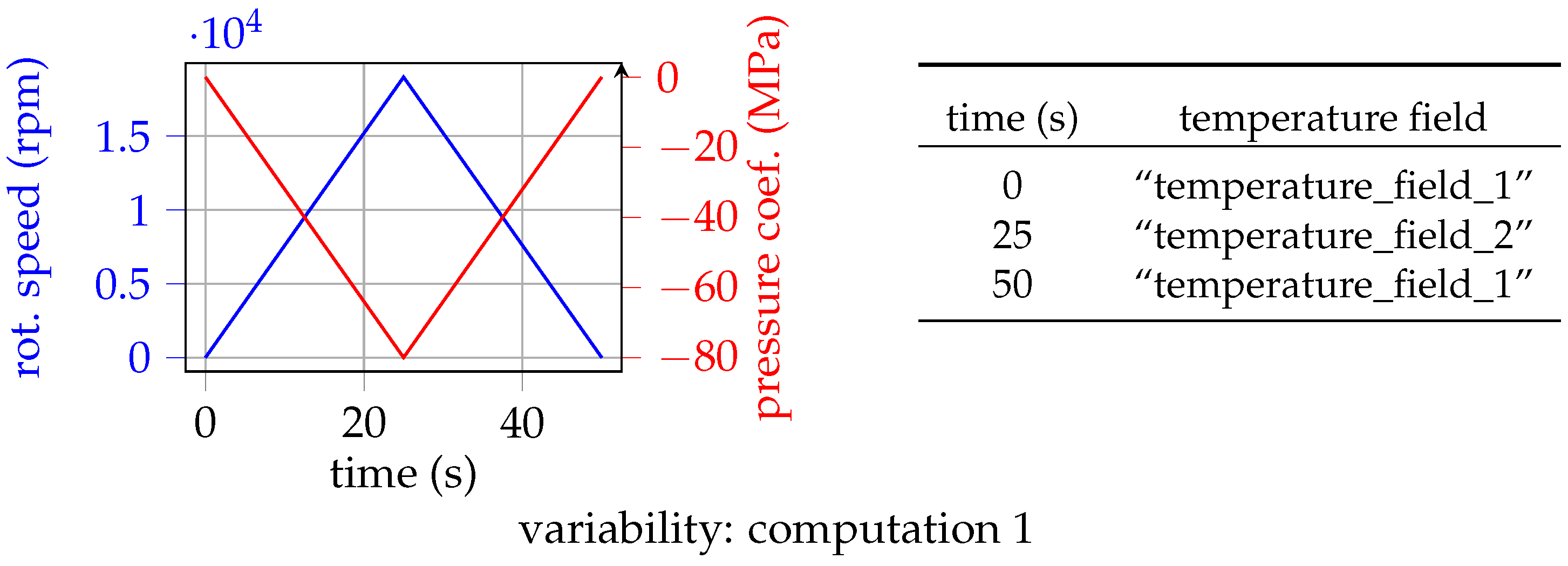
) with respect to time. (right) Temporal sequence for the temperature field.
Mca 24 00041 g007aMca 24 00041 g007b
Figure 8. Offline variability: computation 1 and computation 2; online variability: computation 1. (top) Representation of dual fields for the reference high-fidelity (HF) prediction of the online variability, the reduced order model (ROM) without enrichment, and the ROM with enrichment ((left) p at t = 50 s and (right) σ 11 at t = 25 s). (bottom) Comparison of p, σ 11 and σ 22 at the point identified by the green arrow on the top-left picture.
Mca 24 00041 g008
Figure 9. Offline variability: computation 1 and computation 2; online variability: new. (top) Representation of dual fields for the reference HF prediction of the online variability, ROM without enrichment, and ROM with enrichment ((left) p at t = 50 s and (right) σ 11 at t = 25 s). (bottom) Comparison of p, σ 11 , and σ 22 at the point identified by the green arrow on the top-left picture.
Mca 24 00041 g009
Figure 10. (left) Structure split in 48 subdomains—the top part of the blade’s material is modeled by an elastoviscoplastic law and the foot’s one by an elastic law; (right) mesh for the high-pressure turbine blade with a zoom around the cooling channels.
Mca 24 00041 g010
Figure 11. High-pressure turbine test case: (left) rotation speed with respect to time; (right) representation of maximum temperature fields used in the offline and online computations; the axis of rotation is located below the blade along the x-axis.
Mca 24 00041 g011
Figure 12. (top) Diverse HF and ROM dual quantity fields at t = 43 . 5 s for subdomain 28, (left) p, (right) σ 22 ; (bottom) comparison at the point identified by the green arrow on the top-left picture. The components of the stress tensor are in MPa.
Mca 24 00041 g012aMca 24 00041 g012b
Figure 13. (top) Diverse HF and ROM dual quantity fields at t = 43 . 5 s for subdomain 47, (left) p, (right) σ 11 ; (bottom) comparison at the point identified by the green arrow on the top-left picture. The components of the stress tensor are in MPa.
Mca 24 00041 g013
Figure 14. Complete ROM dual quantity fields at t = 43 . 5 s, with enrichment by monitoring subdomain 28. (left) Cumulated plasticity; (right) magnitude of the stress tensor.
Mca 24 00041 g014
Table 1. Characteristics for the academic test case.
number of dofs78,120
number of (quadratic) tetrahedra16,695
number of integration points81,375
number of time stepscomputation 1: 50, computation 2: 40, new: 50
behavior lawevp (Norton flow with nonlinear kinematic hardening)
Table 2. Illustration of the correlation between the reduced order model (ROM)-Gappy-proper orthogonal decomposition (POD) residual E  (13) and the error E (12) on the dual quantities cumulated plasticity p and first component of the stress tensor σ 11 .
p σ 11
computation 1 Mca 24 00041 i001 Mca 24 00041 i002
computation 2 Mca 24 00041 i003 Mca 24 00041 i004
Table 3. Comparison of the error indicator (19) with the error (12) for various offline and online variabilities, without enrichment of the reduced order model. The category “offline” for the columns refers to the variabilities used in the data generation step of the offline stage, whereas the category “online” for the rows refers to the variability considered in the online stage.
OfflineComputation 1Computation 1 and Computation 2
Online
computation 1 Mca 24 00041 i005 Mca 24 00041 i006
computation 2 Mca 24 00041 i007 Mca 24 00041 i008
new Mca 24 00041 i009 Mca 24 00041 i010
Table 4. Comparison of the error indicator (19) with the error (12) for various offline and online variabilities, with enrichment of the reduced order model.
OfflineComputation 1Computation 1 and Computation 2
Online
computation 1 Mca 24 00041 i011 Mca 24 00041 i012
computation 2 Mca 24 00041 i013 Mca 24 00041 i014
new Mca 24 00041 i015 Mca 24 00041 i016
Table 5. Characteristics for the high-pressure turbine blade test case.
number of dofs4,892,463
number of (quadratic) tetrahedra1,136,732
number of integration points5,683,660
number of time steps50
behavior law for the footelas (temperature-dependent cubic elasticity
and isotropic thermal expansion)
behavior law for the bladeevp (Norton flow with nonlinear kinematic hardening)
Table 6. Description of the computational procedure.
StepAlgorithm
Data generationAMPFETI solver in Z-set, ϵ Newton HFM = 10 - 5
Data compressionDistributed Snapshot POD, ϵ POD = 10 - 5
Operator compressionDistributed NonNegative Orthogonal Matching Pursuit, ϵ Op . comp . = 10 - 4
Reduced order model ϵ Newton ROM = 10 - 4
Dual quantities reconstructionDistributed Gappy-POD, ϵ Gappy - POD = 10 - 5
Table 7. Illustration of the correlation between the ROM-Gappy-POD residual E  (13) and the error E (12) on the dual quantities cumulated plasticity p and a component of the stress tensor σ .
p σ xx
subdomain 28 Mca 24 00041 i017 Mca 24 00041 i018
subdomain 47 Mca 24 00041 i019 Mca 24 00041 i020
Table 8. Comparison of the error indicator (19) with the error (12) for the considered offline and online variabilities. The category “plot” for the columns refers to the subdomain for which the error indicator and the error are plotted, whereas the category “enrichment” for the rows refers to the subdomain of whom the indicator is used to decide the enrichment step.
PlotSubdomain 28Subdomain 27
Enrichment
no enrichment Mca 24 00041 i021 Mca 24 00041 i022
monitoring subdomain 28 Mca 24 00041 i023 Mca 24 00041 i024
monitoring subdomain 47 Mca 24 00041 i025 Mca 24 00041 i026

