Abstract
In this paper, function approximation is utilized to establish functional series approximations to integrals. The starting point is the definition of a dual Taylor series, which is a natural extension of a Taylor series, and spline based series approximation. It is shown that a spline based series approximation to an integral yields, in general, a higher accuracy for a set order of approximation than a dual Taylor series, a Taylor series and an antiderivative series. A spline based series for an integral has many applications and indicative examples are detailed. These include a series for the exponential function, which coincides with a Padé series, new series for the logarithm function as well as new series for integral defined functions such as the Fresnel Sine integral function. It is shown that these series are more accurate and have larger regions of convergence than corresponding Taylor series. The spline based series for an integral can be used to define algorithms for highly accurate approximations for the logarithm function, the exponential function, rational numbers to a fractional power and the inverse sine, inverse cosine and inverse tangent functions. These algorithms are used to establish highly accurate approximations for and Catalan’s constant. The use of sub-intervals allows the region of convergence for an integral approximation to be extended.
Keywords:
integral approximation; function approximation; Taylor series; dual Taylor series; spline approximation; antiderivative series; exponential function; logarithm function; Fresnel sine integral; Padé series; Catalan’s constant MSC:
26A06; 26A36; 33B10; 41A15; 41A58
1. Introduction
The mathematics underpinning dynamic behaviour is of fundamental importance to modern science and technology and integration theory is foundational. The history of integration dates from early recorded history, with area calculations being prominent, e.g., [1,2]. The modern approach to integration commences with Newton and Leibniz and Thomson [3,4] provides a lucid, and up to date, perspective on the approaches of Newton, Riemann and Lebesgue and the more recent work of Henstock and Kurzweil.
A useful starting point for integration theory is the second part of the Fundamental Theorem of Calculus which states
where on [α, β] for some antiderivative function , assuming is integrable, e.g., [4,5,6]. However, within all frameworks of integration, a practical problem is to determine antiderivative functions for, or suitable analytical approximations to, specified integrals. Despite the impressive collection of results that can be found in tables books such as Gradsteyn and Ryzhik [7], the problem of determining an antiderivative function, or an approximation to the integral of a specified function, in general, is problematic. As a consequence, numerical evaluation of integrals is widely used. The problem is: For an arbitrary class of functions , and a specified interval [α, β], how to determine an analytical expression, or analytical approximation, to the integral
Approaches include use of integration by parts, e.g., [8], use of Taylor series, asymptotic expansions, e.g., [9,10], etc.
A useful approximation approach is to use uniform convergence, bounded convergence, monotone convergence or dominated convergence of a sequence of functions and a representative statement arising from dominated convergence, e.g., [11], is: If is a sequence of Lebesgue integrable functions on [α, β], pointwise almost everywhere on [α, β], and there exists a Lebesgue integrable function g on [α, β] with the property almost everywhere and for all i, then
where
For the case where is such that the corresponding sequence of antiderivative functions is known, then an analytical approximation to the integral of is defined by . It is well known that polynomial, trigonometric and orthogonal functions can be defined to approximate a specified function, e.g., [12]. In general, such approximations require knowledge of the function at a specified number of points within the approximating interval and the use of approximating functions based on points within the region of integration underpins numerical evaluation of integrals, e.g., [13]. Of interest is if function values at the end point of an interval, alone, can suffice to provide a suitable analytic approximation to a function and its integral. In this context, the use of a Taylor series approximation is one possible approach but, in general, the approximation has a limited region of convergence. The region of convergence can be extended through use of a dual Taylor series which is introduced in this paper and is based on utilizing two demarcation functions. An alternative approach consider in this paper is to use spline based approximations.
It is shown that a spline based integral approximation, based solely on function values at the interval endpoints, has a simple analytic form and, in general, better convergence that an integral approximation based on a Taylor or a dual Taylor series. Further, a spline based integral approximation leads to new series for many defined integral functions, as well as many standard functions, with, in general, better convergence than a Taylor series. The spline based series for an integral can be used to define algorithms for highly accurate approximations for specific functions and new results for definite integrals are shown. As is usual, interval sub-division leads to improved integral accuracy and high levels of precision in results can readily be obtained.
In Section 2, a brief introduction is provided for integral approximation based on an antiderivative series and a Taylor series. A natural generalization of a Taylor series is a dual Taylor series and this is defined in Section 3 along with its application to integral approximation. An alternative to a dual Taylor series approximation to a function is a spline based approximation and this is detailed in Section 4 along with its application to integral approximation. A comparison of the antiderivative, Taylor series, dual Taylor series and spline approaches for integral approximation is detailed in Section 5. It is shown that a spline based approach, in general, is superior. Applications of a spline based integral approximation are detailed in Section 6 and concluding comments are detailed in Section 7.
In terms of notation is used and all derivatives in the paper are with respect to the variable .
Mathematica has been used to generate all numerical results, graphic display of results and, where appropriate, analytical results.
2. Integral Approximation: Antiderivative Series, Taylor Series
For integral approximation over a specified interval, and based on function values at the interval endpoints, two standard results can be considered: First, an antiderivative series based on integration by parts. Second, a Taylor series expansion of an integral.
2.1. Antiderivative Series
An antiderivative series for an integral can be established by application of integration by parts, e.g., [14]: If is nth order differentiable on a closed interval [α, t] (left and right hand limits, as appropriate, at α, t) then
where
2.2. Taylor Series Integral Approximation
A Taylor series based approximation to an integral is based on a Taylor series function approximation which dates from 1715 [15]. Consider an interval [α, β] and a function whose derivatives of all orders up to, and including, exist at all points in the interval [α, β]. A nth order Taylor series of a function , and based on the point α, is defined according to
For notational simplicity, it is useful to use the latter form of the definition with the former form being implicit for the case of t = α. A Taylor series enables a function , assumed to be (n + 1)th order differentiable, to be written as
where an explicit expression for the remainder function is
See, for example, [8] or [16] for a proof. A sufficient condition for convergence of a Taylor series is for
where .
It then follows that a nth order Taylor series for the integral
based on the point , is
where
3. Dual Taylor Series
A natural generalization of a Taylor series is to use two Taylor series, based at different points, and to combine them by using appropriate weighting, or demarcation, functions. The result is a dual Taylor series.
3.1. Demarcation Functions
For the normalized case of an interval [0, 1], a dual Taylor series requires two demarcations functions, denoted and , which have the monotonic decreasing/increasing form illustrated in Figure 1. The ideal, and normalized, demarcation function are defined according to
and are such that

Figure 1.
Illustration of the normalized demarcation functions and .
Whether idealized or not, the assumption is made that and are such that (15) is satisfied. Further, for the case where is antisymmetrical around the point (1/2, 1/2), it follows that and . This is assumed.
For a dual Taylor series, the further requirement is that the demarcation functions do not affect the value of the derivatives of the series at the end points of the interval being considered. This can be achieved by the further constraints of the right and left hand derivatives, of all orders, being zero, respectively, at the points zero and one, i.e., and for .
An example of a suitable demarcation function is
and the graph of this function is shown in Figure 2 for the case of .
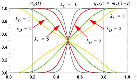
Figure 2.
Graph of the normalized demarcation functions and as defined by (16). Such functions are infinitely differentiable on (0, 1), and have right and left hand derivatives, of all orders, that are zero, respectively, at the points of zero and one.
For the denormalized case, and for the interval , the demarcation functions are defined according to
Polynomial Based Demarcation Function
Polynomial demarcation functions are of interest because, if they are associated with a Taylor series, the resulting composite function has a known antiderivative form.
A normalized polynomial based demarcation function, of order n, and for the interval [0, 1], is the (2n + 1)th order polynomial
For notational simplicity, the latter form is used with the former form being implicit for the case of t = 0. This function satisfies the constraints
and is antisymmetric around the point (1/2, 1/2). The associated quadrature polynomial demarcation function is
To derive (18), a useful approach is to solve for the coefficients of a (2n + 1)th order polynomial, subject to the constraints specified by (19), and starting with the case of . The coefficient form of in (18) can be inferred from the results specified in Pascal’s triangle.
An alternative form for is
which arises from using the binomial formula on . For notational simplicity, the latter form is used with the former form being implicit for the case of .
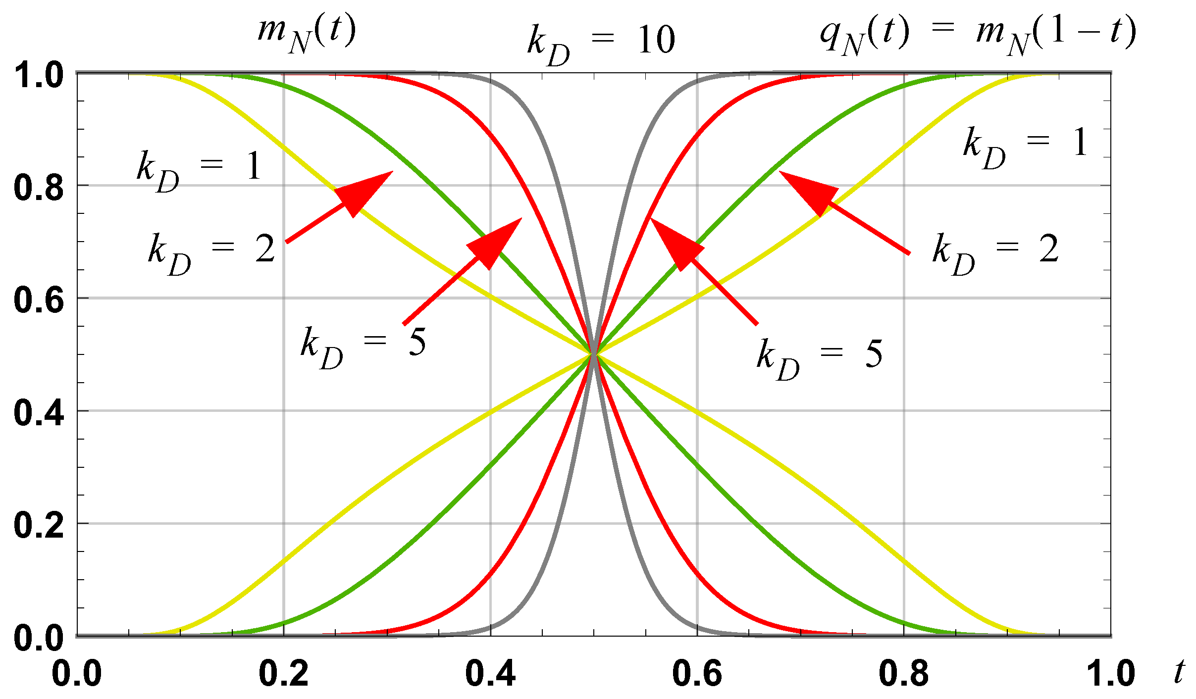
The graphs of the polynomial based demarcation functions are shown in Figure 3. For the denormalized case, and for the interval [α, β], the demarcation functions are defined according to
Explicit forms for the demarcation functions, based on the form specified in (18), are:
The second form in these equations are valid, respectively, for and , and for notational simplicity, are used.
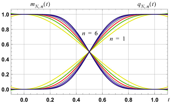
Figure 3.
Graph of the normalized polynomial demarcation functions, of orders one to six, for the interval [0, 1].
3.2. Dual Taylor Series
For the interval [α, β], a dual Taylor series, of order n, is the weighted summation of two nth order Taylor series, one based at α and one at β, and is defined according to
where m and q are the demarcation functions defined by (17). Using the Taylor series notation as specified in (7):
By construction:
For the case of polynomial demarcation functions, and , as specified by (23), and an explicit expression for is
A dual Taylor series allows a function to be written as
where the remainder function is defined according to
The proof of this result is detailed in Appendix A.
3.2.1. Convergence
With the definition of , it follows that a bound on the remainder function is
It then follows, from the nature of the demarcation functions, that a sufficient condition for the convergence of a dual Taylor series for the interval is for
For ideal demarcation functions, where the Taylor series based at only has influence on the interval [], a sufficient condition for convergence is for
3.2.2. Example
Consider the function
Dual Taylor series approximations to this function, of orders 4, 6, 8, 10, for the interval [0, 1] and defined by (27), are shown in Figure 4 using the polynomial demarcation functions specified by (23).
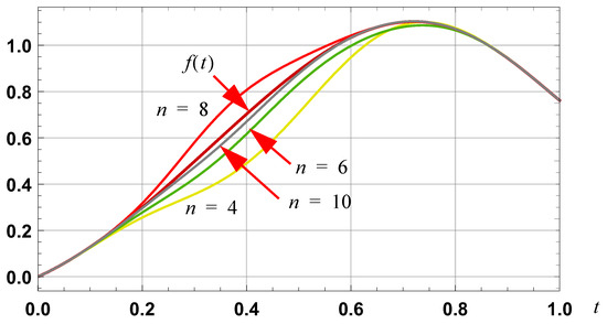
Figure 4.
Graph of the 4th, 6th, 8th and 10th order dual Taylor series approximations, based on the interval [0, 1], for the function defined by (33).
3.3. Integral Approximation
With a polynomial demarcation function, the integral of a dual Taylor series is well defined and leads to the following equality
where
and
The proof is detailed in Appendix B.
4. Spline Approximation
A nth order spline approximation, , on the interval , to a function , which is differentiable up to order , is a (2n + 1)th order polynomial that equals the function, in terms of value and derivatives up to order , at the end points of the interval. A nth order spline function for the interval , thus, has the form
where the coefficients are such that the function and the spline approximation, as well as their derivatives of order , take on the same values at the end points of the interval, i.e.,
The case of n = 1 corresponds to a cubic spline.
The use of the following symmetrical form
where and , allows the sequential solving of the unknown coefficients and leads to the result (see Appendix C):
This expression can be written in the following manner which is similar in form to that of a dual Taylor series:
where and are the denormalized polynomial demarcation functions defined by (23) and the coefficient functions are defined according to and
The proof of these results is detailed in Appendix C.
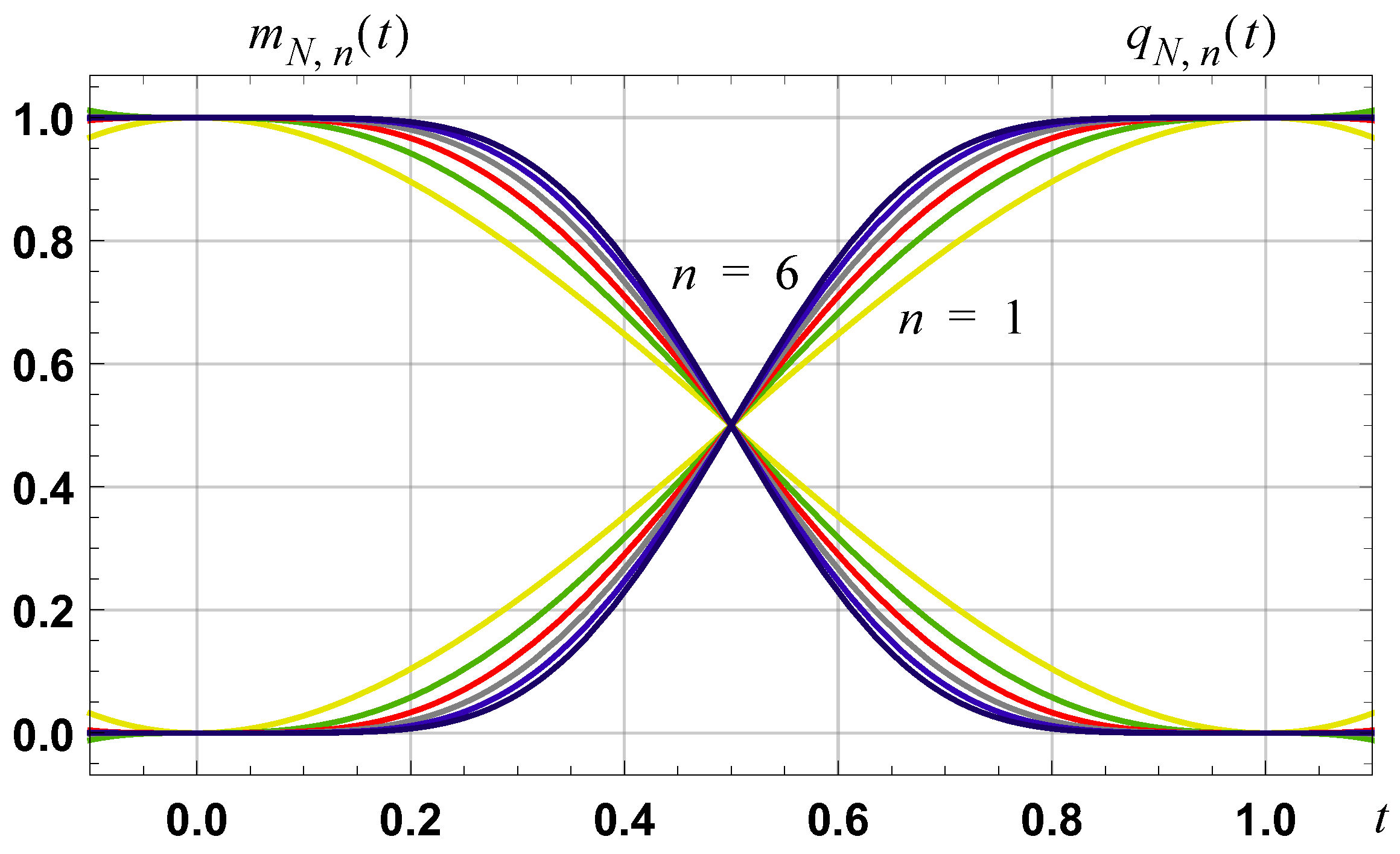
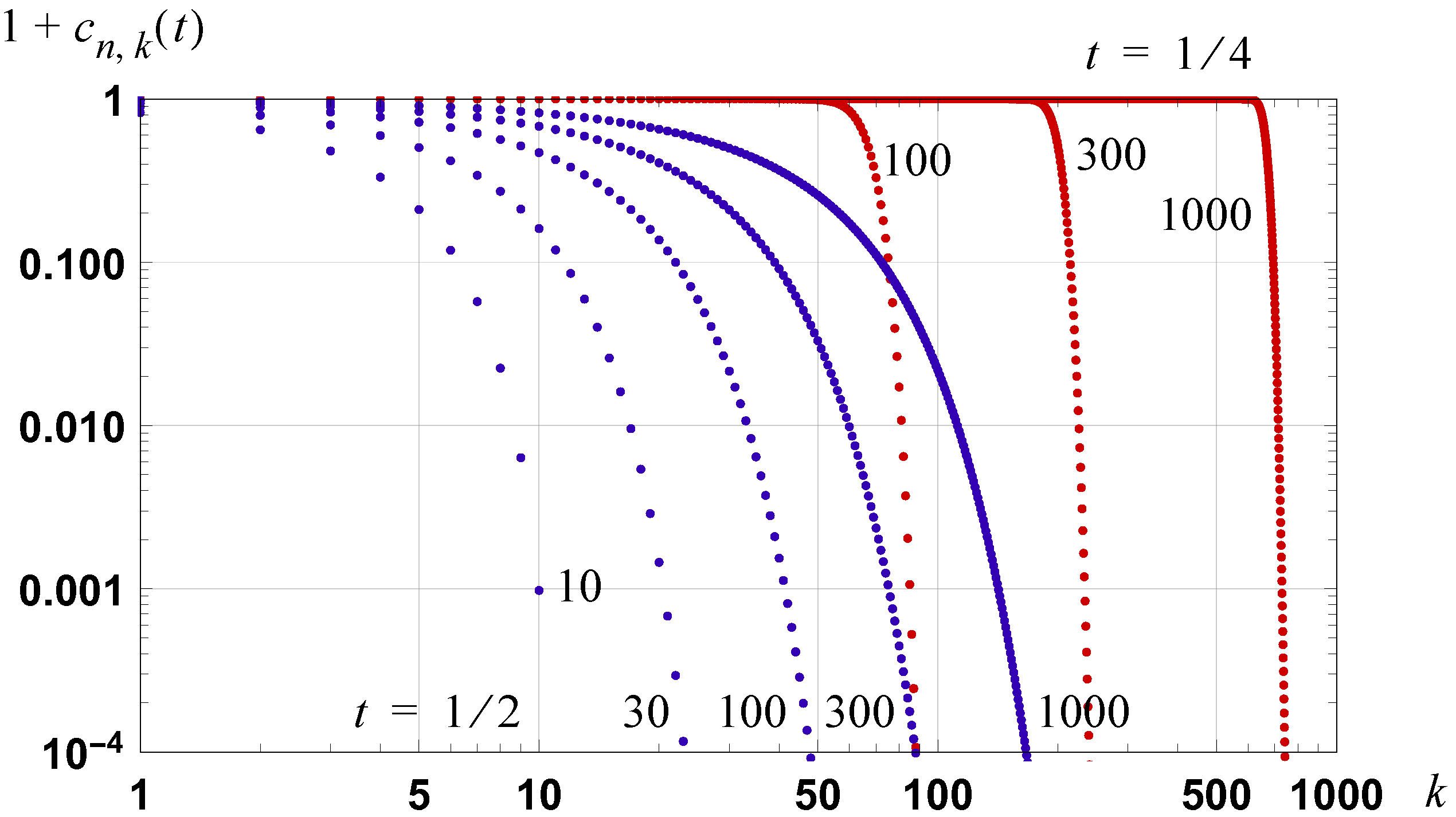
The coefficient functions are such that for and a comparison of (41) with (27) shows that a spline approximation converges to a dual Taylor approximation when and converge to zero. The variation in is illustrated in Figure 5.

Figure 5.
Graph of , for the case of and and for and . Results are shown for when and when .
4.1. Examples
The zeroth to third order spline approximations to a function for the interval are:
Spline Approximation
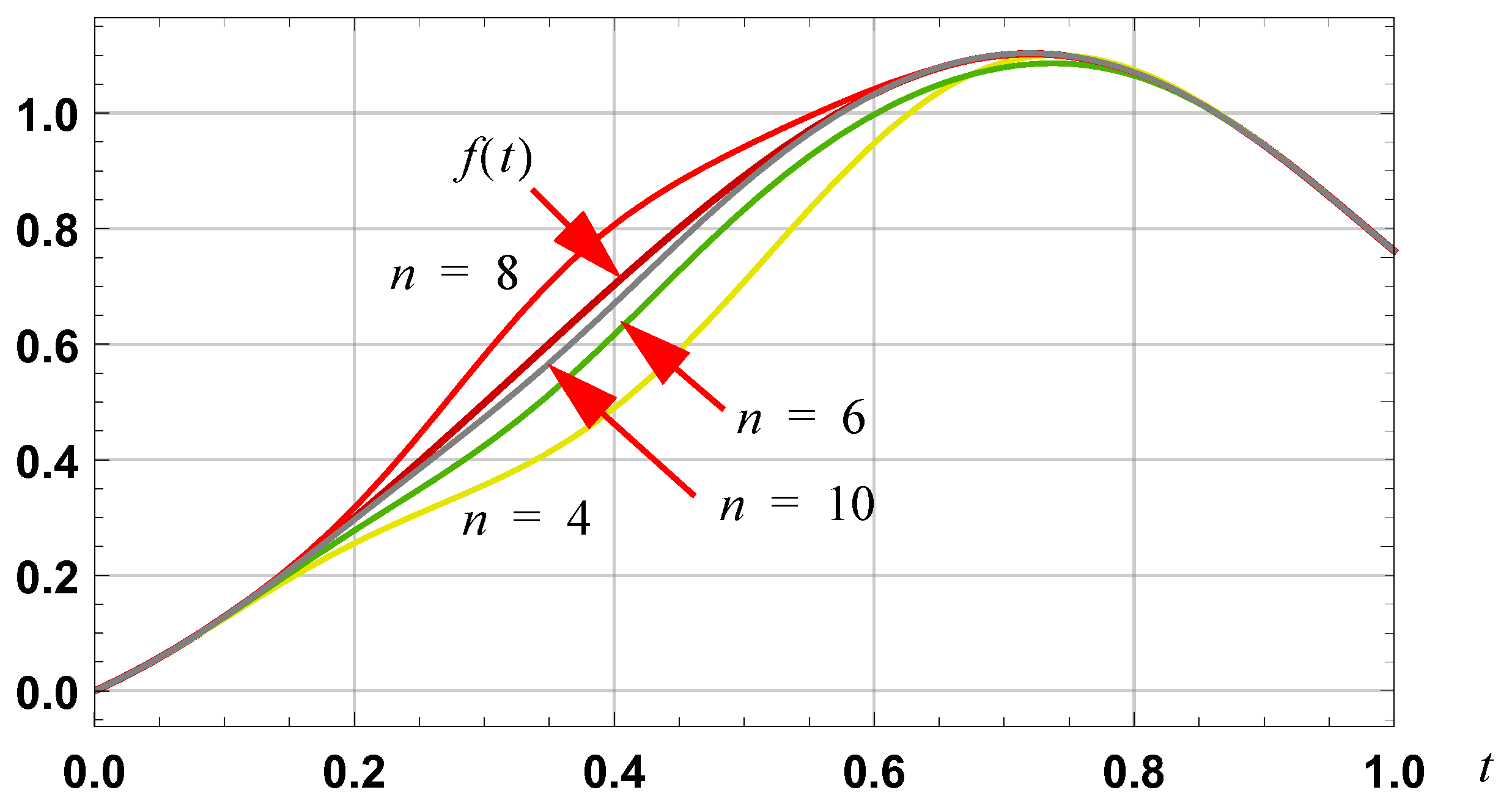
Consider the function defined by (33). Spline series approximations to this function, of orders 4, 6, 8, 10, for the interval [0, 1] and as defined by (40), are shown in Figure 6 with the 10th order approximation visually coinciding with the function. A comparison of Figure 6 with Figure 4 shows that a spline series provides, in general, a better approximation than a dual Taylor series of the same order and with a dual Taylor series diverging more in the center of the interval of approximation.
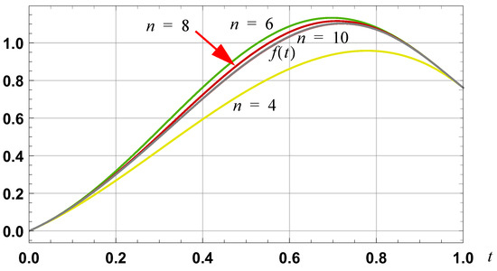
Figure 6.
Graph of 4th, 6th, 8th and 10th order spline approximations, based on the interval [0, 1], for the function defined by (33).
4.2. Convergence
Consider a spline approximation, as defined by (40) or (41). A sufficient condition for convergence, i.e., , is for
The proof of this result is detailed in Appendix D.
4.3. Spline Based Integral Approximation
The spline approximation, as defined by (40), leads to the integral equality
and the following spline based integral approximation
In these expressions the coefficients are defined according to
A simpler expression is
and this can be written, for , in the form
The remainder is defined according to
The proof of these relationships is detailed in Appendix E.
4.3.1. Approximation in Limit
It is the case that
and it then follows, for the convergent case, that
4.3.2. Integral Approximations of Orders Zero to Three
The integral approximation , as specified by (49), of orders zero to three are:
4.3.3. Remainder for Orders Zero to Three
The remainder functions associated with a spline based integral approximation, as specified according to (53), and for orders zero to three, are defined according to
4.4. Explanation of Integral Approximation: Successive Area Approximation
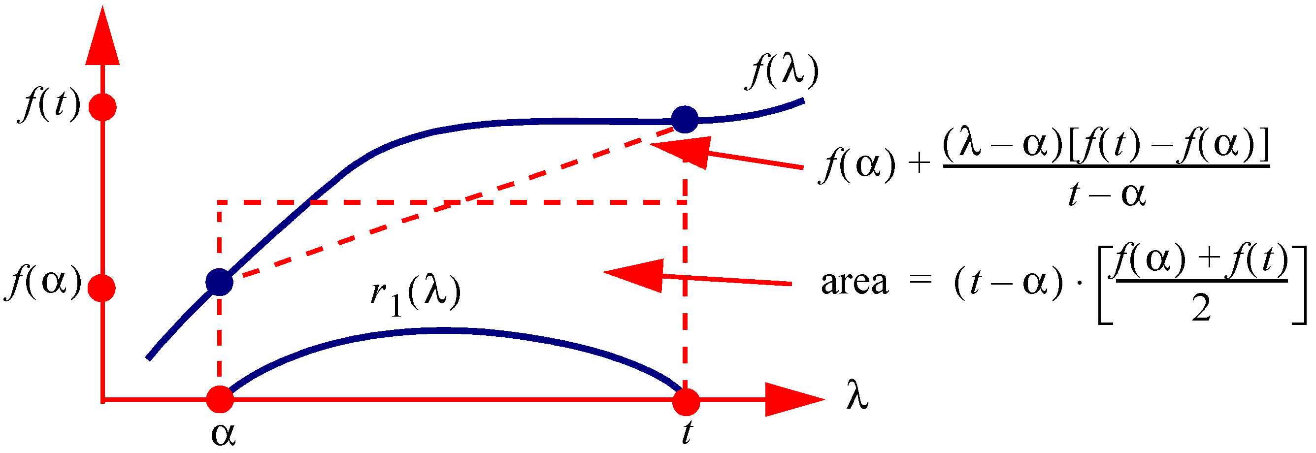
The integral approximation specified by (49), and the coefficients specified by (51), is best understood by considering successive approximations to the integral . First, consider a zeroth order approximation as defined by
and the area illustrated in Figure 7. The area is consistent with an affine approximation between the function values at the end points of the interval and equals the zeroth order integral approximation as defined by . The difference between the function and an affine approximation between the values of and defines a residual function :
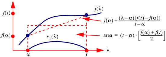
Figure 7.
Illustration of the area defined by a zeroth order approximation to an integral and the residual function .
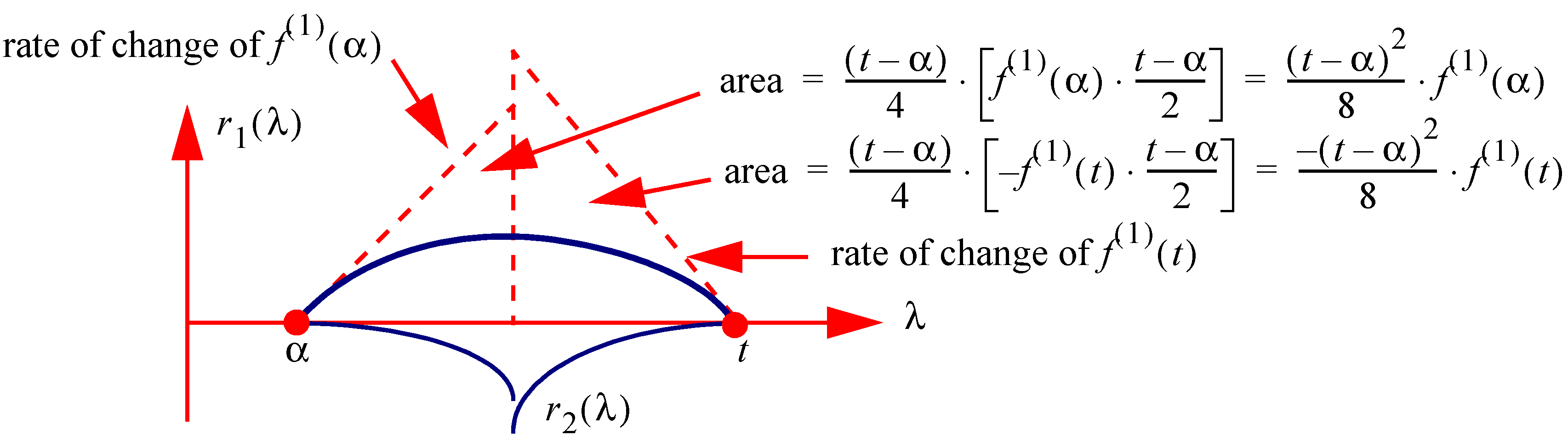
Second, consider the first order approximation to the integral as defined by
and the area illustrated in Figure 8. The second term in this equation approximates the area under an approximation to the residual function , based on linear change at both of the end points of the interval , and with a difference in the denominator terms of 12 versus 8. For higher order approximations the denominator term of 12 approaches 8.
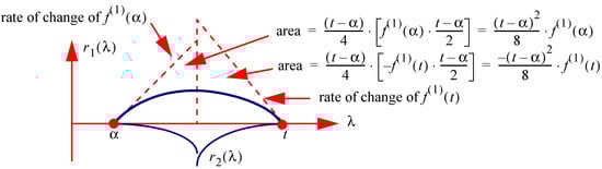
Figure 8.
Illustration of the residual function , the areas as defined by linear change at the points and t and the second residual function .
Third, consider the second order approximation to the integral as defined by
and the area illustrated in Figure 9. The third term in this expression approximates the area under a quadratic approximation to the residual function , based on and , and with a different denominator term of 120 versus 48. For higher order approximations the term of 120 approaches 48.
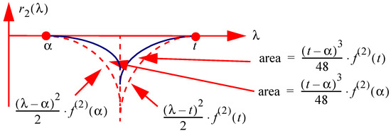
Figure 9.
Illustration of the areas defined by a quadratic approximation to the residual function and based on and .
4.5. Determining Region of Integration for a Set Error Bound
For a positive function, a bound on the region of integration, for a set error level, can be determined by considering the area defined by the first passage time of the function to a specified level. Consider a positive function, which has a first passage time to the level at , as illustrated in Figure 10. The following integral bound holds
where
Thus, for a bound on the integral of a positive function , a bound on the interval of integration is
i.e., the first passage time of to .
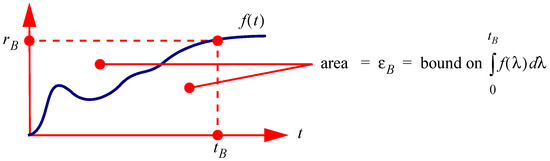
Figure 10.
The area bound defined by the first passage time of a positive function to a set level.
Consider the integral and its spline based approximation as specified by
where is specified by (53). As is known, it follows that a bound on the region of integration can be specified according to
and solved by standard root solving algorithms.
Example
Consider determining the region of integration, , for the integral and for an error bound of using the integral approximation specified by (49). The graph of is shown in Figure 11 and results are tabulated in Table 1. The specified region of integration, as expected, is conservative.
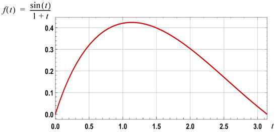
Figure 11.
Graph of over the interval [0, ].

Table 1.
Interval of integration for a spline based approximation and for a specified error bound of .
5. Summary and Comparison of Integral Approximations
The function and integral approximations detailed above are summarized in Table 2. The remainder terms associated with the integral approximations are summarized in Table 3.
Table 2.
Summary of function and integral approximations.
Table 3.
Summary of remainder terms.
Comparison of Integral Approximations
To compare the four different approximations to an integral that have been considered, and summarized in Table 2, it is useful to utilize a set of test functions. Consider a set of test functions based on a summation of Gaussian pulses
where m is an outcome of a Poisson random variable with parameter (the zero case excluded), , , are independent outcomes of random variables with a normal distribution with zero mean and unit variance, , , are independent outcomes of random variables with a uniform distribution on the interval [0, 1] and , , are independent outcomes of random variables with a uniform distribution on [0, 2]. Examples of signals are shown in Figure 12. For 1000 independently generated signals, the proportion of approximations to , with a relative error of less than 0.01, is detailed in Table 4 for the four integral approximations. The results show the clear superiority of the spline based integral approximation and simulation results for other types of signals indicate that this holds more generally.
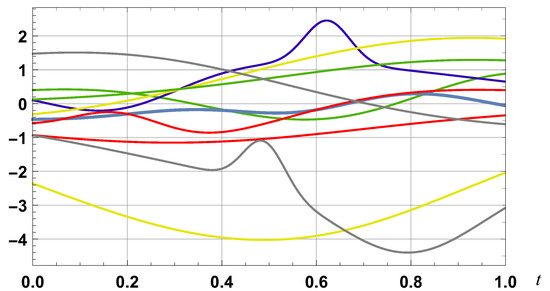
Figure 12.
Examples of test functions as defined by (73).
Table 4.
Proportion of integral approximations, based on a set of 1000 test functions, with a relative error less than 0.01.
6. Spline Based Integral Approximation: Applications
The integral based approximation, based on a nth order spline function approximation and as specified by (49), facilitates, for example, the definition of new series for standard function, new series for functions defined by integrals, and new definite integral results. In general, the series for functions have better convergence than Taylor series based approximations.
As the relative error in the evaluation of an integral, based on a spline function approximation, increases non-linearly with the region of integration, there is potential for high precision results if the value of a function defined by an integral can be established by utilizing a smaller region of integration. Several cases where this is possible are detailed.
6.1. Exponential Function Approximation
The spline based integral series, of order n, leads to the following series approximation for the exponential function
where is specified by (51). For the case of
The series converges for all . The proof of this result is detailed in Appendix F.
6.1.1. Notes
The series defined by (74) is the same as that arising from a (n + 1)th order Padé approximation, e.g., [17], which can be seen by comparing the approximations for explicit orders. A fourth order approximation (fifth order 5/5 Padé approximation) is
A direct application of the series approximation as specified by (74) is the following nth order series approximation for the Gaussian function:
6.1.2. Nature of Convergence
A nth order Taylor series approximation for exp(t), based on the origin, leads to the well known approximation
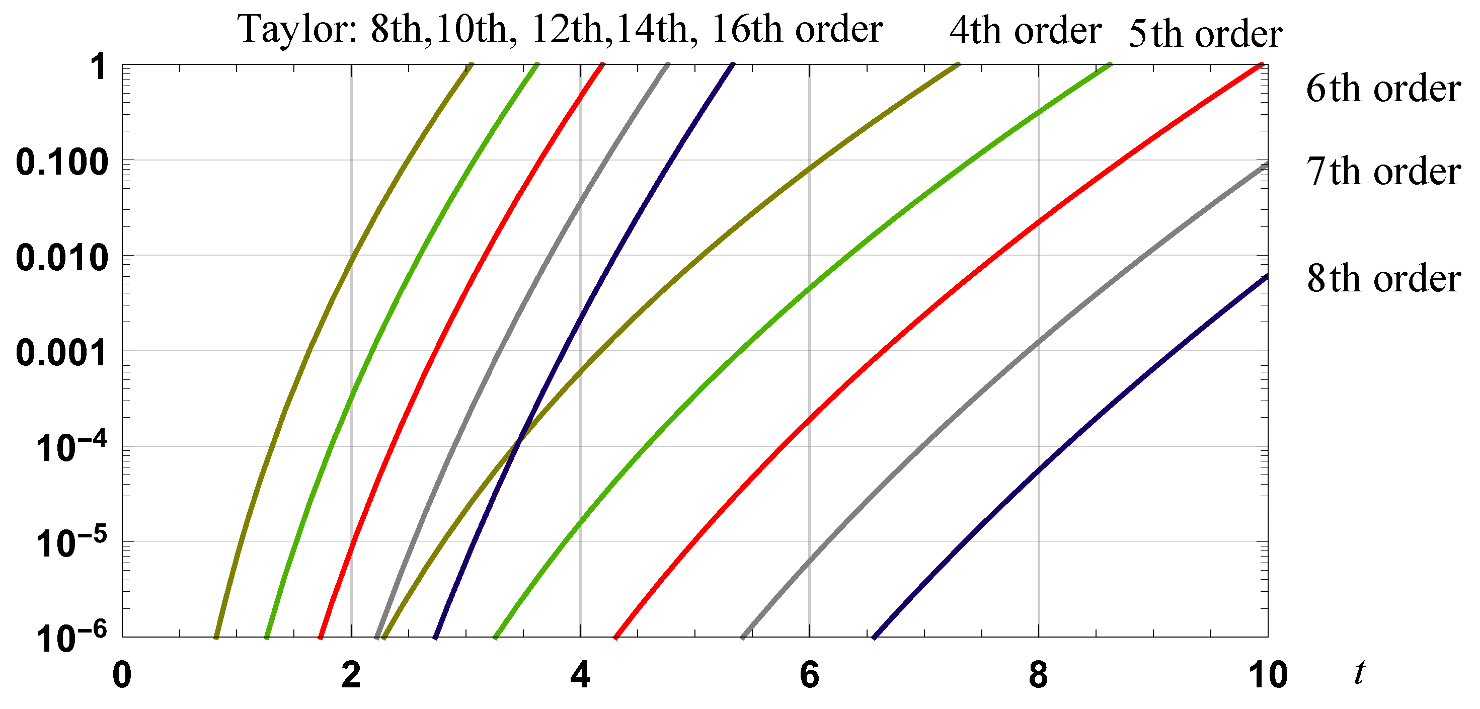
The relative error in the evaluation of exp(−t), based on this Taylor series, and the spline based series expansion defined by (74), is shown in Figure 13. The superiority of the spline based series is clearly evident.
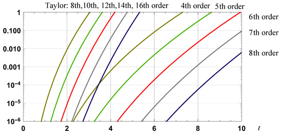
Figure 13.
Graph of the relative error in approximations to exp(−t): fourth to eighth order spline based approximations along with eighth to sixteen order Taylor series approximations.
6.1.3. High Precision Evaluation
To establish a series with a high rate of convergence consider
High precision results can be obtained as m is increased. Results that are indicative of the improvement, with increasing levels of fractional power, are detailed in Table 5 where the case of approximating e is considered.
Table 5.
Relative error in evaluation of e.
6.2. Natural Logarithm Approximation
A similar approach to that used for the exponential function leads to the following nth order series for the natural logarithm function:
where is specified by (51). The proof of this result is detailed in Appendix G.
A Taylor series, based on the point t = 1, for the natural logarithm is
The relative error in this series, and the spline based series defined by (80), is detailed in Figure 14. Simulation results indicate a region of convergence close to 0.15 < t < 6 for the spline based series-proof of a definitive bound is an unsolved problem.
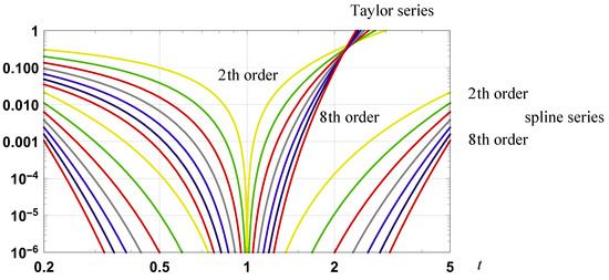
Figure 14.
Graph of the relative error in approximations to ln(t): second to eighth order Taylor series and spline based series approximation.
6.2.1. Example
A fourth order approximation is
6.2.2. High Precision Evaluation of Natural Logarithm
As the integral of ln(t) is
it follows that
Using the spline series approximation specified in (80), it follows that a nth order series approximation for ln(t), with higher precision and a greater range of convergence, is
where is specified by (51). Results that are indicative of the improvement in precision, with increasing levels of fractional power, are detailed in Table 6.
Table 6.
Relative error in evaluation of ln(t) for the case of t = 100. For the case of m = 1 the relative error is high for all orders of approximation.
6.2.3. High Precision Evaluation of ln(2)
As a second example, consider the evaluation of ln(2) which can be defined according to
One associated series, e.g., [18], p. 15, is
whilst Taylor series for ln(x), based on the points at 1 and 2, yield
i.e.,
The second series arises by finding an approximation for ln(1) based on the Taylor series at the point 2.
The relative errors in the Taylor series for orders 2, 4, 8, 16, respectively, are: 0.28, 0.16, 0.085 and 0.044 for the first series and 0.098, 0.016, 5.7 × 10⁻⁴ and 1.2 × 10⁻⁶ for the second series. The relative errors in the series defined by (87), for orders 2, 4, 8, 16, are: 0.16, 0.085, 0.044 and 0.022.
A second order series specified by (85) is
and yields an approximation with relative errors, respectively, of 1.3 × 10⁻⁴, 1.3 × 10⁻¹⁰, 1.3 × 10⁻¹⁶ and 1.3 × 10⁻²² for the cases of m = 1, 10, 100, 1000.
6.3. Evaluation of Numbers to Fractional Powers
Consider determining for the case of . With an initial approximation to of , the following integral is the basis for an iterative algorithm:
An approximation to yields an approximation for which is denoted where
Replacing by in (91) is the first step in an iterative algorithm to establish an accurate approximation to . The requirement for such an algorithm is a suitable approximation for the integral defined by and a nth order spline integral approximation is useful.
6.3.1. Iterative Algorithm
An iterative algorithm for determining an approximation to , and based on a nth order spline integral approximation, is:
where an initial number, less than , of is chosen and
Here is specified by (51). The proof of this algorithm is detailed in Appendix H.
6.3.2. Example and Results
For a 3rd order spline integral approximation, the algorithm is based on
Indicative results for the efficacy of the iterative algorithm for evaluation of a rational number to a fractional power, based on third and sixth order spline approximations, are detailed in Table 7.
Table 7.
Relative error in evaluation of for the case of , h = 6 and an initial estimate for of 9/5. .
6.4. Arc-Cosine, Arc-Sine and Arc-Tangent Function Approximation
Given the coordinate (x, y) of a point on the first quadrant of the unit circle, the corresponding angle , as defined by , and , can be determined from the following integral which is associated with the angle , :
This result is proved in Appendix I. To determine an approximation for , and, hence, , and , first, needs to be specified. Second, an approximation to the integral needs to be specified and the spline based integral approximation is efficacious.
6.4.1. Algorithm for Determining
An algorithm for determining , i ∈ {1,2,...}, is:
Here:
A direct definition for is
where an algorithm for determining is:
The proof of these results is detailed in Appendix I.
As an example, the third and fourth order functions and are:
6.4.2. Spline Based Integral Approximation
The integral defined by (97) can be approximated by using a nth order spline integral approximation as defined by (49) and (51). For the case of (x, y) specified with , approximations to , and can be determined. Based on a nth order spline integral approximation, the approximation is
where is specified by (51) and
As an example
These results arise from the spline based integral approximation as specified by (49) and (51) and by noting that
where the algorithm for determining the numerator polynomial p(k,t) is specified by (104). Substitution of this result into (49) yields
Simplification yields the result stated in (103).
6.4.3. Example and Results
With p[0, t] = 1, p[1, t] = t, p[2, t] = 1 + 2t2, p(3, t) = 3t(3 + 2t2) it follows that a third order spline based approximation is
where, for the case of i = 4, is specified in (102). The use of in (108), for the case of , yields an approximation to atan(1) = and, hence, with a relative error of 1.5 × 10⁻¹⁴. Weisstein [19] provides a good overview of approaches for calculating . Further, and indicative, results are tabulated in Table 8. High precision results can be established, for relatively low order spline based integral approximations, by using a high order of angle subdivision.
Table 8.
Relative error in approximation of based on an approximation to atan(1).
6.5. Series for Integral Defined Functions: The Fresnel Sine Integral
The spline based integral approximation, as specified by (49), can be used to define series approximations for integral defined functions. As an example, consider the Fresnel sine integral . To establish a spline based approximation for this integral the kth derivative of is required. This can be specified by using the quadrature signal and is
where
It then follows that a spline based approximation to the Fresnel sine integral is:
where is specified by (51). A sixth order approximation is
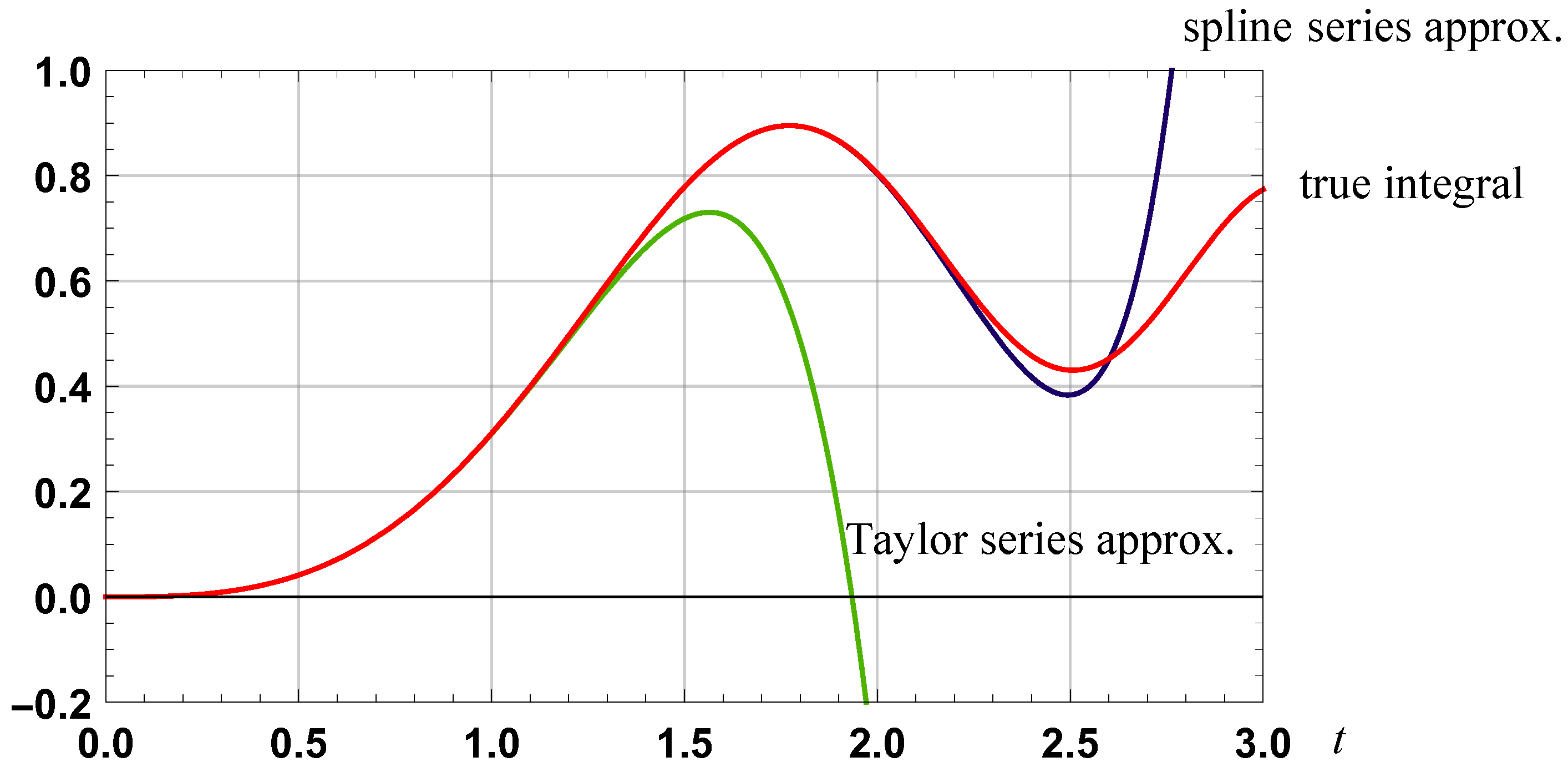
The error in a sixth order approximation to the integral is illustrated in Figure 15. The relative error is significantly less than for a standard Taylor series approximation defined, e.g., [20,21], according to
For integration over the interval [0, 1.5], the true integral is … and a 6th order spline approximation yields a relative error of −1.4 × 10⁻⁵.
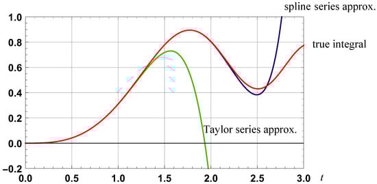
Figure 15.
Graph of approximations (order 6) to the integral of sin(t2).
6.6. Definite Integrals
The following examples illustrate the ability of spline based integral approximation to define new series for definite integrals.
6.6.1. Example 1
Consider the approximation
arising from (49), with as specified by (51), and based on the result
where , , and .
From (114), the following definite integral approximation
is valid. An alternative form is
where
A sixth order approximation is
The true value of the integral is and the relative errors in the series approximation for n = 4, 8, 16, 64, 128, 256, respectively, are 0.035, 3.3 × 10⁻³, 3.9 × 10⁻⁵, 3.2 × 10⁻¹⁶, 9.2 × 10⁻³¹ and 1.1 × 10−59.
6.6.2. Example 2: Catalan’s Constant
Consider the Catalan constant G which is defined by the series
and, equivalently, by the integral, e.g., [18], pp. 56–57,
A spline based approximation for Catalan’s constant, based on this integral, is
where is defined by (51) and
Here:
A sixth order approximation is
and has a relative error of 1.7 × 10⁻⁸. A sixth order series approximation, as specified by (120), yields an approximation with a relative error of −2.7 × 10⁻³.
6.7. Use of Sub-Division of Integration Interval
The region of convergence for a spline based integral approximation can be extended by demarcating the region of integration into sub-intervals and by using a change of variable. Consider the integral which can be written as
and can be approximated, consistent with (49) and (51), according to
where
6.7.1. Example
Consider the integral
which has the approximation detailed in (114) and where the demarcation of the interval [0, t] into m sub-intervals of measure has been used. It then follows that
where
and, based on (115),
For the case integration over the interval , the use of four subdivision intervals yields, for the case of spline based integral approximations of orders n = 4, 8, 16, 64, 128, 256, relative errors, respectively, with magnitudes of 1.0 × 10⁻⁶, 4.3 × 10⁻¹¹, 9.8 × 10⁻²⁰, 4.5 × 10−71, 2.7 × 10−139 and 1.4 × 10−275. Such results indicate the significant improvement in convergence when compared with the non-subdivision case as detailed in Section 6.6.1.
For the case integration over the interval , the use of 256 subdivision intervals yields, for the case of spline based integral approximations of orders n = 4, 8, 16, 64, 128, 256, relative errors, respectively, with magnitudes of 5.3 × 10⁻⁵, 3.3 × 10⁻⁸, 1.6 × 10⁻¹⁴, 7.5 × 10−52, 2.1 × 10−101 and 2.3 × 10−200. The true integral is .
6.7.2. Example: Electric Field Generated by a Ring of Charge
A ring in free space defined by
which has a free charge density of on it, generates an electric field at a point (x, y, z) away from the ring of
where is the permittivity of free space. As an example, consider the x component of the electric field which is defined by the integral
where
Using (127), and demarcation of into m sub-intervals of measure , this component of the electric field can be approximated according to
where
and
The algorithm for determining N(k, t) is
For example (simplification via Mathematica):
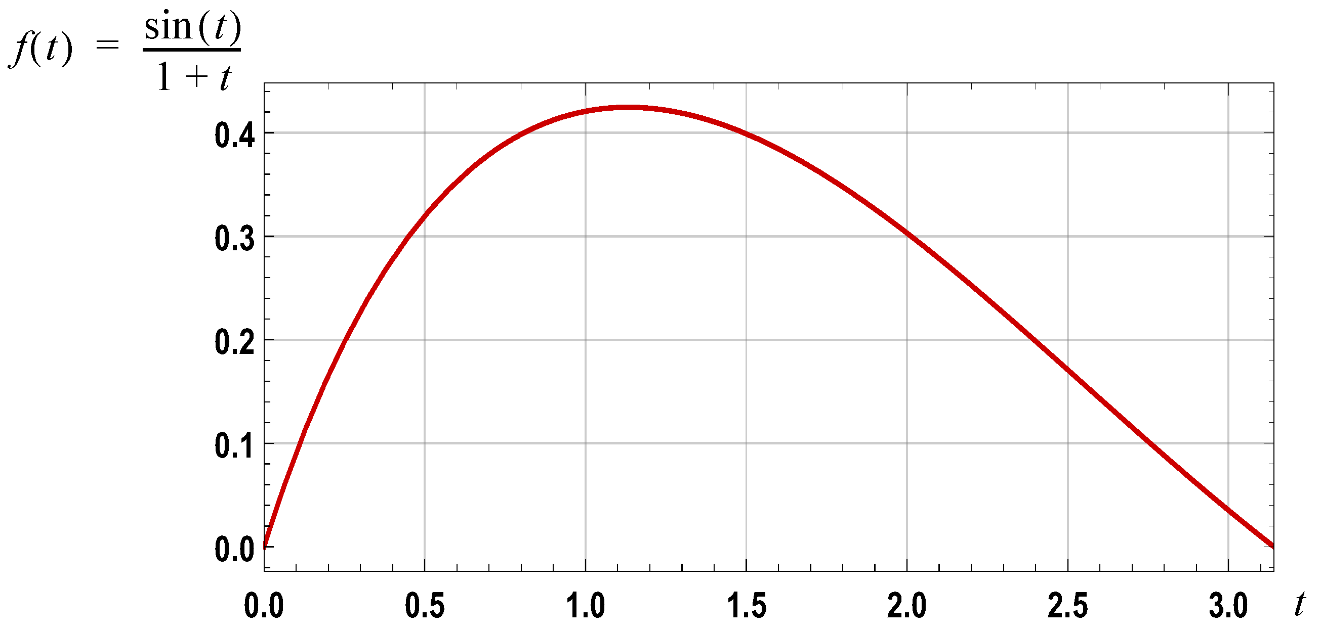
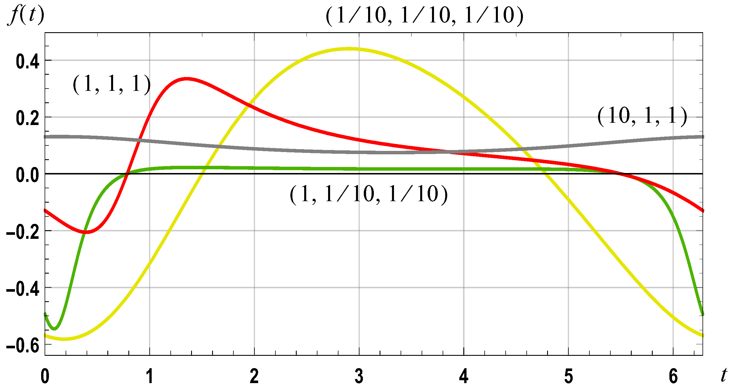
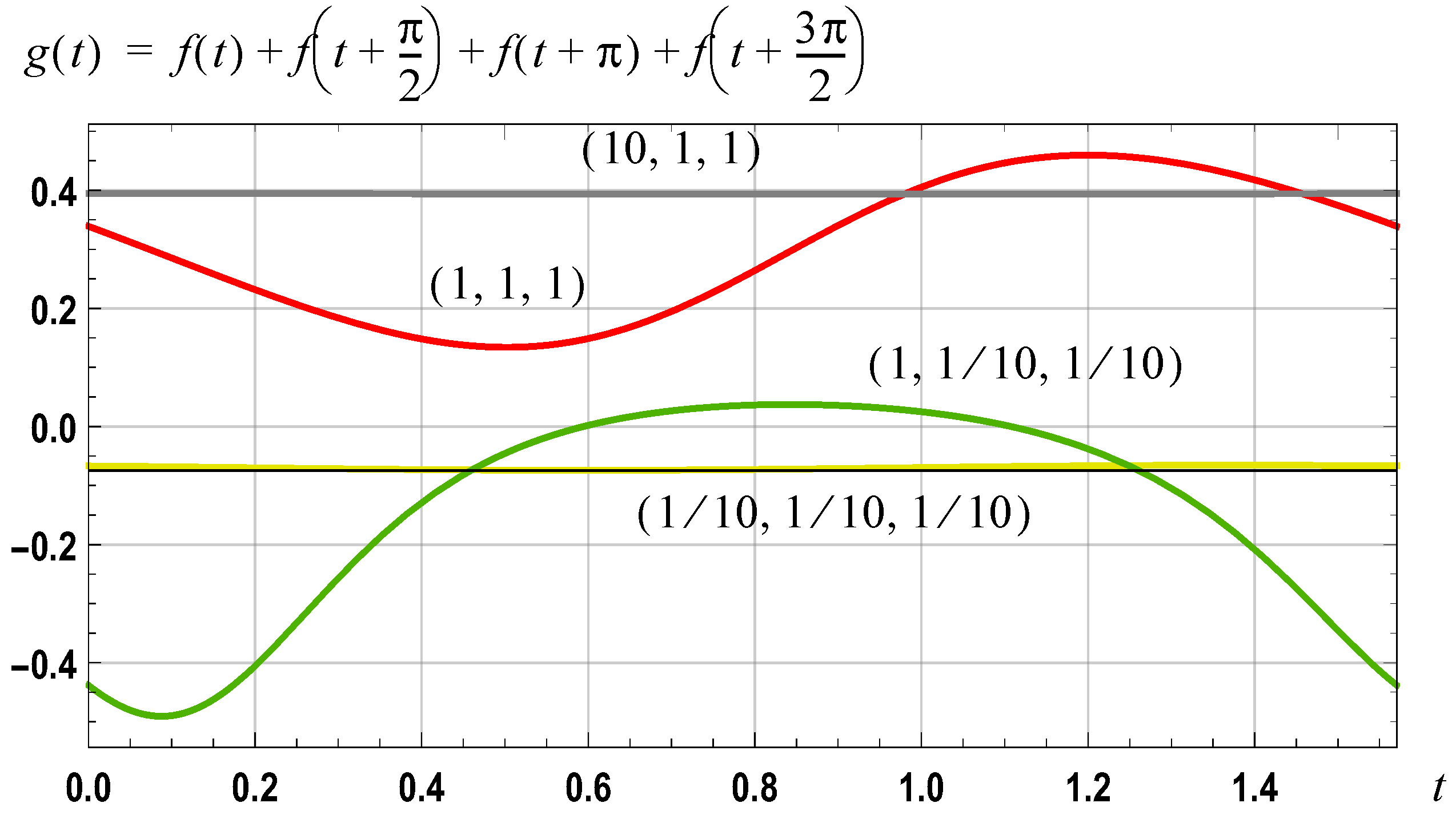
The integrand, f, varies significantly with the point (x, y, z) as is evident in Figure 16 where, for the case of a = 1 and b = 0, the graph of f is shown for the points (1/10, 1/10, 1/10), (1, 1/10, 1/10), (1, 1, 1) and (10, 1, 1). The change in the integrand with four sub-divisions of the interval is shown in Figure 17 for the same four points.
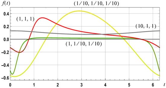
Figure 16.
Graph of f(t) for the case of a = 1, b = 0. For the case of (10, 1, 1) a scaling factor of 10 has been used; for the case of (1, 1/10, 1/10) a scaling factor of 0.1 has been used.
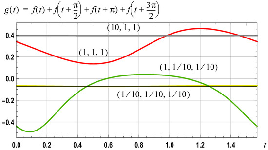
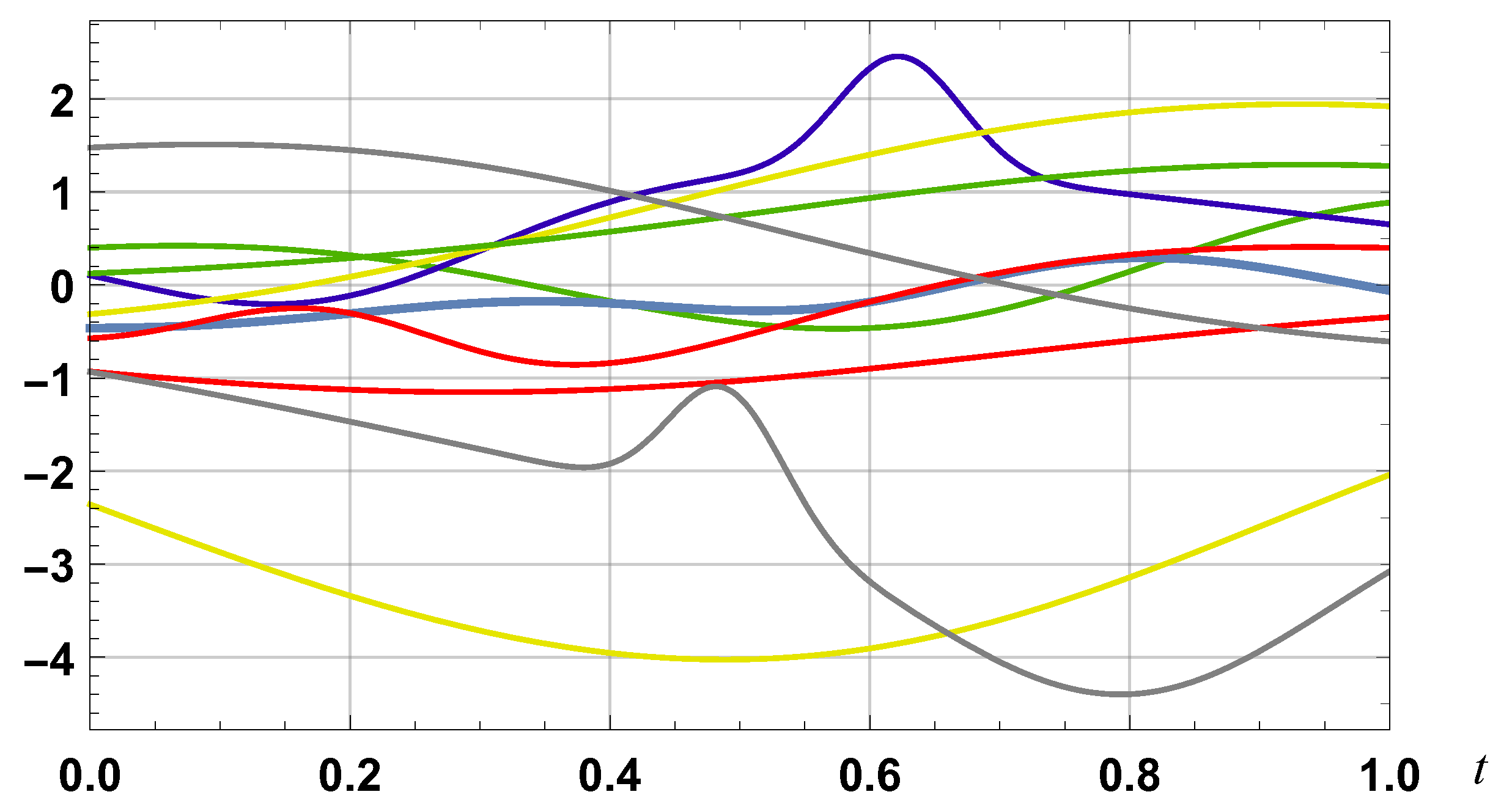
Figure 17.
Graph of g(t). For the case of (10, 1, 1) a scaling factor of 10 has been used; for the case of (1, 1/10, 1/10) a scaling factor of 0.1 has been used.
Indicative results are detailed in Table 9 and the use of four sub-intervals yields, in general, acceptable levels of error apart from the case of points close to the ring of charge where the integrand varies rapidly.
Table 9.
Magnitude of relative error in evaluation of using four sub-intervals and eight sub-intervals for the point (1, 0.1, 0.1).
7. Conclusions
This paper has introduced the dual Taylor series which is a natural generalization of the classic Taylor series. Such a series, along with a spline based series, facilitates function and integral approximation with the approximations being summarized in Table 2. In comparison with a antiderivative series, a Taylor series and a dual Taylor series, a spline based series approximation to an integral, in general, yields the highest accuracy for a set order of approximation. A spline based series for an integral has many applications and indicative examples include a series for the exponential function, which coincides with a Padé series, new series for the logarithm function as well as new series for integral defined functions such as the Fresnel Sine integral function. Such series are more accurate, and have larger regions of convergence, than Taylor series based approximations. The spline based series for an integral can be used to define algorithms for highly accurate approximations for the logarithm function, the exponential function, rational numbers to a fractional power and the inverse sine, inverse cosine and inverse tangent functions. Such algorithms can be used, for example, to establish highly accurate approximations for specific irrational numbers such as and Catalan’s constant. The use of sub-intervals allows the region of convergence for an integral to be extended. The results presented are not exhaustive and other applications remain to be found.
Acknowledgments
The support of Prof. Zoubir, SPG, Technical University of Darmstadt, Darmstadt, Germany, who hosted a visit where significant work on this paper was completed, is gratefully acknowledged. Prof. Zoubir suggested the use of a set of test functions for a comparison of the integral approximations.
Conflicts of Interest
The author declares no conflict of interest.
Appendix A. Proof of Remainder Expression for Dual Taylor Series
As for , it follows that the remainder function , as specified by (28), can be written as
Using the result for the error in a nth order Taylor series approximation, as specified in (9), i.e.,
the required results follow, namely:
Appendix B. Integral of a Dual Taylor Series with Polynomial Demarcation Functions
Consider
Substitution of and from (7), along with the definitions and for the interval , it follows, using the form specified in (21) for , that
Interchanging the order of summations and integration, and evaluation of the integrals, yields the required result:
where
The remainder is specified by
which implies
Differentiation of , and use of the result , yields the required result:
Appendix C. Proof of Spline Based Approximation
Consider the form specified by (39) for and the results:
Using these results, (39) allows the unknown coefficients to be sequentially solved. For example:
etc. Sequential solving of the equations yields the result stated in (40).
To rewrite (40) in a form that is similar to the form of a dual Taylor series, both the numerator and denominator expressions can be multiplied by for the first term, and for the second, to yield
With the definition of the polynomial demarcation functions, as specified by (23), it follows that
Adding and subtracting one from the bracketed terms, leads to the definitions for and as specified by (42) and the required form for as stated by (41).
Appendix D. Convergence of Spline Approximation
Consider the spline approximation defined by (41):
First, assume the Taylor series
converge, respectively, over the intervals and . Consistent with (32), a sufficient condition for convergence is for
It then follows that
both converge. To show this consider (42) and :
It is clear that contains one less term than in the numerator and all terms are positive. Thus, and it is the case that with equality for the case of k = 0. For n and fixed, is a monotonically decreasing series for , as is clearly evident in the graphs shown in Figure 5. It then follows, from Abel’s test for convergence [22], that the series specified in (161) are convergent.
Second, the issue is the convergence of the spline approximation to the underlying function on the interval . This follows if for as the summation is then that of a dual Taylor series. Further, and approach ideal demarcation functions as . Thus, the requirement is to prove converge of to zero for . First, using the definition of specified by (42), it can readily be shown that
and it then follows that as the first two summations comprise only of positive terms and the last double summation equals zero as the off-diagonal terms can be paired with one term being the negative of the another. Thus, for n and k fixed
when . Hence, if for , then the proof is complete. For , it is the case that the denominator term for simplifies according to
It then follows that
assuming . Hence:
Using Stirling’s formula, , yields
which clearly converges to zero as n increases for all fixed values of k. This completes the proof.
Appendix E. Proof: Integral Approximation Based on Spline Approximation
The spline based integral approximation, as specified by (49) and (50), arises from rewriting (40) in the form:
Integration of this expression over the interval then yields:
where
A change of variable yields
where B is the Beta function
As
it follows that
Substitution yields the required result:
Appendix E.1. Second Form
By directly solving for the coefficients associated with a nth order spline approximation to a function over the interval , i.e., solving for in the following approximation function
and then integrating the approximation over , yields
where the coefficients form the array:
The explicit expression can then be inferred. A direct proof of the equality between this coefficient expression and the expression implicit in (177), i.e., a direct proof of
remains elusive.
Appendix E.2. Remainder
The remainder term, specified by (53), arises from differentiation of (48) which yields
as . A change of index u = k +1 in the second summation yields
Using the definition of , as specified by (51), it follows that
and the required result follows, i.e.,
Appendix F. Proof of Series Approximation for the Exponential Function
First, the integral of the exponential function is well known, i.e.,
Second, a spline based integral approximation, as specified by (49) and (51), for the integral of the exponential function yields
Equating the right hand side of these two equations results in the required approximation
The result stated in (75), for the case of , arises from the result (54): .
The series convergence is based on the convergence of (49) for the case of an integrand of f(t) = exp(t). A sufficient condition for this is convergence of a spline based approximation for exp(t) over the interval [0, t]. Consistent with (47), a sufficient condition for this is for . On the interval [0, t], and, for t fixed:
as required.
Appendix G. Proof of Natural Logarithm Approximation
Consider the integral of ln(t):
The nth order based spline series approximation to the integral of ln(t), as defined by (49), is
where f(t) = ln(t) and , . Thus:
As , equating the right hand sides of this equation and (190) yields the approximation
Simplification yields the required result:
Appendix H. Iterative Algorithm for Number to a Fractional Power
Consider the integral result
With
where the last expression for is valid for , it follows, based on a nth order spline approximation as defined by (49) and (51), that
Here
As
it then follows that an updated approximation for is
This approximation is and is the basis for the next lower integral limit of . Thus:
Appendix I. Proof: ArcCos, ArcSin and ArcTangent Approximation
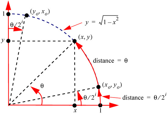
Consider a point (x, y) on the first quadrant of a unit circle, as illustrated in Figure A1, which defines an angle . The relationships , and , imply that the path length around the unit circle defined by the angle of , to the point (xo, yo), is
where
 To relate yo to x and y, consider the well known half angle results for the first quadrant:
It then follows that
and iteration leads to the algorithm:
where , , , and . It then follows that
Using the notation , it follows that
and
as required. The alternative definition for , as defined by (100), arises from a consideration of the results for ti, :
The iterative formula defined by (100) and (101) is clearly evident.
To relate yo to x and y, consider the well known half angle results for the first quadrant:
It then follows that
and iteration leads to the algorithm:
where , , , and . It then follows that
Using the notation , it follows that
and
as required. The alternative definition for , as defined by (100), arises from a consideration of the results for ti, :
The iterative formula defined by (100) and (101) is clearly evident.
Figure A1.
Geometry, based on the unit circle, for defining based on the angle .
Figure A1.
Geometry, based on the unit circle, for defining based on the angle .
References
- Burton, D.M. The History of Mathematics: An Introduction; McGraw-Hill: New York, NY, USA, 2005. [Google Scholar]
- Katz, V.J. A History of Mathematics: An Introduction; Addison–Wesley: Boston, MA, USA, 2009. [Google Scholar]
- Thomson, B.S. The natural integral on the real line. Scientiae Mathematicae Japonicae 2007, 67, 717–729. [Google Scholar]
- Thomson, B.S. Theory of the Integral. Available online: http://classicalrealanalysis.info/com/documents/toti-screen-Feb9-2013.pdf (accessed on 17 December 2018).
- Botsko, M.W. A fundamental theorem of calculus that applies to all Riemann integrable functions. Math. Mag. 1991, 64, 347–348. [Google Scholar] [CrossRef]
- Spivak, M. Calculus; Publish or Perish: Houston, TX, USA, 1994. [Google Scholar]
- Gradsteyn, I.S.; Ryzhik, I.M. Tables of Integrals, Series and Products; Academic Press: Cambridge, MA, USA, 1980. [Google Scholar]
- Horowitz, D. Tabular integration by parts. Coll. Math. J. 1990, 21, 307–311. [Google Scholar] [CrossRef]
- Olver, F.W.J. Asymptotics and Special Functions; Academic Press: Cambridge, MA, USA, 1974; Chapter 1. [Google Scholar]
- Stenger, F. The asymptotic approximation of certain integrals. SIAM J. Math. Anal. 1970, 1, 392–404. [Google Scholar] [CrossRef]
- Champeney, D.C. A Handbook of Fourier Theorems; Cambridge University Press: Cambridge, UK, 1987. [Google Scholar]
- Pinkus, A. Weierstrass and Approximation Theory. J. Approx. Theory 2000, 107, 1–66. [Google Scholar] [CrossRef]
- Davis, P.J.; Rabinowitz, P. Methods of Numerical Integration; Academic Press: Cambridge, MA, USA, 1984. [Google Scholar]
- Howard, R.M. Antiderivative series for differentiable functions. Int. J. Math. Educ. Sci. Technol. 2004, 35, 725–731. [Google Scholar] [CrossRef]
- Struik, D.J. A Source Book in Mathematics 1200–1800; Princeton University Press: Princeton, NJ, USA, 1986; pp. 328–332. [Google Scholar]
- Kountourogiannis, D.; Loya, P. A derivation of Taylor’s formula with integral remainder. Math. Mag. 2003, 76, 217–219. [Google Scholar] [CrossRef]
- Baker, G.A. Essentials of Pade Approximants; Academic Press: Cambridge, MA, USA, 1975. [Google Scholar]
- Finch, S.R. Mathematical Constants, Encyclopedia of Mathematics and its Applications; Cambridge University Press: Cambridge, UK, 2003; Volume 94, pp. 56–57. [Google Scholar]
- Weisstein, E.W. Pi Formulas, MathWorld—A Wolfram Web Resource. Available online: http://mathworld.wolfram.com/PiFormulas.html (accessed on 17 December 2018).
- Abramowitz, M.; Stegun, I.A. Handbook of Mathematical Functions with Formulas, Graphs and Mathematical Tables; Dover: Mineola, NY, USA, 1965. [Google Scholar]
- Spiegel, M.R.; Lipshutz, S.; Liu, J. Mathematical Handbook of Formulas and Tables; McGraw Hill: New York, NY, USA, 2009. [Google Scholar]
- Whittaker, E.T.; Watson, G.N. A Course of Modern Analysis; Cambridge University Press: Cambridge, UK, 1920. [Google Scholar]


© 2019 by the author. Licensee MDPI, Basel, Switzerland. This article is an open access article distributed under the terms and conditions of the Creative Commons Attribution (CC BY) license (http://creativecommons.org/licenses/by/4.0/).