Article

Thermoelastic Diffusion Multicomponent Half-Space under the Effect of Surface and Bulk Unsteady Perturbations

by
Sergey A. Davydov
1,*,
Andrei V. Zemskov
1,2 and
Elena R. Akhmetova
1
1
Moscow Aviation Institute, National Research University, Moscow 125993, Russia
2
Research Institute of Mechanics, Lomonosov Moscow State University, Moscow 119192, Russia
*
Author to whom correspondence should be addressed.
Math. Comput. Appl. 2019, 24(1), 26; https://doi.org/10.3390/mca24010026
Submission received: 2 January 2019 / Revised: 7 February 2019 / Accepted: 15 February 2019 / Published: 19 February 2019
(This article belongs to the Special Issue Mathematical Modeling in Physical Sciences)

Abstract

:
This article presents an algorithm for solving the unsteady problem of one-dimensional coupled thermoelastic diffusion perturbations propagation in a multicomponent isotropic half-space, as a result of surface and bulk external effects. One-dimensional physico-mechanical processes, in a continuum, have been described by a local-equilibrium model, which included the coupled linear equations of an elastic medium motion, heat transfer, and mass transfer. The unknown functions of displacement, temperature, and concentration increments were sought in the integral form, which was a convolution of the surface and bulk Green’s functions and external effects functions. The Laplace transform on time and the Fourier sine and cosine transforms on the coordinate were used to find the Green’s functions. The obtained Green’s functions was analyzed. Test calculations were performed on the examples of some technological processes.

1. Introduction

Creation of materials with pre-programmed properties and modification of existing materials under new quality standards is one of the development of modern areas, in the construction materials processing technological field. The mathematical model construction of the various factors impact the material being processed and the obtained result analyses allow us to consider a greater number of modification options, while minimizing financial costs in the case of complex and high-tech processes.
There are a number of approaches to mathematical model constructions. The approach to coupled fields model construction is one that is favorable, is actively developing, and gives the opportunity to most accurately and analytically describe complex dynamic technological and physical processes. An example of such a model is a thermomechanical diffusion model, which describes the interaction of temperature, displacement, and concentration fields.
The relevance of this research direction is confirmed by the presence of the large number of works in this study area, worldwide. Among the main studies, we can identify [1,2,3,4,5] as the source of the problem formulation.
Most of the currently available work are devoted to solving static [6], quasistatic [7], and stationary [8] problems of thermomechanical diffusion. However, unsteady coupled one-dimensional [9] and two-dimensional problems [10,11] are the most interesting and difficult. In these articles, the solution of the unsteady problem has been reduced to the Laplace transform on time. Its inversion is associated with great mathematical difficulties. Numerical algorithms, ready-made computational mathematics and mechanics packages have been used most often, in this case, to get the originals of the unknown functions [12]. In addition to these studies, it should be mentioned that a sufficiently detailed review on various issues of thermomechanical diffusion processes modeling for the 20th century, is available in [13]. It is important to note that the very few studies devoted to the unsteady multicomponent thermoelastic diffusion continuum.
In the represented article, we consider the one-dimensional unsteady thermoelastic diffusion problem for homogeneous isotropic multicomponent half-space. The linearized local-equilibrium model of coupled thermoelastic diffusion has been used to describe the medium perturbations propagation with finite speed. The model includes the equations of elastic medium motion, heat transfer, and mass transfer [2,4,5,14]. Initial conditions are zero.
The solution of the problem, similar to problems discussed in [15,16,17,18,19,20], is sought in the integral convolution form of Green’s functions and functions of bulk or surface external perturbations. The Laplace transform on time and the Fourier sine and cosine transform on the coordinate are used to find the Green’s functions. As a result of the transformations, the problem is reduced to a system of linear algebraic equations. Its solution is represented as rational fractions, which depend on the Laplace transform parameter. Their originals are found using well-known theorems and tables of operational calculus. Moreover, there is no need to develop new complex approaches for the numerical inversion of the Laplace transform, as it has been done in the above-mentioned works [9,10,11]. The inversion of the Fourier sine and cosine transforms, in general, can be done numerically, using such well-known approaches as the Filon’s method or the inverse Discrete Fourier Transform (DFT). Such an algorithm for the problem makes it possible to minimize the use of numerical algorithms and enables the analyses of the Green’s functions.
The unsteady problems of thermomechanical diffusion (as opposed to steady ones) make it possible to consider rapid, complex, and coupled dynamic technological processing of metals and alloys, accompanied by an explosive growth of loads and intensive mass and heat transfer [4,14,21,22]. Examples of such processes can be various pulse-periodic methods of surface treatment, such as laser [23] or electro-discharge in an oncoming liquid flow [24]. In addition to this, it is necessary to add that one of the processes that can be quite fully described by the presented mathematical model is the process of ion implantation. This technology makes it possible to obtain modified coatings, with exceptional characteristics, and create many different stable solid solutions [25,26].

2. Problem Formulation

We consider an isotropic, homogeneous, N -component half-space bounded by a surface x 1 = 0 ( O x 1 x 2 x 3 is a rectangular Cartesian coordinate system, the axis O x 1 is directed deep into the half-space). The dimensionless local equilibrium linear model of coupled thermoelastic diffusion is used to describe the medium perturbations propagation with finite speed and cross-diffusion effects [2,4,5,16,18,21]. This model includes the equation of elastic medium motion, the equation of heat transfer, and N equations of mass transfer (prime and point, respectively denotes derivatives by the dimensionless spatial variable x and by the dimensionless time τ ) [2,4,5]:
u ¨ = u b u ϑ q = 1 N α q η q + F 1 , ϑ ˙ + τ ϑ ϑ ¨ = κ ϑ b ϑ ( u ˙ + τ ϑ u ¨ ) q = 1 N β q ( η ˙ q + τ ϑ η ¨ q ) + F 2 , η ˙ q + τ q η ¨ q = p = 1 N D q p η p Λ q u M q ϑ + F q + 2 ( q = 1 ,   N ¯ ) .
Displacements, thermal, and diffusion flows are set at the boundary of the half-space [5]:
u | x = 0 = f 1 ( τ ) , ϑ | x = 0 = f 2 ( τ ) , ( Λ q u + M q ϑ p = 1 N D q p η p ) | x = 0 = f q + 2 ( τ ) .
The limitation conditions are set at infinity ( x ) [5]:
u = O ( 1 ) , ϑ = O ( 1 ) , ( Λ q u + M q ϑ p = 1 N D q p η p ) = O ( 1 ) .
Initial conditions are zero:
u | τ = 0 = u ˙ | τ = 0 = ϑ | τ = 0 = ϑ ˙ | τ = 0 = η q | τ = 0 = η ˙ q | τ = 0 0.
In Equations (1)–(4) and further, dimensionless quantities are used (if a letter coincides, then the dimensional quantity is indicated with an asterisk; q = 1 ,   N ¯ ):
x = x 1 L , τ = C t L , C 2 = C 1111 ρ , u = u 1 L , η q = n ( q ) n 0 ( q ) n 0 ( q ) , ϑ = T T 0 T 0 , D q p = D 11 ( q p ) C L , α q = α 11 ( q ) n 0 ( q ) C 1111 , Λ q = m ( q ) D 11 ( q q ) α 11 ( q ) ρ R T 0 C L , M q = D 11 ( q q ) ln [ n 0 ( q ) γ ( q ) ] C L , κ = κ 11 ρ c 0 L C , β q = n 0 ( q ) R ln [ n 0 ( q ) γ ( q ) ] m ( q ) c 0 , b u = b 11 T 0 C 1111 , b ϑ = b 11 ρ c 0 , τ ϑ = C t ϑ L , τ q = C t ( q ) L , f 1 ( τ ) = f 1 ( t ) L , f 2 ( τ ) = f 2 * ( t ) L T 0 , f q + 2 ( τ ) = f q + 2 * ( t ) n 0 ( q ) C , F 1 ( x , τ ) = F 1 * ( x 1 , t ) L C 2 , F 2 ( x , τ ) = F 2 * ( x 1 , t ) L c 0 C T 0 , F q + 2 ( x , τ ) = F q + 2 * ( x 1 , t ) L n 0 ( q ) C .
Here t is the time variable; u 1 is the displacement vector component; L is the characteristic length of half-space; q is the component number; n 0 ( q ) and n ( q ) are initial and actual concentrations (mass fractions); t ϑ is the thermal relaxation time; t ( q ) is the diffusion relaxation time; C 1111 is the elastic constant; ρ is the mass density; b 11 is a temperature constant characterizing thermal deformations; α 11 ( q ) is a coefficient characterizing the medium volumetric change due to diffusion; D 11 ( q p ) is the diffusion coefficient; m ( q ) is the molar mass; R is the universal gas constant; T 0 and T are initial and actual temperatures; κ 11 is the coefficient of thermal conductivity; γ ( q ) is the activity coefficient; c 0 is the specific heat at constant concentration and deformation; F 1 * ( x 1 , t ) is the body force; F 2 * ( x 1 , t ) is the bulk heat inflow; and F q + 2 * ( x 1 , t ) is the bulk mass inflow.

3. Integral Representation of the Solution

We present the solution of Equations (1)–(4) in the form of convolutions [15,16,17,18,19,20]:
u ( x , τ ) = k = 1 N + 2 ( G ˜ 1 k F k + G 1 k f k ) , ϑ ( x , τ ) = k = 1 N + 2 ( G ˜ 2 k F k + G 2 k f k ) , η q ( x , τ ) = k = 1 N + 2 ( G ˜ q + 2 , k F k + G q + 2 , k f k ) .
Here G ˜ i k = G ˜ i k ( x , ξ , τ ) ( i = 1 ,   N + 2 ¯ ) are the bulk and G i k = G i k ( x , τ ) are the surface Green’s functions of Equations (1)–(4) ( i = 1 ,   N + 2 ¯ ) . The convolutions have the form:
G ˜ i k F k = 0 τ d t 0 + G ˜ i k ( x , ξ , τ t ) F k ( ξ , t ) d ξ , G i k f k = 0 τ G i k ( x , τ t ) f k ( t ) d t .
Bulk Green’s functions are solutions of problems that include equations similar to system of Equation (1) [27]:
G ˜ ¨ 1 k = G ˜ 1 k b u G ˜ 2 k q = 1 N α q G ˜ q + 2 , k + δ 1 k δ ( x ξ ) δ ( τ ) , G ˜ ˙ 2 k + τ ϑ G ˜ ¨ 2 k = κ G ˜ 2 k b ϑ ( G ˜ ˙ 1 k + τ ϑ G ˜ ¨ 1 k ) q = 1 N β q ( G ˜ ˙ q + 2 , k + τ ϑ G ˜ ¨ q + 2 , k ) + δ 2 k δ ( x ξ ) δ ( τ ) , G ˜ ˙ q + 2 , k + τ q G ˜ ¨ q + 2 , k = p = 1 N D q p G ˜ q + 2 , k Λ q G ˜ 1 k M q G ˜ 2 k + δ q + 2 , k δ ( x ξ ) δ ( τ ) .
Bulk Green’s functions problem also includes zero initial conditions like Equation (4) and the following boundary conditions:
G ˜ 1 k | x = 0 = 0 , G ˜ 2 k | x = 0 = 0 , ( Λ q G ˜ 1 k + M q G ˜ 2 k p = 1 N D q p G ˜ p + 2 , k ) | x = 0 = 0 , G ˜ 1 k = O ( 1 ) , G ˜ 2 k = O ( 1 ) , ( Λ q G ˜ 1 k + M q G ˜ 2 k p = 1 N D q p G ˜ p + 2 , k ) = O ( 1 ) , x .
Here and below, δ ( x ξ ) and δ ( τ ) are the Dirac delta-function, δ k l is the Kronecker symbol.
Surface Green’s functions are solutions of problems that include homogeneous equations similar to system of Equation (1) [27]:
G ¨ 1 k = G 1 k b u G 2 k q = 1 N α q G q + 2 , k , G ˙ 2 k + τ ϑ G ¨ 2 k = κ G 2 k b ϑ ( G ˙ 1 k + τ ϑ G ¨ 1 k ) q = 1 N β q ( G ˙ q + 2 , k + τ ϑ G ¨ q + 2 , k ) , G ˙ q + 2 , k + τ q G ¨ q + 2 , k = p = 1 N D q p G p + 2 , k Λ q G 1 k M q G 2 k .
Surface Green’s functions problem also include zero initial conditions like Equation (4) and the following boundary conditions:
G 1 k | x = 0 = δ 1 k δ ( τ ) , G 2 k | x = 0 = δ 2 k δ ( τ ) , ( Λ q G 1 k + M q G 2 k p = 1 N D q p G p + 2 , k ) | x = 0 = δ q + 2 , k δ ( τ ) , G 1 k = O ( 1 ) , G 2 k = O ( 1 ) , ( Λ q G 1 k + M q G 2 k p = 1 N D q p G p + 2 , k ) = O ( 1 ) , x .
Thus, the solution of Problem (1)–(4) is reduced to finding the Green’s functions. First of all, we consider an algorithm for finding the surface Green’s functions. On the basis of this, we describe an algorithm for the bulk Green’s functions.

4. Algorithm for Finding the Surface Green’s Functions

We apply the Laplace transform on time to the homogeneous system of Equation (10) and the boundary conditions Equation (11), and get a system of differential equations [17,18,19,20] (« s » is the transformation parameter, the index « L » denotes the Laplace transformant):
s 2 G 1 k L = G 1 k L b u G 2 k L q = 1 N α q G q + 2 , k L , s ( 1 + τ ϑ s ) G 2 k L = κ G 2 k L s b ϑ ( 1 + τ ϑ s ) G 1 k L s ( 1 + τ ϑ s ) q = 1 N β q G q + 2 , k L , s ( 1 + τ q s ) G q + 2 , k L = p = 1 N D q p G p + 2 , k L Λ q G 1 k L M q G 2 k L ;
G 1 k L | x = 0 = δ 1 k , G 2 k L | x = 0 = δ 2 k , ( Λ q G 1 k L + M q G 2 k L p = 1 N D q p G p + 2 , k L ) | x = 0 = δ q + 2 , k .
Further, we apply to system of Equation (12) the Fourier sine and cosine transform (« F » denotes the Fourier transform) [28]:
G 1 k L ( x , s ) = 2 π 0 G 1 k LF ( λ , s ) sin ( λ x ) d λ , G 2 k L ( x , s ) = 2 π 0 G 2 k LF ( λ , s ) cos ( λ x ) d λ , G q + 2 , k L ( x , s ) = 2 π 0 G q + 2 , k LF ( λ , s ) cos ( λ x ) d λ .
To do this, we multiply the first equation in system of Equation (12) by sin ( λ x ) and the rest by cos ( λ x ) . Then, we integrate it along O x in the interval from 0 to + and take into account Equation (13). As a result, we obtain the system of linear algebraic equations for the Fourier–Laplace images [17,20]:
k 1 G 1 k LF b u λ G 2 k LF λ q = 1 N α q G q + 2 , k LF = λ δ 1 k , b ϑ ω λ G 1 k LF + k 2 G 2 k LF + ω q = 1 N β q G q + 2 , k LF = ( b ϑ ω δ 1 k κ δ 2 k ) , Λ q λ 3 G 1 k LF + M q λ 2 G 2 k LF χ q G q + 2 , k LF λ 2 p = 1 N D q p G p + 2 , k LF = ( Λ q λ 2 δ 1 k δ q + 2 , k ) ,
where
k 1 = s 2 + λ 2 , k 2 = ω + κ λ 2 , k q + 2 = χ q + D q q λ 2 , ω = s ( 1 + τ ϑ s ) , χ q = s ( 1 + τ q s ) .
The solution of System (15) has the form of rational fractions:
G i k LF ( λ , s ) = P i k ( λ , s ) P ( λ , s ) .
Here P ( λ , s ) is the determinant of the homogeneous System (15):
P ( λ , s ) = | k 1 b u λ α 1 λ α 2 λ α N λ b ϑ λ ω k 2 β 1 ω β 2 ω β N ω Λ 1 λ 3 M 1 λ 2 k 3 D 12 λ 2 D 1 N λ 2 Λ 2 λ 3 M 2 λ 2 D 21 λ 2 k 4 D 2 N λ 2 Λ N λ 3 M N λ 2 D N 1 λ 2 D N 2 λ 2 k N | .
P i k ( λ , s ) are the determinants obtained from P ( λ , s ) by replacing the i-th column with the right-side column of the System (15):
( λ δ 1 k , b ϑ ω δ 1 k κ δ 2 k , Λ 1 λ 2 δ 1 k δ 3 k ,     ,   Λ N λ 2 δ 1 k δ N + 2 , k ) T .
The above is done following Cramer’s rule. Below are the polynomials P i k ( λ , s ) for the two-component half-space that we will use for the calculation examples:
P 11 ( λ , s ) = λ | 1 b u α 1 α 2 b ϑ ω k 2 β 1 ω β 2 ω Λ 1 λ 2 M 1 λ 2 k 3 D 12 λ 2 Λ 2 λ 2 M 2 λ 2 D 21 λ 2 k 4 | , P 21 ( λ , s ) = ω | k 1 λ α 1 λ α 2 λ b ϑ λ b ϑ β 1 β 2 Λ 1 λ 3 Λ 1 λ 2 k 3 D 12 λ 2 Λ 2 λ 3 Λ 2 λ 2 D 21 λ 2 k 4 | , P 31 ( λ , s ) = λ 2 | k 1 b u λ λ α 2 λ b ϑ ω λ k 2 b ϑ ω β 2 ω Λ 1 λ M 1 Λ 1 D 12 Λ 2 λ 3 M 2 λ 2 Λ 2 λ 2 k 4 | , P 41 ( λ , s ) = λ 2 | k 1 b u λ α 1 λ λ b ϑ ω λ k 2 β 1 ω b ϑ ω Λ 1 λ 3 M 1 λ 2 k 3 Λ 1 λ 2 Λ 2 λ M 2 D 21 Λ 2 | , P 12 ( λ , s ) = κ λ | b u α 1 α 2 M 1 λ 2 k 3 D 12 λ 2 M 2 λ 2 D 21 λ 2 k 4 | , P 22 ( λ , s ) = κ | k 1 α 1 λ α 2 λ Λ 1 λ 3 k 3 D 12 λ 2 Λ 2 λ 3 D 21 λ 2 k 4 | , P 32 ( λ , s ) = κ λ 2 | k 1 b u λ α 2 λ Λ 1 λ M 1 D 12 Λ 2 λ 3 M 2 λ 2 k 4 | , P 42 ( λ , s ) = κ λ 2 | k 1 b u λ α 1 λ Λ 1 λ 3 M 1 λ 2 k 3 Λ 2 λ M 2 D 21 | , P 13 ( λ , s ) = λ | b u α 1 α 2 k 2 β 1 ω β 2 ω M 2 λ 2 D 21 λ 2 k 4 | , P 23 ( λ , s ) = ω | k 1 α 1 λ α 2 λ b ϑ λ β 1 β 2 Λ 2 λ 3 D 21 λ 2 k 4 | , P 33 ( λ , s ) = | k 1 b u λ α 2 λ b ϑ ω λ k 2 β 2 ω Λ 2 λ 3 M 2 λ 2 k 4 | , P 43 ( λ , s ) = λ 2 | k 1 b u λ α 1 λ b ϑ ω λ k 2 β 1 ω Λ 2 λ M 2 D 21 | , P 14 ( λ , s ) = λ | b u α 1 α 2 k 2 β 1 ω β 2 ω M 1 λ 2 k 3 D 12 λ 2 | , P 24 ( λ , s ) = ω | k 1 α 1 λ α 2 λ b ϑ λ β 1 β 2 Λ 1 λ 3 k 3 D 12 λ 2 | , P 34 ( λ , s ) = λ 2 | k 1 b u λ α 2 λ b ϑ ω λ k 2 β 2 ω Λ 1 λ M 1 D 12 | , P 44 ( λ , s ) = | k 1 b u λ α 1 λ b ϑ ω λ k 2 β 1 ω Λ 1 λ 3 M 1 λ 2 k 3 | .
Let s j = s j ( λ ) C ( j = 1 ,   2 N + 4 ¯ ) be simple zeros of the polynomial P ( λ , s ) . Based on the well-known residue theorems, the originals of the surface Green’s functions are written as follows [16,19]:
G 1 k ( x , τ ) = 2 π 0 G 1 k F ( λ , τ ) sin ( λ x ) d λ , G 2 k ( x , τ ) = 2 π 0 G 2 k F ( λ , τ ) cos ( λ x ) d λ , G q + 2 , k ( x , τ ) = 2 π 0 G q + 2 , k F ( λ , τ ) cos ( λ x ) d λ ,
where
G i k F ( λ , τ ) = j = 1 2 N + 4 P i k ( λ , s j ) P ( λ , s j ) exp ( s j τ ) .
Here prime denotes derivative by parameter « s ».
For the final expression of the unknown functions, the Green’s functions found in this way are substituted into the convolutions Equation (6). The originals in Equation (19) can be calculated using well-known numerical algorithms, such as inverse DFT-type methods or the Filon’s method. The quadrature formula on an irregular sparsening grid presented in [17] can also be used.

5. Algorithm for Finding the Bulk Green’s Functions

By analogy to the algorithm for finding the surface Green’s functions, we apply the Laplace transform on time and then the sine and cosine transform on the spatial coordinates to the inhomogeneous system of Equation (8) and boundary conditions Equation (9). Then, we get the following system of linear algebraic equations:
k 1 G ˜ 1 k LF b u λ G ˜ 2 k LF λ q = 1 N α q G ˜ q + 2 , k LF = δ 1 k sin ( λ ξ ) , b ϑ ω λ G ˜ 1 k LF + k 2 G ˜ 2 k LF + ω q = 1 N β q G ˜ q + 2 , k LF = δ 2 k cos ( λ ξ ) , Λ q λ 3 G ˜ 1 k LF + M q λ 2 G ˜ 2 k LF χ q G ˜ q + 2 , k LF λ 2 p = 1 N D q p G ˜ p + 2 , k LF = δ q + 2 , k cos ( λ ξ ) .
Its solution has the form similar to Formula (16):
G ˜ i k LF ( λ , ξ , s ) = P ˜ i k ( λ , ξ , s ) P ˜ ( λ , s ) .
Here P ˜ ( λ , s ) P ( λ , s ) is the determinant of the homogeneous system in Equation (21). P ˜ i k ( λ , ξ , s ) are the determinants obtained from Formula (17) by replacing the i-th column with the right-side column of the System (21):
( δ 1 k sin ( λ ξ ) ,   δ 2 k cos ( λ ξ ) ,   δ 3 k cos ( λ ξ ) ,   ,   δ N + 2 , k cos ( λ ξ ) ) T .
The above is done following Cramer’s rule. It is important to note that the polynomials P ˜ i k ( λ , ξ , s ) can be written through the P i k ( λ , s ) for i = 1 ,   N + 2 ¯ and k = 2 ,   N + 2 ¯ , as follows:
P ˜ i 2 ( λ , ξ , s ) = 1 κ P i 2 ( λ , s ) cos ( λ ξ ) , P ˜ i , q + 2 ( λ , ξ , s ) = P i , q + 2 ( λ , s ) cos ( λ ξ ) .
Originals of the bulk Green’s functions can be found by a method similar to system of Equation (19) and Formula (20).

6. Analysis of Singularity

In [20] it was shown that some of the surface Green’s functions originals had singularities in the form of Dirac delta functions and Heaviside functions on time, when s . If considering the finite propagation speed, there remains only one singularity of the function G 21 ( x , τ ) , in the Dirac delta function form. In the domain of Fourier–Laplace images it has the form:
lim s P 21 ( λ , s ) P ( λ , s ) = b ϑ .
This singularity can be distinguished as an integer part as follows:
P 21 ( λ , s ) P ( λ , s ) = b ϑ s 2 k 1 + P 21 * ( λ , s ) Q ( λ , s ) .
where
P 21 * ( λ , s ) = k 1 P 21 ( λ , s ) b ϑ s 2 P ( λ , s ) , Q ( λ , s ) = k 1 P ( λ , s ) .
When we substitute Equation (26) into Equation (19), the function G 21 L ( x , s ) takes the form [20]:
G 21 L ( x , s ) = 2 b ϑ π 0 s 2 k 1 cos ( λ x ) d λ + 2 π 0 P 21 * ( λ , s ) Q ( λ , s ) cos ( λ x ) d λ .
In this case, its original can be presented as follows, similar to Equation (19):
G 21 ( x , τ ) = b ϑ δ ( τ x ) + 2 π 0 G 21 F * ( λ , τ ) cos ( λ x ) d λ ,
where
G 21 F * ( λ , τ ) = j = 1 2 N + 4 P 21 * ( λ , s j ) Q ( λ , s j ) exp ( s j τ ) + 2 Re [ P 21 * ( λ , λ ) Q ( λ , λ ) ] cos ( λ τ ) 2 Im [ P 21 * ( λ , λ ) Q ( λ , λ ) ] sin ( λ τ ) .
The analysis of such singularity can help avoid errors in numerical integration and simplify the calculation of convolutions.

7. The Calculation Example on the Ion Implantation Technology

Ion implantation is a method of introducing impurity atoms into the surface of a substrate, by bombarding one with a high-energy ion beam [25,26]. As an assumption, the full cycle of ion implantation technology can be divided into several stages—the formation of the ion beam with specified characteristics, the fall of the beam on the substrate surface (target bombing process), the saturation of the target material with insertion elements and, the last stage, material annealing to form a layer of various chemical compounds and reduce internal stresses after bombing. The proposed model of thermoelastic diffusion, in a first approximation, is capable of describing the sequential stages of bombing and annealing, under the following assumptions:
  • The infinite half-space is processed evenly over the entire area.
  • Characteristics of the ion beam during the entire implantation process are constant.
  • The possible inhomogeneity of the ion beam is neglected.
  • The beam consists of only one chemical component.
  • Chemical and phase transformations are not considered.
For example, we choose the two-component problem ( N = 2 ) on the implantation of copper (Cu, q = 2 ) into an aluminum substrate (Al, q = 1 ) at the initial temperature T0 = 700 K. At the initial time, copper already has a mass fraction in the substrate medium, equal to 0.05. All the rest (0.95) is aluminum. The characteristic length of a half-space L = 10 2   m . Then, the following dimensionless values, obtained using Formula (5) [22,29,30], will correspond to the substrate medium:
M 1 = 3.00 10 14 , M 2 = 1.67 10 18 , Λ 1 = 1.17 10 16 , Λ 2 = 1.40 10 20 , D 11 = 1.37 10 15 , D 12 = 5.80 10 21 , D 21 = 4.55 10 18 , D 22 = 4.08 10 20 , α 1 = 4.41 10 9 , α 2 = 9.28 10 10 , κ = 9.65 10 7 , b u = 1.61 10 2 , b ϑ = 1.01 , τ ϑ = 127.45 , τ 1 = 1.27 10 7 , τ 2 = 6.37 10 7 , β 1 = 7.11 10 5 , β 2 = 6.98 10 6 .
We will consider the whole technological process inseparably and accept the switch time τ o = 6.37 10 6 (which corresponds to 10 3 seconds) from the implantation mode ( τ < τ o ) to the annealing mode ( τ τ o ). The switching occurs instantly.
To finalize a calculated example, we assume that the half-space boundary [25,26]
  • Is always rigidly fixed: f 1 ( τ ) 0 ;
  • At the implantation stage has no heat inflow, and at the annealing stage the heat flow is f 2 ( τ ) 4.33 10 3 H ( τ τ o ) ;
  • At the implantation stage is under inflow of Cu, but at the annealing stage mass transfer with the environment is absent: f 3 ( τ ) 0 , f 4 ( τ ) 9.87 10 12 [ H ( τ ) H ( τ τ o ) ] ;
  • Bulk and volumetric external perturbations are absent.
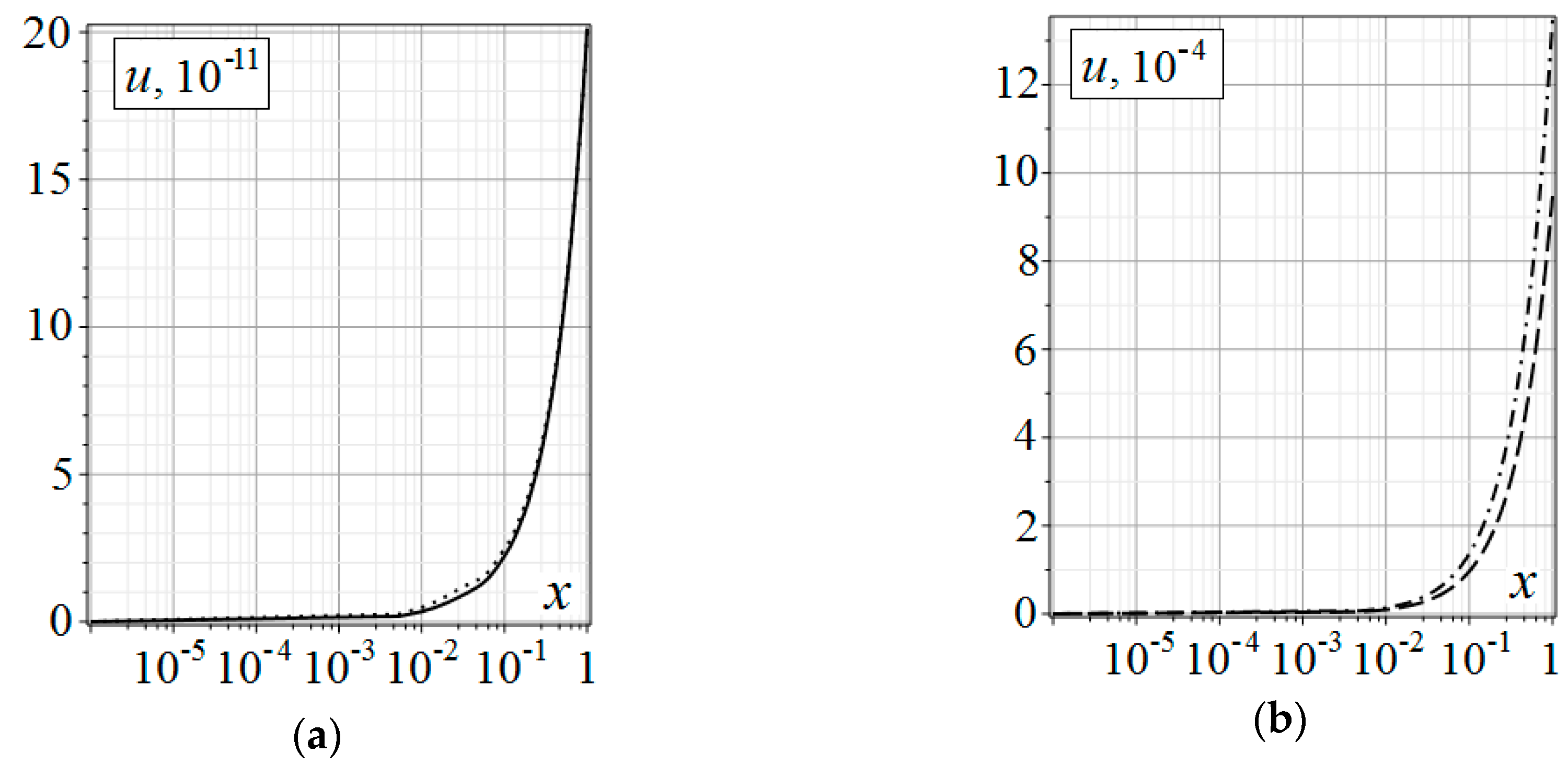
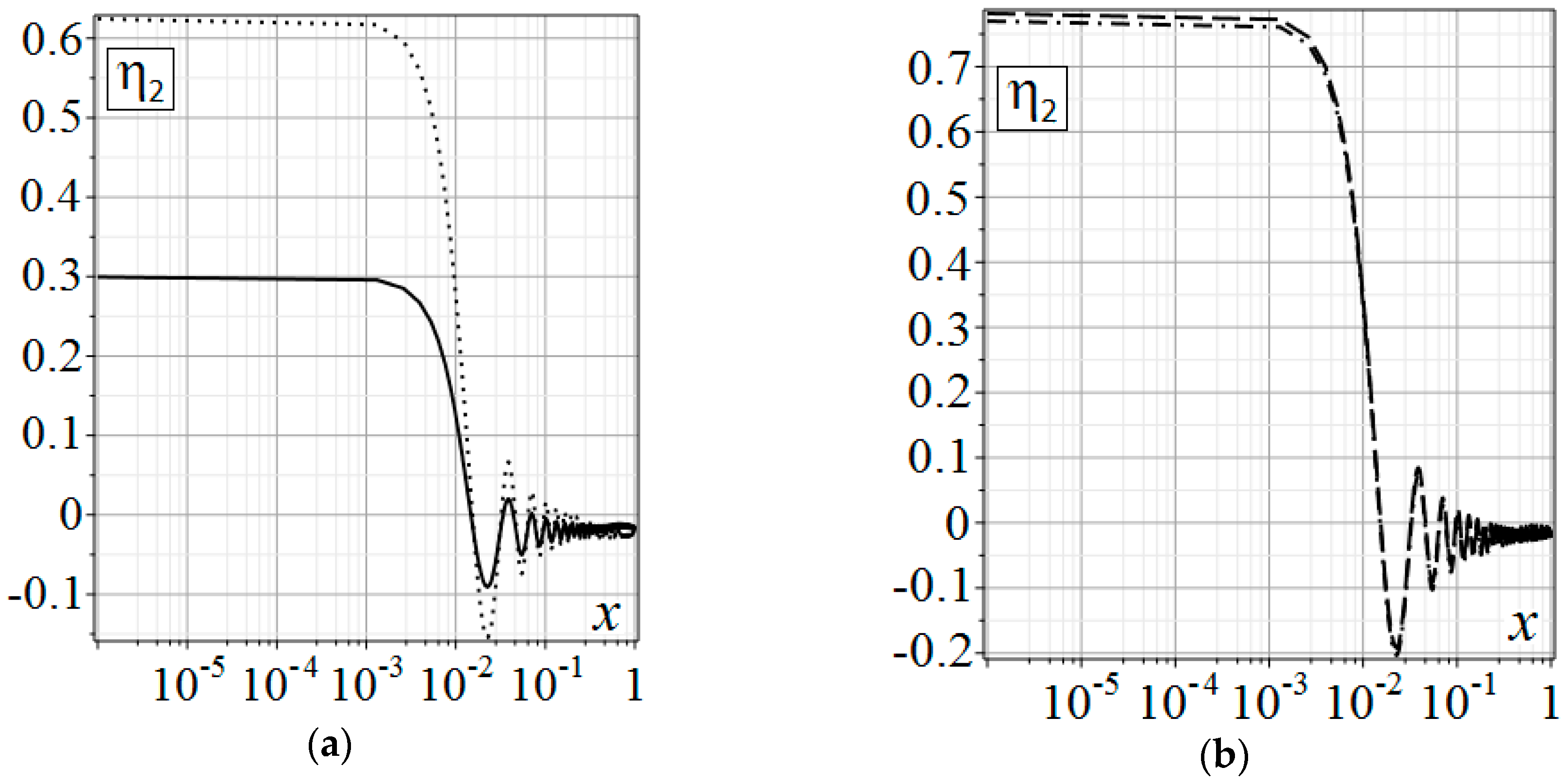
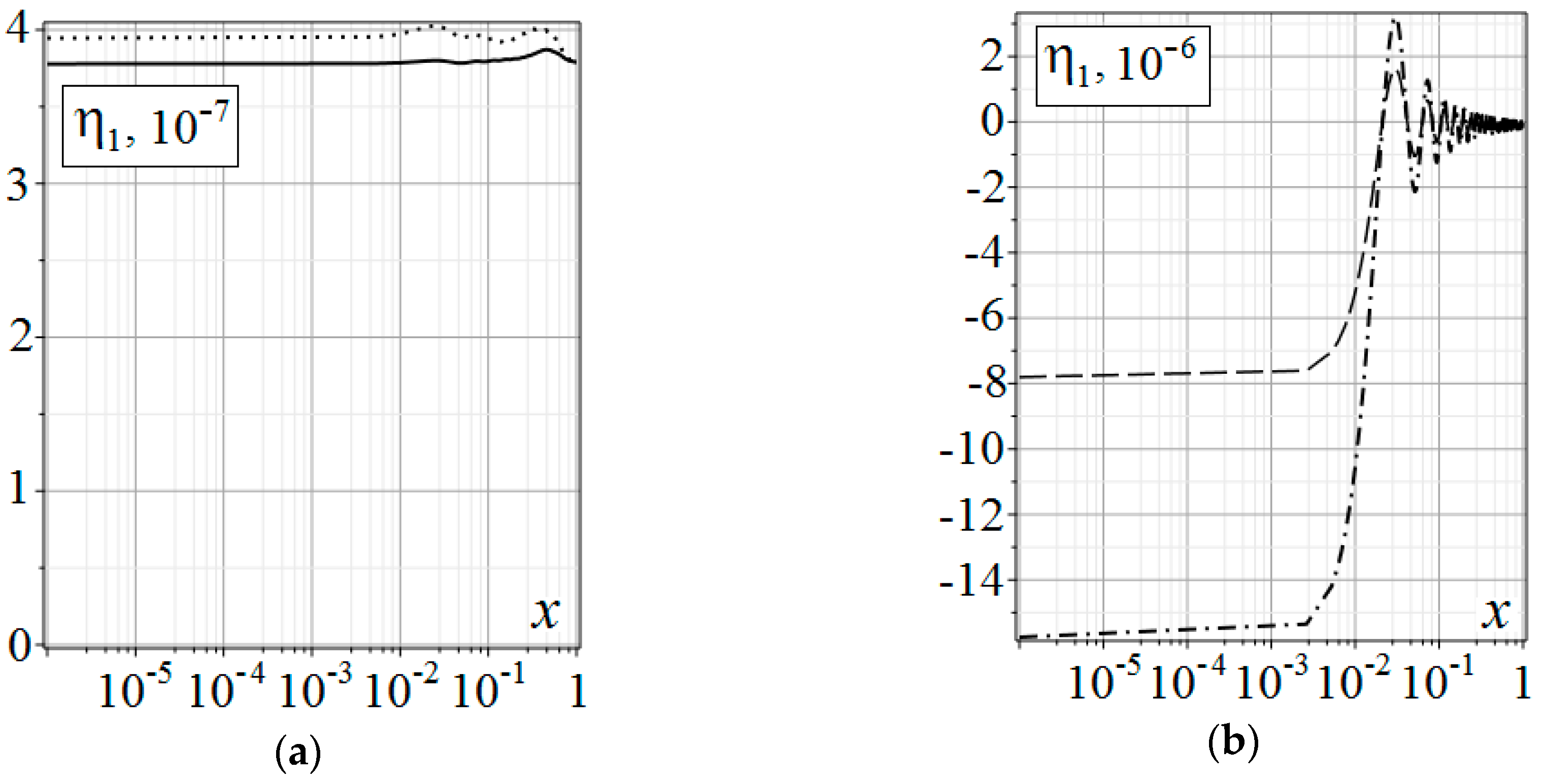
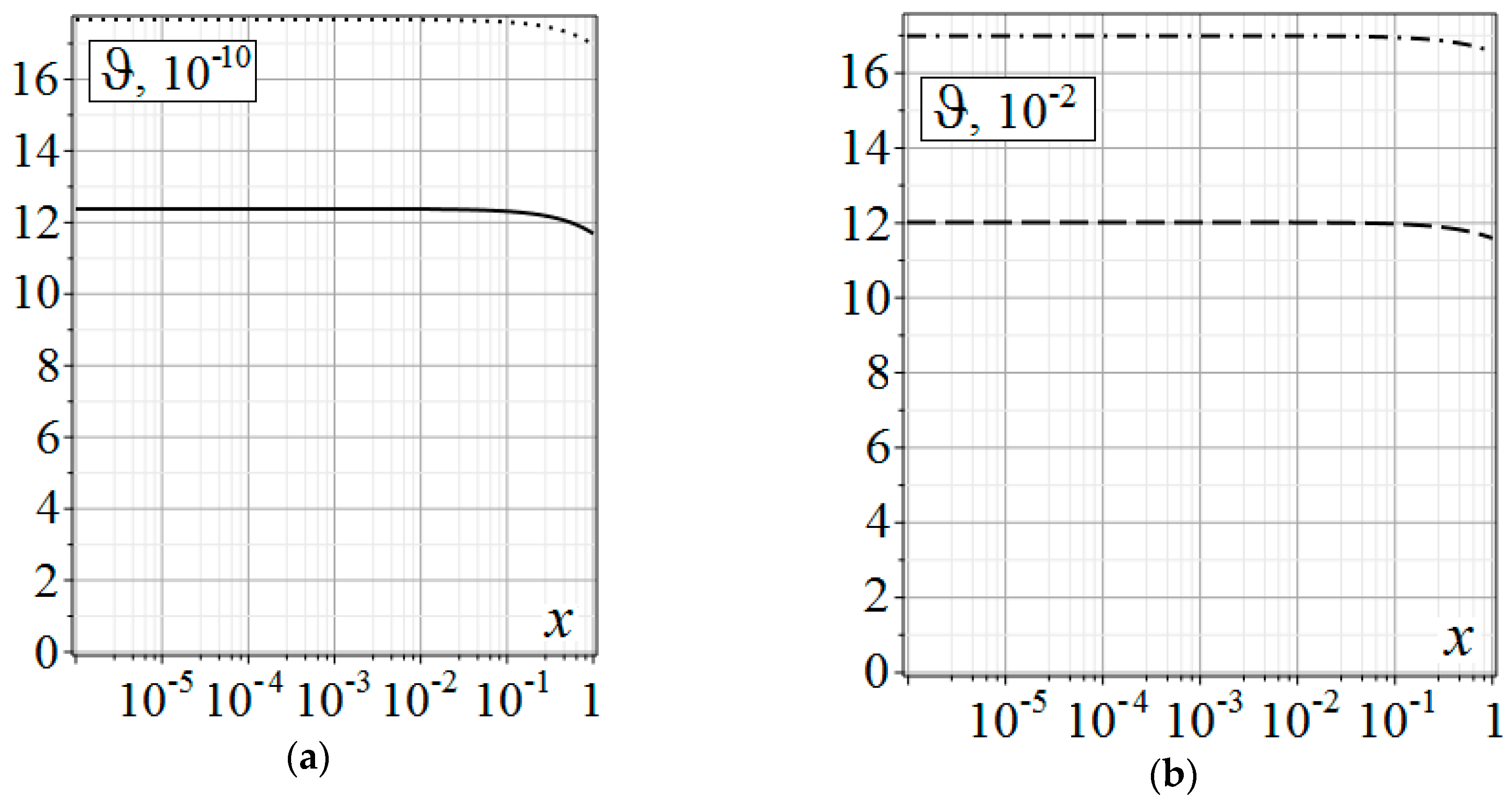
Below are the distribution graphs of thermoelastic diffusion perturbations in the medium, over depth x of the half-space. The graphs were obtained by substituting the above boundary conditions into convolution Equation (6). All convolutions were found analytical. Only the roots s j of P ( λ , s ) and the inverse sine and cosine transforms were calculated numerically. For inverse transforms we used the quadrature formula on an irregular sparsening grid [17], with 10 5 integration points. This method is quite fast, but it has a slow convergence over the grid splitting. It should be used with good convergence of the integrals in Equation (19), over the transform parameter. The left column (Figure 1a, Figure 2a, Figure 3a and Figure 4a) of the graphs shows implantation ( τ < τ o ), the right one (Figure 1b, Figure 2b, Figure 3b and Figure 4b) shows annealing ( τ τ o ).
In Figure 1, Figure 2, Figure 3 and Figure 4, τ = 0.5 τ o is indicated by the solid line; τ = 0.9 τ o is indicated by the dotted line; τ = 2 τ o is indicated by the dashed line; τ = 3 τ o is indicated by the dash-dotted line.

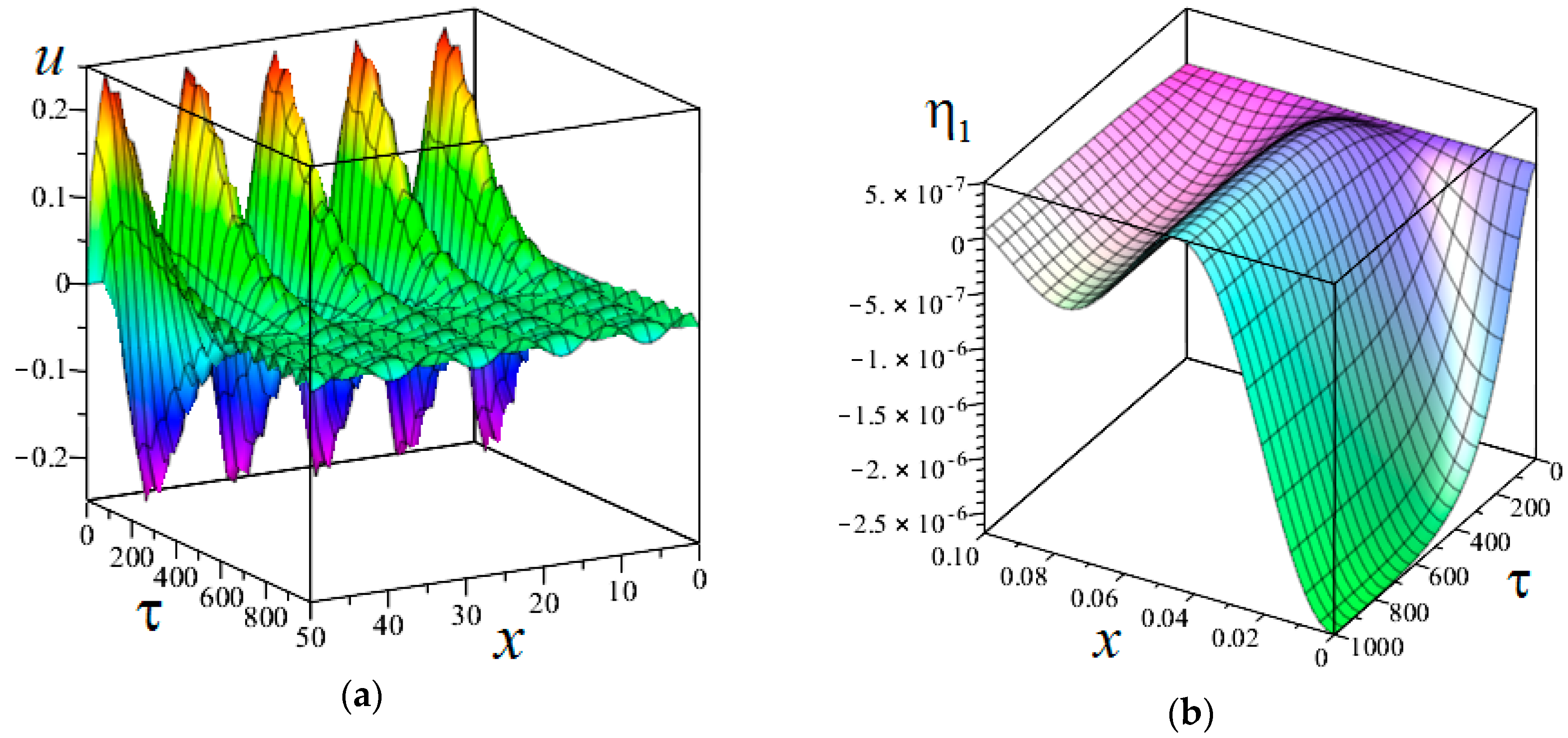
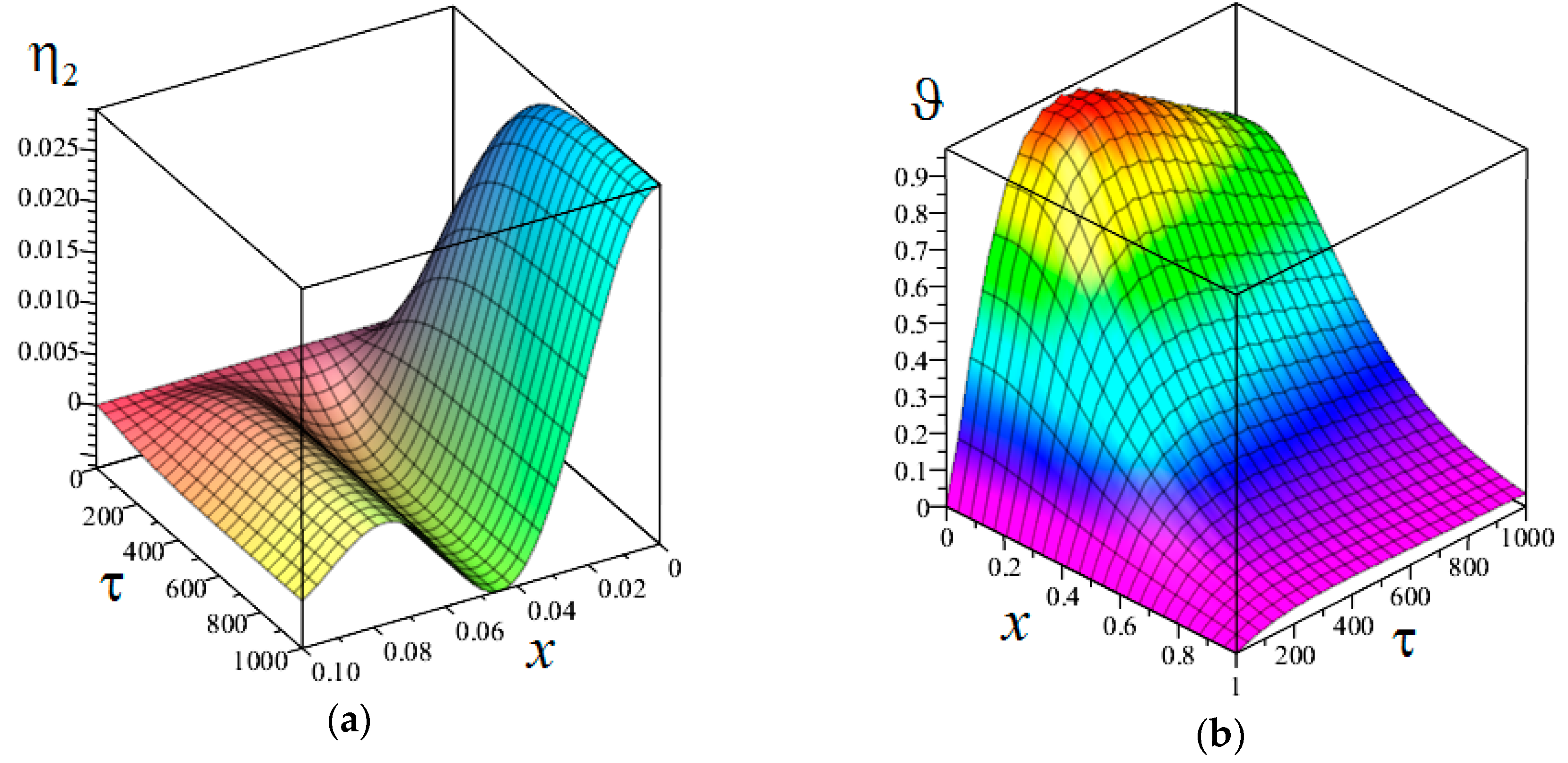
8. The Calculation Example on the Pulse-Periodic Processes

Let us consider some general pulse-periodic method of surface treatment. They can include technologies such as laser modification [23] or electro-discharge modification in an oncoming liquid flow [24]. They can be described as a first approximation of the above mathematical model, if we accept the following assumptions:
  • The infinite half-space is processed, and the impact depth is significantly less than the surface being treated.
  • A single impulse is considered.
  • Possible non-uniformity of the material is neglected.
  • Chemical and phase transformations, as well as electromagnetic fields and electron–phonon interaction are not taken into account.
For brevity and simplicity, we take the duralumin from the first calculation example with L = 10 3   m and at T 0 = 600   K :
M 1 = 3.00 10 13 , M 2 = 1.67 10 18 , Λ 1 = 1.17 10 14 , Λ 2 = 1.40 10 19 , D 11 = 1.37 10 14 , D 12 = 5.80 10 19 , D 21 = 4.55 10 16 , D 22 = 4.08 10 20 , α 1 = 4.41 10 8 , α 2 = 9.28 10 9 , κ = 9.65 10 6 , b u = 1.61 10 2 , b ϑ = 1.01 , τ ϑ = 1.27 10 3 , τ 1 = 6.37 10 5 , τ 2 = 1.27 10 6 , β 1 = 7.11 10 5 , β 2 = 6.98 10 6 .
To build the calculation example, we assume that deformations, thermal, and diffusion flows are given at the boundary of the half-space [23,24]:
f 1 ( τ ) = 3.14 10 2 τ exp ( 10 2 τ ) , f 2 ( τ ) = 2.24 10 2 τ exp ( 10 2 τ ) , f 3 ( τ ) 0 , f 4 ( τ ) = 4.93 10 8 τ exp ( 10 2 τ ) .
Of all the bulk effects, only the bulk heat inflow is set:
F 2 ( x , τ ) = 5.61 10 3 τ x exp ( 10 2 [ τ + x ] ) , F 1 ( x , τ ) 0 , F 3 ( x , τ ) 0 , F 4 ( x , τ ) 0.
Below in Figure 5 and Figure 6 are distribution graphs of thermoelastic diffusion perturbations in the half-space. The graphs were obtained by substituting the boundary conditions above into convolution Equation (6). All convolutions were found analytically. Inverse transforms were done similar to the ion implantation example. It is necessary to add that the elastic problem solution obtained using the proposed algorithm, converges with one obtained analytically.

9. Conclusions

An algorithm is proposed for solving the one-dimensional unsteady thermoelastic diffusion problem for a multicomponent half-space. The main advantage of this approach is the ability to analytically find the Laplace transform originals of the surface and bulk Green’s functions and analyze them. The originals of the Laplace transform were found analytically. It allowed us to reduce the final solution of the problem to the Fourier sine and cosine transform. The method effectiveness is demonstrated on the calculation examples technological processes.

Author Contributions

S.A.D., A.V.Z., and E.R.A. contributed equally to the writing of the main manuscript’s text and preparation of the figures. All authors reviewed the manuscript.

Funding

This work was supported by the Russian Ministry of Education and Science, Project No. 8.2118.2017/4.6.

Conflicts of Interest

The funders had no role in the design of the study; in the collection, analyses, or interpretation of data; in the writing of the manuscript, or in the decision to publish the results.

References

  1. Nowacki, W. Dynamical problems of thermodiffusion in solids. Proc. Vib. Prob. 1974, 15, 105–128. [Google Scholar]
  2. Sherief, H.H.; Hamza, F.A.; Saleh, H. The theory of generalized thermoelastic diffusion. Int. J. Eng. Sci. 2004, 42, 591–608. [Google Scholar] [CrossRef]
  3. Indeitsev, D.A.; Semenov, B.N.; Sterlin, M.D. The phenomenon of localization of diffusion process in a dynamically deformed solid. Dokl. Phys. 2012, 57, 171–173. [Google Scholar] [CrossRef]
  4. Aouadi, M.; Lazzari, B.; Nibbi, R. A theory of thermoelasticity with diffusion under Green–Naghdi models. ZAMM J. Appl. Math. Mech. 2014, 94, 837–852. [Google Scholar] [CrossRef]
  5. Knyazeva, A.G. Model of medium with diffusion and internal surfaces and some applied problems. Mater. Phys. Mech. 2004, 7, 29–36. [Google Scholar]
  6. Kumar, R.; Chawla, V. A study of Green’s functions for three-dimensional problem in thermoelastic diffusion media. Afr. J. Math. Comput. Sci. Res. 2014, 7, 68–78. [Google Scholar]
  7. Shvets, R.M. On the deformability of anisotropic viscoelastic bodies in the presence of thermodiffusion. J. Math. Sci. 1999, 97, 3830–3839. [Google Scholar] [CrossRef]
  8. Atwa, S.Y.; Egypt, Z. Generalized thermoelastic diffusion with effect of fractional parameter on plane waves temperature-dependent elastic medium. J. Mater. Chem. Eng. 2013, 1, 55–74. [Google Scholar]
  9. Salama, M.M.; Kozae, A.M.; Elsafty, M.A.; Abelaziz, S.S. A half-space problem in the theory of fractional order thermoelasticity with diffusion. Int. J. Sci. Eng. Res. 2015, 6, 358–371. [Google Scholar]
  10. El-Sayed, A.M. A two-dimensional generalized thermoelastic diffusion problem for a half-space. Math. Mech. Solids 2016, 21, 1045–1060. [Google Scholar] [CrossRef]
  11. Elhagary, M.A. A two-dimensional generalized thermoelastic diffusion problem for a half-space subjected to harmonically varying heating. Acta Mech. 2013, 224, 3057–3069. [Google Scholar] [CrossRef]
  12. Othman, M.I.A.; Elmaklizi, Y.D. 2-D problem of generalized magneto-thermoelastic diffusion, with temperature-dependent elastic moduli. J. Phys. 2013, 2, 4–11. [Google Scholar]
  13. Olesiak, Z.S. Problems of thermodiffusion of deformable solids. Mater. Sci. 1998, 34, 297–303. [Google Scholar] [CrossRef]
  14. Marin, M.; Öchsner, A. The effect of a dipolar structure on the Hölder stability in Green–Naghdi thermoelasticity. Contin. Mech. Thermodyn. 2017, 29, 1365–1374. [Google Scholar] [CrossRef]
  15. Davydov, S.A.; Zemskov, A.V.; Tarlakovskii, D.V. Surface Green’s function in non-stationary problems of thermomechanical diffusion. Prob. Strength Plast. 2017, 1, 38–47. (In Russian) [Google Scholar] [CrossRef]
  16. Tarlakovskii, D.V.; Vestyak, V.A.; Zemskov, A.V. Dynamic processes in thermoelectromagnetoelastic and thermoelastodiffusive media. In Encyclopedia of Thermal Stress; Hetnarski, R.B., Ed.; Springer: Dordrecht, The Netherlands, 2014; Volume 2, pp. 1064–1071. [Google Scholar]
  17. Davydov, S.A.; Zemskov, A.V.; Tarlakovskii, D.V. An elastic half-space under the action of one-dimensional time-dependent diffusion perturbations. Lobachevskii J. Math. 2015, 36, 503–509. [Google Scholar] [CrossRef]
  18. Davydov, S.A.; Zemskov, A.V. Unsteady one-dimensional perturbations in multicomponent thermoelastic layer with cross-diffusion effect. J. Phys. Conf. Ser. 2018, 1129, 012009. [Google Scholar] [CrossRef]
  19. Davydov, S.A.; Zemskov, A.V. Propagation of monomeric coupled thermo-elasto-diffusion disturbances in isotropic semi-space taking into account non-zero relaxation time. Trans. Krylov State Res. Cent. 2018, 2, 144–150. (In Russian) [Google Scholar] [CrossRef]
  20. Vestyak, A.V.; Davydov, S.A.; Zemskov, A.V.; Tarlakovskii, D.V. Unsteady one-dimensional problem of thermoelastic diffusion for homogeneous multicomponent medium with plane boundaries. Uchenye Zapiski Kazanskogo Universiteta (Seriya Fiziko-Matematicheskie Nauki) 2018, 160, 183–195. (In Russian) [Google Scholar]
  21. Knyazeva, A.G. Introduction to the Thermodynamics of Irreversible Processes; Ivan Fedorov Publishing House: Tomsk, Russia, 2014. [Google Scholar]
  22. Polyanin, A.D.; Vyazmin, A.V. Differential-difference heat-conduction and diffusion models and equations with a finite relaxation time. Theor. Found. Chem. Eng. 2013, 47, 217–224. [Google Scholar] [CrossRef]
  23. Adesina, O.; Popoola, P.; Fatoba, O. Laser Surface Modification—A Focus on the Wear Degradation of Titanium Alloy. Available online: http://dx.doi.org/10.5772/61737 (accessed on 15 February 2019).
  24. Akhmetova, E.R.; Tazetdinov, R.G. Titanium alloys modification for friction pairs by the method of periodic discharge in a fluid flow. Vestnik Moskovskogo Aviatsionnogo Instituta 2009, 16, 73–83. (In Russian) [Google Scholar]
  25. Ryssel, H.; Ruge, L. Ion Implantation; John Wiley & Sons Ltd.: Hoboken, NJ, USA, 1986. [Google Scholar]
  26. Goorsky, M. Ion Implantation; InTech: London, UK, 2012. [Google Scholar]
  27. Duffy, D.G. Green’s Functions with Applications; CRC Press: Boca Raton, FL, USA, 2001. [Google Scholar]
  28. Strichartz, R.S. A Guide to Distribution Theory and Fourier Transforms; CRC Press: Boca Raton, FL, USA, 1994. [Google Scholar]
  29. Grigoriev, I.S.; Meilikhov, E.Z. Handbook of Physical Quantities; CRC Press: Boca Raton, FL, USA, 1996. [Google Scholar]
  30. Szekeres, A.; Fekete, B. Continuummechanics–Heat Conduction–Cognition. Period. Polytech. Mech. Eng. 2015, 59, 8–15. [Google Scholar] [CrossRef]
Figure 1. Displacement u on x . (a) Implantation; and (b) annealing.
Mca 24 00026 g001
Figure 2. Concentration increment η 1 on x . (a) Implantation; and (b) annealing.
Mca 24 00026 g002
Figure 3. Concentration increment η 2 on x . (a) Implantation; and (b) annealing.
Mca 24 00026 g003
Figure 4. Temperature increment ϑ on x . (a) Implantation; and (b) annealing.
Mca 24 00026 g004
Figure 5. (a) Displacement u ; and (b) concentration increment η 1 .
Mca 24 00026 g005
Figure 6. (a) Concentration increment η 2 ; and (b) temperature increment ϑ .
Mca 24 00026 g006

