Article

On the Moving Trajectory of a Ball in a Viscous Liquid between Two Concentric Rigid Spheres

Moscow Aviation Institute (National Research University), Moscow 125080, Russia
*
Author to whom correspondence should be addressed.
Math. Comput. Appl. 2018, 23(4), 77; https://doi.org/10.3390/mca23040077
Submission received: 20 November 2018 / Accepted: 29 November 2018 / Published: 4 December 2018
(This article belongs to the Special Issue Mathematical Modeling in Physical Sciences)

Abstract

:
In the paper, the dynamic motion of a point ball with a mass of m , sliding in a viscous liquid between two concentric spheres under the influence of gravity and viscous and dry resistance, is investigated. In addition, it is considered that the ball starts its motion from some arbitrary point M 0 = M ( θ 0 , φ 0 ) . A system of nonlinear differential equations in a spheroidal coordinate system is obtained for the angular variables θ and φ to account for all the forces acting on the ball. The dependence of the reaction force on the angular variables is found, and the solution of the resulting system of equations is numerically analyzed. The projections of the trajectories on the plane x y ,   y z ,   x z are found.

1. Introduction

The problem which is considered in this paper belongs to the category of problems of classical mechanics. The work presented in this paper is devoted to the derivation of a system of dynamic equations describing the trajectory of the complex motion of a ball of arbitrary size moving between two concentric spheres of radiuses R 1 and R 2 . They are satisfying the simple relation R 2 = R 1 + d , where d is the diameter of the ball with a mass of m . The problem we are considering in this paper intersects somewhat with the problem described in the monograph [1] on a spherical pendulum.
However, the abovementioned problem concerns the description of the motion of a ball between spherical surfaces, and the solution of the problem itself is not given. In a previous paper [2], a spherical pendulum is considered with allowance for viscous friction only and the equations without an exact decision are given. In this paper, we are filling in the missing components and giving a pure analytical solution for the problem posed, but in the more complicated case, when the ball moves between two concentric spheres, taking into account both the viscous and dry frictions.

2. The Solution of the Problem

We suppose that the interval between the concentric spheres is filled by a viscous continuum with a dynamical viscosity η , and 
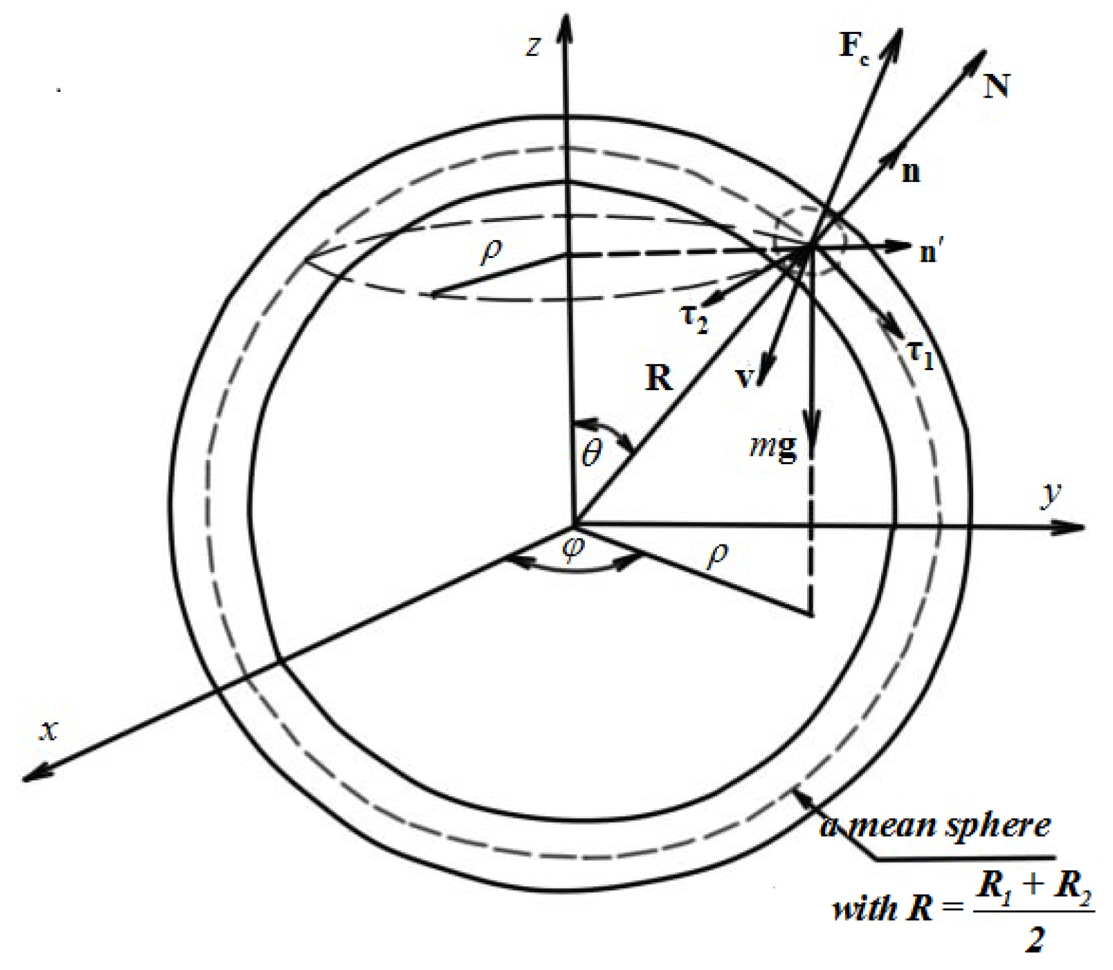
Figure 1 shows the geometry of the problem.
Since the ball has an arbitrary size, we cannot neglect its diameter in comparison with the radiuses of R 1 and R 2 . It means that we need to introduce the element of the metric on the surface due to the middle radius of the sphere R = R 1 + R 2 2 , i.e.,
d l 2 = R 2 d θ 2 + R 2 sin 2 θ d φ 2 .
Hence, the velocity of the ball can be represented in the next form
v 2 = R 2 θ ˙ 2 + R 2 sin 2 θ φ ˙ 2 .
In the instantaneous unit basis at the surface of the middle sphere of τ 1 and τ 2 , for the velocity, we have
v = v θ τ 1 + v φ τ 2 ,
where the velocity components are
v θ = R θ ˙ ,   v φ = R sin θ φ ˙
Differentiating Equation (3) in order to find the following equation for the complex acceleration of the ball gives:
a = R θ ¨ τ 1 + R θ ˙ τ ˙ 1 + R θ ˙ φ ˙ cos θ τ 2 + R sin θ φ ¨ τ 2 + R φ ˙ sin θ τ ˙ 2 ,
where τ ˙ 1 = d τ 1 d l 1 d l 1 d t = v θ n R = θ ˙ n , τ ˙ 2 = d τ 2 d l 2 v φ = R sin θ φ ˙ n R sin θ = φ ˙ n ; n —a normal unit vector, where n = n 1 n 2 2 ; and n is directed along the circle radius ρ = R sin θ and n lies in the plane of the unit vectors of τ 1 , n . In the result, we thus obtain the following for the complex acceleration:
a = R θ ¨ τ 1 + R θ ˙ 2 n + R θ ˙ φ ˙ cos θ τ 2 + R sin θ φ ¨ τ 2 + R φ ˙ 2 sin θ n
It means that we can write the equation of the motion in a general form as
a = g + N n m + F c m ,
where N is the resulting reaction force between the outer and inner spheres. We use this in the next correlation N n = N 1 n 1 N 2 n 2 2 , where N 1 is the reaction force of the inner sphere and N 2 is the reaction force of the outer one. The normal unit vector n 1 is directed from the outer sphere to the outside, in relation to the common center of the spheres, and in contrast to n 2 , which is directed to the common center of the spheres. F c = ( k 1 v + k 2 N ) v v is the total resistance force, where the viscous component proportional to the movement velocity is chosen with the proportionality coefficient k 1 . This coefficient depends on the medium viscosity and diameter of the ball of mass m (see the Stokes formula in Ref. [3]). Inserting Equations (3) and (5) into Equation (6) and using explicit expressions for N and n , we find that
R θ ¨ τ 1 + R θ ˙ 2 ( n 1 n 2 ) 2 + R φ ˙ 2 sin θ n + 2 R θ ˙ φ ˙ cos θ τ 2 + R sin θ φ ¨ τ 2 = = g k 2 R m v N ( θ ˙ τ 1 + sin θ φ ˙ τ 2 ) k 1 m R ( θ ˙ τ 1 + sin θ φ ˙ τ 2 ) + N 1 n 1 N 2 n 2 2 m ,
where the explicit Equation (4) accounts for the velocity components. For getting the required system of the dynamical equations, we must resolve Equation (7) on the components’ orthogonal basis unit vectors τ 1 ,   τ 2 ,   n . In the result, we have
{ θ ¨ + γ θ ˙ + φ ˙ 2 sin θ cos θ + k 2 N θ ˙ m v = g τ 1 R , φ ¨ sin θ + 2 θ ˙ φ ˙ cos θ + γ φ ˙ sin θ + k 2 N sin θ φ ˙ m v = g τ 2 R , N = N 1 + N 2 2 = m R ( θ ˙ 2 + φ ˙ 2 sin 2 θ g n 1 R ) , N = N 1 + N 2 2 = m R ( θ ˙ 2 + φ ˙ 2 sin 2 θ + g n 2 R ) .
where γ = k 1 m is the viscous attenuation. The dry one is proportional to the coefficient of friction k 2 , because
g n 1 = g n 2 = g cos ( π θ ) = g cos θ ,   g τ 1 = g sin θ ,   g τ 2 = 0 ,
and the system of Equation (8a) can be written in the following form:
{ θ ¨ + γ θ ˙ + φ ˙ 2 sin θ cos θ + k 2 N θ ˙ m v ω 2 s i n θ = 0 , φ ¨ sin θ + 2 θ ˙ φ ˙ cos θ + γ φ ˙ sin θ + k 2 N sin θ φ ˙ m v = 0 , N = m ( v 2 R + g cos θ ) .
where ω = g R is a frequency. If insert the below Equation (9) into the system of Equation (8b), we find the nonlinear equations in the form:
{ θ ¨ + γ θ ˙ + φ ˙ 2 sin θ cos θ + k 2 θ ˙ v ( v 2 R + g cos θ ) ω 2 s i n θ = 0 , φ ¨ + 2 θ ˙ φ ˙ ctg θ + γ φ ˙ + k 2 φ ˙ v ( v 2 R + g cos θ ) = 0 , N = m ( v 2 R + g cos θ ) ,
where v 2 = R 2 θ ˙ 2 + R 2 sin 2 θ φ ˙ 2 . It is clear that the system of Equation (9) must be solved when the corresponding initial conditions are formulated. We shall assume that in the initial time moment t = 0 , the ball has a velocity v 0 , which is directed parallel to the plane x y for the arbitrary point of the middle surface with the coordinates of M = M ( θ 0 , φ 0 ) between the spheres. It means that
v φ ( 0 ) = R φ ˙ ( 0 ) sin θ 0 = 0
and
v θ ( 0 ) = R θ ˙ ( 0 ) = v 0
Hence, the initial conditions can be formulated in the following way:
{ φ ˙ ( 0 ) = 0 , θ ˙ ( 0 ) = v 0 R .
If the angle φ = c o n s t from the system of Equation (9), we can see that the motion occurs simply along the circumference of the radius R = R 1 + R 2 2 , where R 1 and R 2 are the radiuses of the inner and outer circles. If we put the condition φ = c o n s t in Equation (9), we simplify the problem. Indeed, in accordance with previous works [4,5], we introduce the angle α as θ = π α , where π 2 | α | π . In the result, we find the following system of equations:
{ α ¨ + γ α ˙ + k 2 α ˙ 2 + ω 2 ( sin α k 2 cos α ) = 0 , N = m R ( α ˙ 2 ω 2 cos α ) .
In the particular case when the friction forces are taken into account, the problem is highly complicated. However, if the resistance forces are absent, we can present the equation of the plane of periodic motion in the form α ¨ + ω 2 sin α = 0 , which accounts for the gravitation field. In the more general case, we need solve the following system of equations:
{ α ¨ + γ α ˙ + φ ˙ 2 sin α cos α + k 2 α ˙ α ˙ 2 + sin 2 α φ ˙ 2 ( α ˙ 2 + sin 2 α φ ˙ 2 ω 2 cos α ) + ω 2 s i n α = 0 , φ ¨ + 2 α ˙ φ ˙ ctg α + γ φ ˙ α + k 2 φ ˙ α ˙ 2 + sin 2 α φ ˙ 2 ( α ˙ 2 + sin 2 α φ ˙ 2 ω 2 cos α ) = 0 , N = m R ( α ˙ 2 + sin 2 α φ ˙ 2 ω 2 cos α ) .
We can describe the boundary conditions in the following form:
φ ˙ ( 0 ) = 0 , α ˙ ( 0 ) = v 0 R
(for more detail, see our previous paper [4]).
Since our goal is to describe the motion on the planes x y ,   y z ,   x z , we need to find the parametric dependences x ( t ) ,   y ( t ) ,   z ( t ) . To solve this part of our problem, it is necessary turn to Equation (3) and account for the facts that on the one hand, v = v θ τ 1 + v φ τ 2 , and the other hand, the velocity is v = x ˙ i + y ˙ j + z ˙ k in the fixed bases i , j , k . It means that
R θ ˙ τ 1 + R sin θ φ ˙ τ 2 = x ˙ i + y ˙ j + z ˙ k
Since
x ˙ = R ( θ ˙ ( i τ 1 ) + sin θ φ ˙ ( i τ 2 ) ) , y ˙ = R ( θ ˙ ( j τ 1 ) + sin θ φ ˙ ( j τ 2 ) ) , z ˙ = R ( θ ˙ ( k τ 1 ) + sin θ φ ˙ ( k τ 2 ) ) ,
and the movable bases are connected by linear transformations with the fixed bases i , j , k in the accordance with the following transformation:
{ τ 2 = i cos φ j sin φ , τ 1 = i cos θ sin φ + j cos θ cos φ k sin θ , n = i sin θ sin φ j sin θ cos φ + k cos θ ,
we can write that the required equations describing the trajectory of the moving ball along the spherical surface are
{ x ˙ = R ( θ ˙ cos θ sin φ + φ ˙ sin θ cos φ ) , y ˙ = R ( θ ˙ cos θ cos φ φ ˙ sin θ sin φ ) , z ˙ = R θ ˙ sin θ .
We would like to note that the unitary vectors are subjected to the relations
[ τ 2 × τ 1 ] = n ,   [ n × τ 2 ] = τ 1 ,   [ τ 1 × n ] = τ 2
Integrating Equation (16) in steps, we find that
{ x ( t ) = x ( 0 ) + R 0 t d t ( θ ˙ cos θ sin φ + φ ˙ sin θ cos φ ) = x ( 0 ) + R ( sin θ sin φ sin θ 0 s i n φ 0 ) , y ( t ) = y ( 0 ) + R 0 t d t ( θ ˙ cos θ sin φ φ ˙ sin θ cos φ ) = y ( 0 ) + R ( sin θ cos φ sin θ 0 c o s φ 0 ) , z ( t ) = z ( 0 ) + R ( cos θ cos θ 0 ) .
As we can see from the systems in Equation (17), we are getting an ordinary transformation from Cartesian coordinates to spherical ones. If choose the initial values of the coordinates in the following form:
x ( 0 ) = R sin α 0 s i n φ 0 ,   y ( 0 ) = R sin α 0 c o s φ 0 ,   z ( 0 ) = R cos α 0
we can write from Equation (17) that
x ( t ) = R sin α cos φ ,   y ( t ) = R sin α s i n φ ,   z ( t ) = R cos α
where it is necessary to recall that θ = π α .
Let us assume that the initial point of the motion on the spherical surface is
M = M ( α , φ ) | t = 0 = M ( α 0 , φ 0 ) .
Then, in the result, the full system of equations is
{ α ¨ + γ α ˙ + φ ˙ 2 sin α cos α + k 2 α ˙ α ˙ 2 + sin 2 α φ ˙ 2 ( α ˙ 2 + sin 2 α φ ˙ 2 ω 2 cos α ) + ω 2 s i n α = 0 , φ ¨ + 2 α ˙ φ ˙ ctg α + γ φ ˙ + k 2 φ ˙ α ˙ 2 + sin 2 α φ ˙ 2 ( α ˙ 2 + sin 2 α φ ˙ 2 ω 2 cos α ) = 0 , x ( t ) = R sin α cos φ , y ( t ) = R sin α s i n φ , z ( t ) = R cos α , α ( 0 ) = α 0 , φ ( 0 ) = φ 0 , φ ˙ ( 0 ) = 0 , α ˙ ( 0 ) = v 0 R .
(compare with the results of the papers [4,5]). The numerical analysis of Equation (19) shows that practically almost all initial conditions for the trajectory of the ball are almost immediately interrupted and the numerical solution leads to nowhere. This happens due to the singularity in the denominator of the function c t g α , which leads to the singularity in the second line of Equation (19) for the function φ at α = π n , where n is a whole number.
In the accordance with the abovementioned, we can submit c t g α in the form
c t g α = sin α cos α sin 2 α + ε 2
where ε is a small number.
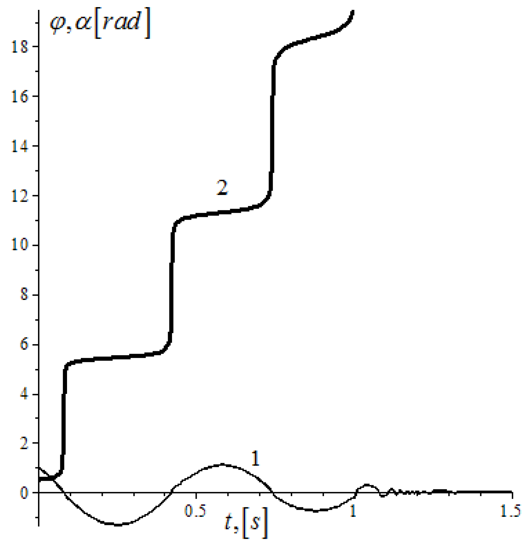
Taking into account Equation (20), the system of Equation (19) is solved remarkably. The dependences of α ( t ) and φ ( t ) at k 2 = γ = 0.1 and ε = 0.02 are illustrated by 
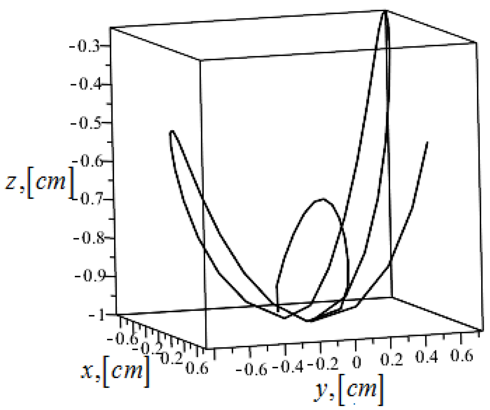
Figure 2. The three-dimensional trajectory of the ball in motion is found due to the numerical simulation of Equation (19) with the condition that the radius of the sphere is equal to the unity, and this is demonstrated in 
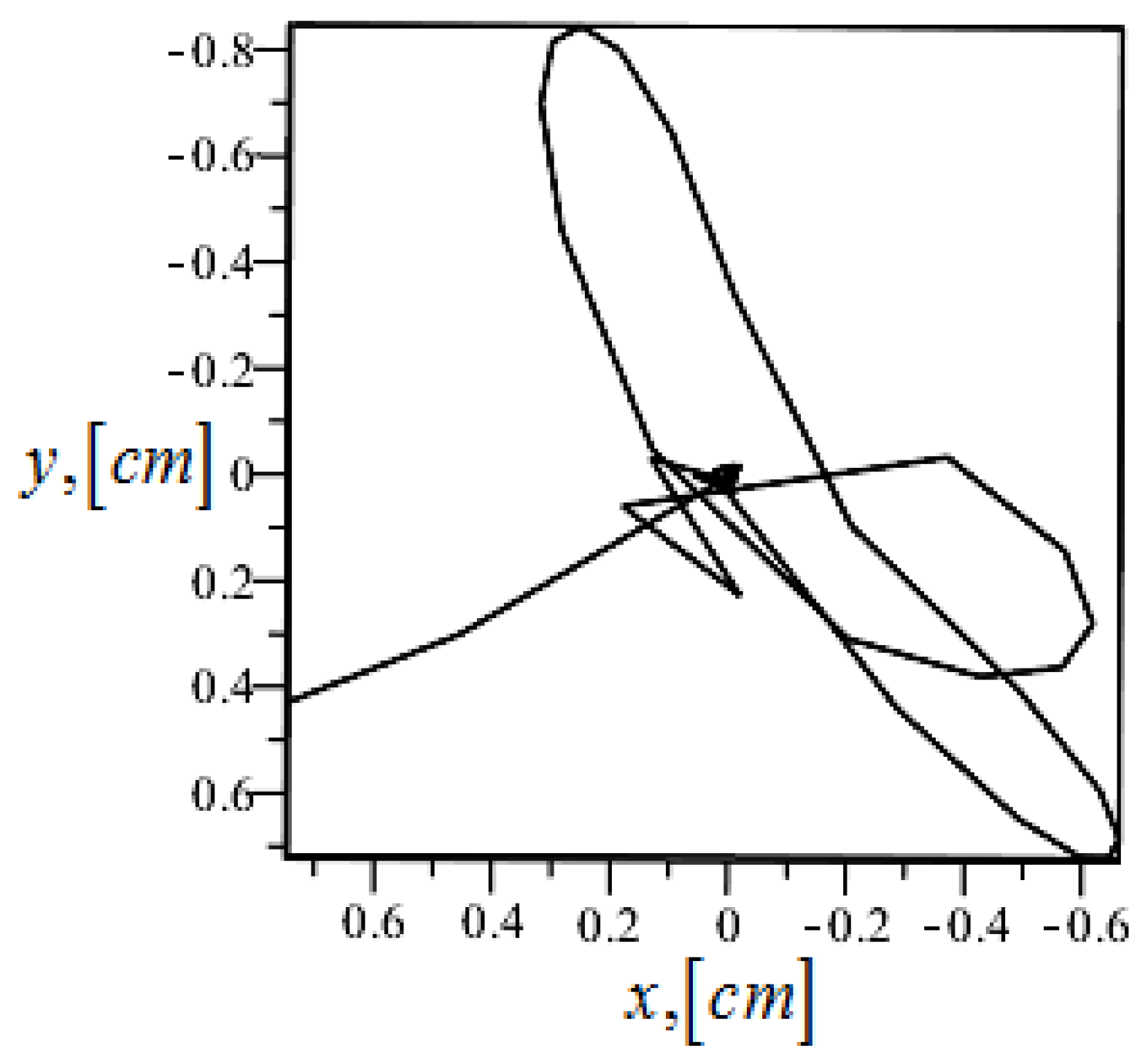
Figure 3. In accordance with these numerical solutions due to the transformations 3–5 of Equation (19), we can also find the trajectories of the motion in the projections on the coordinate planes x y ,   y z ,   x z . In Figure 4, as an example, is illustrated the corresponding dependence in the plane x y .
We should notice that due to the lower transformations of Equation (9), we can also calculate the dependence of the reaction force of the shell when the ball moves between spherical surfaces. In this case, for the interruption values of the angle parameter α , the reaction force will aperiodically “jump” in the condition that all changes of the parameters are continuous.
Moreover, we would like to pay attention to the case if we use the mathematical apparatus of the Euler angles α , β , γ (see, for example, the monograph [6]), where the description of the dynamics of the motion of the body between the surfaces of arbitrary shapes will be more complex. This problem will be addressed in a separate paper.

3. Conclusions

In the conclusion of this article, we would like to highlight some main results of the abovementioned research.
  • The fundamental system of the nonlinear differential equations is obtained, which describes the dynamics of the ball moving between two concentric spheres. In this system, taken into account is the dry friction of the ball on the surfaces, as is the dynamic viscosity of the fluid η filling the space between the spheres;
  • The analysis of the solution of the differential equations was carried out in both cases: in the ideal case and with the allowance of dissipative forces;
  • The time dependencies of the angular coordinates θ = π α and φ are calculated. Moreover, using the methods of numerical integration, it was illustrated a three-dimensional trajectory of the ball’s motion along the spherical surface, as well as its projection on the planes x y ,   y z ,   x z .

Author Contributions

S.G. and S.B. contributed equally to the writing of the main manuscript’s text and preparation of the figures. Both authors reviewed the manuscript. Both authors contributed equally to the paper.

Acknowledgments

We would like to express our appreciation for Professor Hovik Matevossian for his keen interest in this paper and his ambition to fulfill all the potential of our article.

Conflicts of Interest

The authors declare no conflict of interest.

References

  1. Appel, P. Theoretical Mechanics; Fizmatlit: Moscow, Russian, 1960. [Google Scholar]
  2. Shain, Y.F. An investigation of a system of equations describing the motion of a spherical pendulum in the case of the presence of resistance. Differ. Equ. 1967, 3, 1477–1483. [Google Scholar]
  3. Gladkov, S.О.; Bogdanova, S.B. Geometrical phase transition in the problem of the brachistochrone with friction. Mem. Fac. Phys. Lomonosov Mosc. State Univ. 2016, 1, 161001-1-5. Available online: http://uzmu.phys.msu.ru (accessed on 30 November 2018).
  4. Gladkov, S.О.; Bogdanova, S.B. To the theory of motion of a ball along a rotating brachistochrone with the account of the friction forces. Mem. Fac. Phys. Lomonosov Mosc. State Univ. 2017, 1, 171101-1-5. Available online: http://uzmu.phys.msu.ru (accessed on 30 November 2018).
  5. Landau, L.D.; Lifshitz, Е.М. Hydrodynamics; Fizmatlit: Moscow, Russian, 2001; ISBN 5-9221-0121-8. [Google Scholar]
  6. Landau, L.D.; Lifshitz, Е.М. Mechanics; Fizmatlit: Moscow, Russian, 2004; ISBN 5-9221-0055-6. [Google Scholar]
Figure 1. The geometry of the problem. In this figure, concentric circles are used for representation, but it is clear that in the stereometry, they are ellipses. For the simplification of the figure, they are shown as circles. R —a vector of mean radius; n = R R —a unit normal vector, where n = n 2 n 1 ; τ 1 —a unit tangential vector (see the main text of the paper); τ 2 —a unit tangential vector to the instantaneous circle of radius ρ , which is perpendicular to the axis z ; n a normal unit vector to this circle (it is lying in the plane of ( n τ 1 ) ; v —a momentary velocity, decomposed into a single instantaneous basis τ 1 and τ 2 ; m g —gravitational force; F c —resistant force directed against velocity vector v and tangential to the surface of the outer sphere. N —reaction force, θ —angle in azimuth, φ —polar bearing of the spherical coordinate system, angle α = π θ .
Mca 23 00077 g001
Figure 2. Line 1 shows the time law of the angle in azimuth α ( t ) ; Line 2 shows the time law of the polar bearing φ ( t ) . Initial conditions for this problem are α ( 0 ) = π 3 , φ ( 0 ) = π 6 , α ˙ ( 0 ) = 10 , φ ˙ ( 0 ) = 1 , if the parameters are k 2 = γ = 0.1 and ε = 0.02 .
Mca 23 00077 g002
Figure 3. Trajectory of the moving ball in three-dimensional dimensions for the initial conditions: α ( 0 ) = π 3 , φ ( 0 ) = π 6 , α ˙ ( 0 ) = 10 , φ ˙ ( 0 ) = 1 , if the parameters are k 2 = γ = 0.1 .
Mca 23 00077 g003
Figure 4. The projection of the three-dimensional trajectory of the ball, as illustrated in Figure 3, onto the plane x y .
Mca 23 00077 g004

