Abstract
Dynamical systems play a vital role in studying highly non-linear phenomena. One of the families of the dynamical systems is integer sequences. There is an integer sequence called Q-sequence: Q(n) = Q(n − Q(n − 1)) + Q(n − Q(n − 2)); for n = 3, 4, …; and Q(1) = Q(2) = 1. It exhibits a unique chaotic-order that might help develop approximate models of highly nonlinear phenomena. We explore this possibility and show how to modify a segment of the Q-sequence so that the modified segment becomes an approximate model of surface roughness (a highly non-linear phenomena that results from the material removal processes (e.g., turning, milling, grinding, and so on). The Q-sequence-based models of surface roughness can be used to recreate the surface heights whenever necessary. As such, it is a helpful means for developing simulation systems for virtual manufacturing.
1. Introduction
We often measure the dimensions, forms, and surfaces of artificial artifacts and see whether they are consistent with the given specifications. This has created a discipline of study called metrology. International standards have been developed to systematize the activities underlying this discipline [1]. A great deal of research has been conducted to develop reliable electro-mechanical devices for dimensional, form, and surface metrology [2,3,4,5]. Particularly in surface metrology [6], we deal with the heights of a machined surfaces measured by contact or non-contact instruments [4,5,6]. International standards provide a set of standards to measure the surface heights and then to process (filter [7], and quantify) them for surface characterization [1]. According to these standards, for example, the roughness of a machined surface is often quantified by such standard parameters as arithmetic average height Ra, peak-to-valley height Rz, fractal dimension, and so on [8]. Sometimes, non-conventional parameters, e.g., entropy [8], are also used for quantifying the surface roughness. Some authors have worked on the uncertainty modeling of surface roughness using probability-distribution-neutral representation, e.g., possibility distributions and fuzzy numbers [8]. Nowadays, we have Web-based systems, e.g., the system developed by the National Institute of Standards and Technology (NIST, Gaithersburg, MD, USA) [9], by which one can determine the standard roughness parameters online [1]. In addition, to share the evaluated surface roughness, efforts have been made to create web-based data, e.g., XML data incorporating the information of Ra [10]. Even though we characterized a surface by using Ra, Rz, entropy, fractal dimension, and possibility distribution, an individual/system who/that receives this information will not be able to recreate the surface heights. This means that we lose the surface height dynamics if we use the conventional quantification process described above. Thus, we need another means to capture the dynamics of surface roughness so that the individual/system) who/that) receives it can recreate it whenever necessary. It has been stressed that the manufacturing phenomena (e.g., the cutting force and even the surface roughness) are highly non-linear and can be modeled, in principle, by stationary and non-stationary Gaussian processes [11,12,13]. A surface roughness profile, in particular, consists of certain stochastic features [11], and to recreate the heights of a surface roughness profile, i.e., to capture the dynamics underlying a surface roughness profile, one needs to model these features using stochastic formulations [11,14]. This issue of dynamic representation of surface roughness has become even more important due to the advent of Internet of Things (IoT) [15], as schematically illustrated in Figure 1.
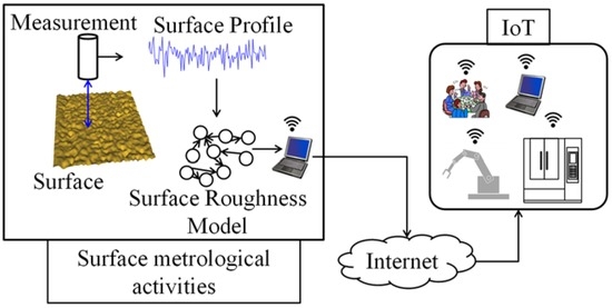
Figure 1.
Surface metrological activities from the viewpoint of Internet of Things (IoT).
IoT involved in the manufacturing systems requires cyber-physical systems [15,16,17,18] where the hardware and software systems will not only share the static data of non-linear phenomena of manufacturing activities but also the models that are capable of storing and sharing the underlying dynamics. A scenario of such futuristic systems is schematically shown in Figure 1 where the surface metrology activities are considered as an example. As seen from Figure 1, as far as the IoT is concerned, not only surface roughness quantification but also the modeling of surface heights is important for surface metrology. The model must capture the dynamics of the surface roughness so that it (the model) can recreate the surface heights whenever necessary in IoT-based systems, as schematically illustrated in Figure 1.
However, numerous authors have developed methods and tools to capture the dynamics of machined surface heights. For example, Wu [19] developed a methodology to simulate engineered surfaces using Fast Fourier Transform (FFT) where a given spectral density or auto-correlation function (ACF) is used as a means to model the irregular heights of a surface. Higuchi et al. [20] applied the concept of fractional Brownian motion (fBm) to simulate the surface heights of grinding wheels. Ullah et al. [21] developed a dynamical system that operates on some fuzzy if–then rules to simulate the surface roughness heights. Here, the fuzzy if–then rules are extracted from a given surface roughness profile. Ullah et al. [11] considered that the surface heights of a machined surface consist of four features, namely, trend, cycle, irregularities, and burst. They developed a stochastic model to organize these features and to recreate surface heights. Uchidate et al. [22] introduced an auto-regression based model to create surface heights for the sake of soft-calibration. Sharif Ullah et al. [23] modeled the microscopic interactions between workpiece and tool (e.g., a grinding wheel) that are stochastic in nature to simulate the surface heights of a machined surface for several passes. Nevertheless, the methodologies developed so far to capture the dynamics of surface roughness, e.g., the methodologies described in [11,19,20,21,22,23] and in the references therein, are parameter-dependent, requiring a great deal of efforts of the users to set the right values of a relatively large number of parameters. Therefore, a simpler but user-friendly methodology is needed to model the dynamics of the surface roughness. From this contemplation, this article is written. In particular, an integer sequence called the Q-sequence [24] will be employed to create a model of a surface profile. The remainder of this article is organized as follows:
Section 2 describes the main features of the Q-sequence. Section 3 describes a modification process of the Q-sequence. Section 4 describes how to create an approximate model of surface profile heights using a modified Q-sequence. Section 5 provides the discussions and concluding remarks of this article.
2. Q-Sequence
This section describes the main features of Q-sequence. Hofstadter introduced a dynamical system consisting of integers called Q-sequence [24] as follows:
In Equation (1), n is a natural number, i.e., n = 1, 2, 3, 4, etc. The first 100 values of Q(n) are as follows: 1, 1, 2, 3, 3, 4, 5, 5, 6, 6, 6, 8, 8, 8, 10, 9, 10, 11, 11, 12, 12, 12, 12, 16, 14, 14, 16, 16, 16, 16, 20, 17, 17, 20, 21, 19, 20, 22, 21, 22, 23, 23, 24, 24, 24, 24, 24, 32, 24, 25, 30, 28, 26, 30, 30, 28, 32, 30, 32, 32, 32, 32, 40, 33, 31, 38, 35, 33, 39, 40, 37, 38, 40, 39, 40, 39, 42, 40, 41, 43, 44, 43, 43, 46, 44, 45, 47, 47, 46, 48, 48, 48, 48, 48, 48, 64, 41, 52, 54, and 56. Figure 2 shows the nature of Q(n) ∈ ℵ+ for n ≤ 2000 (i.e., relatively small values of n). Pinn [25] studied the chaotic behavior that Q(n) exhibits for both small and large values of n. Some of the characteristics reported in [25] are as follows: (1) On short scales, Q(n) looks chaotic having groups of generations of sequences. (2) The k-th generation has 2k members which have “parents” mostly in the generation k − 1, and a few from the generation k − 2. In other words, in a short scale, a segment of Q(n) consists of integers that are close to each other. (3) Q(n) has bursts with increasing amplitude and length. (4) The trend in Q(n) disappears if the integer part of n/2 is subtracted. This is true if n is relatively small.
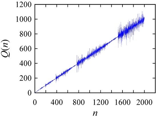
Figure 2.
The nature of the Q-sequence for small values of n.
This results in another integer sequence denoted as S(n) ∈ ℑ and given as
Figure 3 shows the time series plot of S(n) for the small values of n. As seen from Figure 3, similar to Q(n), S(n) also shows bursts at intervals n = 3, 6, 12, 24, 48, 96, etc. However, the trend seen in Q(n) disappears in the case of S(n). It can be modified in different ways to model non-linear signals. This issue is elaborated in the subsequent sections taking the case of surface roughness modeling.
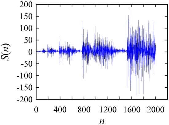
Figure 3.
The nature of S(n) for small values of n.
3. Modifying the Q-Sequence
This section shows a simple but useful modification technique of Q-sequence for the sake of modeling non-linear signals. Here, the Q-sequence refers to its trendless counterpart, i.e., S(n). In particular, a small segment of S(n) between two consecutive bursts can be used to create an approximate model of highly nonlinear signals, e.g., cutting force and surface roughness. The modification process uses successive linear interpolations that gradually expand a small segment of S(n). The formal description of this modification process is as follows.
Let S(n1,n2) be a segment of S(n), where n2 > n1, as follows:
Let us consider a segment of S(n), S(n1 = 1000, n2 = 1200). This segment is taken between two consecutive bursts of S(n). The time series plot and the return-map of this segment are shown in Figure 4.
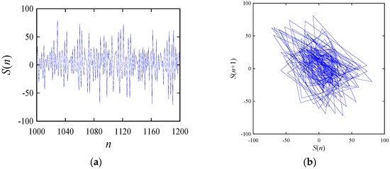
Figure 4.
The time series and return-map of S(1000,1200): (a) time series; (b) return-map.
In general, a return-map (or delay map) is a point-cloud that consists of a set of ordered-pairs or points of the nature {(y(t),y(t + j)) ∈ ℜ2 | t = 0,1, …, ∃j ∈ {1, 2, …}} created from a time series y(t) ∈ ℜ, t = 0, 1, etc. It can represent the hidden order underlying the parameter considered, which is difficult to grasp from the time series plot alone. For this reason, when one studies a non-linear behavior or dynamical system, e.g., S(n), return-maps are prepared along with the time series to attain more insights into it [26]. This role of the return-map can be understood clearly when one compares the time series plots and the return-maps shown in the remainder of this article.
However, one can modify S(n1,n2) by adding more integers without destroying its apparent look. The easiest way to achieve this is to add an integer at the middle of every two consecutive integers of S(n1,n2). To be more specific, let R(t,1) be an integer sequence wherein all integers of S(n1,n2) are included in addition to the integers that are the integer parts of the average of every two consecutive points of S(n1,n2). Therefore, the following formulation holds:
In Equation (4), a = n2 − n1 or n2 − n1 − 1, if it is an even or odd number, respectively.
Figure 5 shows the time series plot and the return map of R(t,1) corresponding to S(n1 = 1000, n2 = 1200). The difference between S(1000,1200) and R(t,1) is not visible from their time series plots as shown in Figure 4 and Figure 5, respectively, whereas their difference is visible when the return-maps as shown in Figure 4 and Figure 5 are compared. In particular, the return-map shown in Figure 4 is more scattered compared to that shown in Figure 5. This means that the gap between two consecutive points in Figure 5 is smaller than that in Figure 4, which is expected.
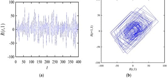
Figure 5.
The time series and return-map of R(t,1) corresponding to S(1000,1200): (a) time series; (b) return-map.
If needed, R(t,1) can be expanded further, as follows:
In Equation (5), ∀i ∈ {1, 2, …}. For example, Figure 6 and Figure 7 show the time series plots and return-maps of the integer sequences R(t,2) and R(t,3) found after applying the linear interpolation, as defined in Equation (5), to R(t,1) and R(t,2), respectively.
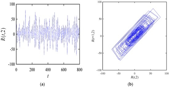
Figure 6.
The time series and return-map of R(t,2) corresponding to S(1000,1200): (a) time series; (b) return-map.
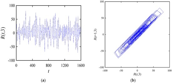
Figure 7.
The time series plot and return-map of R(t,3) corresponding to S(1000,1200): (a) time series; (b) return-map.
As a synopsis, the following remarks can be made: (a) All return maps of R(t,i), i = 1, 2, 3, follow a trend—a straight line with a unit slope. (b) The spread of the points in all return-maps decreases with the increase in the number of points in the sequence or decreases with the increase in i. (c) Most of the points in the return maps are located at the middle portion and relatively fewer points are located at two extremes. (d) The return-maps of two nearby R(t,i), i.e., R(t,1) and R(t,2) or R(t,2) and R(t,3), are somewhat similar but the return-maps of the sequences that are relatively far from each other in terms of i (here, R(t,1) and R(t,3)) look significantly different. Therefore, while modeling a highly irregular set of data points (e.g., the data points representing the heights of a processed surface), one must consult both the time series plot and its return-map. This strategy will be used to model a surface roughness profile, as described in the next section.
4. Modeling Surface Roughness
This section describes how to model a surface roughness profile using the integer sequences, R(t,i), i = 1, 2, …
First, consider a surface roughness profile denoted as z(t) ∈ ℜ, i = 0, 1, …, 250, and its return-map {(z(t),z(t + 1)) | i = 0, …, 250}, as shown in Figure 8. This surface roughness profile is one of the surface roughness profiles found while (surface) grinding a specimen made of glass using a Cubic Boron Nitride (cBN) grinding wheel in different grinding conditions. The experiments were performed at the Kitami Institute of Technology under the supervision of the author. A non-contact surface metrology instrument measures the primary profile of the ground surfaces. The NIST Surface Metrology Algorithm Testing System [27] removes the form error from the primary profile. No other filtering was applied to remove the waviness from the surface heights obtained after removing the form error. One can calculate the standard roughness parameters as prescribed in the ISO standard [1] using the surface heights shown in Figure 8. Calculating the values of these parameters does not preserve the dynamics of the roughness profile. Instead, if one can establish a model of the dynamics of the roughness profile, then it (the established model) can be used within the framework of IoT [14,15,16,17,18], or any other means, to recreate the profile heights. From the recreated profile heights, the standard roughness parameters can be calculated, if needed. This means that to achieve the cyber-physical system [14,15,16,17,18] of the surface metrology, it is more meaningful to create a model of the dynamic of the roughness profile than to just calculate the values of the roughness parameter. From this viewpoint, this section describes a procedure to modify the integer sequences, particularly, the ones given by R(t,i). The goal is to make it a model of the surface roughness heights or to store the dynamics of the surface roughness for the sake of recreation.
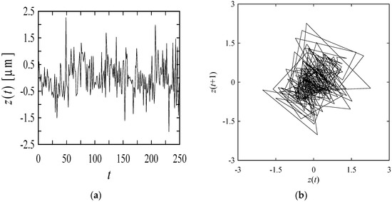
Figure 8.
A surface profile and its return-map: (a) surface heights; (b) return-map.
For the sake of modeling, the surface roughness profile shown in Figure 8 has been expanded by the linear interpolation using the procedure defined in Equations (4) and (5). (Note that the operation denoted as Int is not performed this time). The profile after the second linear interpolation denoted as z(t,2) is shown in Figure 9 in terms of the time series plot and return-map. The return-map shown in Figure 9 exhibits similar irregularities compared to that of R(t,3) (Figure 7). This means that R(t,3) has a potential to become a model of the interpolated roughness profile z(t,2).
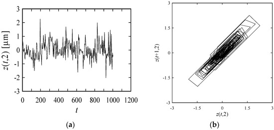
Figure 9.
The time series plot and return-map of the linear interpolated roughness profile: (a) time series; (b) return-map.
To make the comparison between R(t,3) and z(t,2) even more meaningful, R(t,3) can be scaled to z(t) and then shifted by an amount α ∈ ℜ (a small real number), resulting in a time series V(t) as follows:
In Equation (6), zmax = max(z(t) | t = 0, 1, …), zmin = min(z(t) | t = 0, 1, …), rmax = max(R(t,3) | t = 0, 1, …), and rmin = min(R(t,3) | t = 0, 1, …). If needed, one can add noises using a stochastic process, e.g., a noise that follows normal distribution [28], to V(t) to make it even more meaningful. The idea of adding such a stochastic noise is kept out of the scope of this article, however.
For the sake of visual inspection, the segments of V(t) and z(t,2) for t = 0, 1, …, 500, are shown in the same plot (Figure 10), where zmax = 2.260563913, zmin = −2.020452268, rmax = 81, rmin = −72, and α = −0.1. As seen from time series plots in Figure 10, both segments show a similar kind of variability. The similarity between the variability is more evident in the plot of the return-maps. In particular, both return-maps overlap and have almost the identical returns from one point to another.
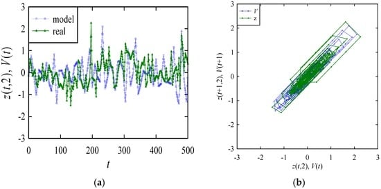
Figure 10.
Comparison between the model and real surface roughness profiles: (a) time series; (b) return-map.
How about the quantitative similarities between V(t) (the model) and z(t,2) (real surface roughness)? To answer this question, the values of Ra, Rz, and Entropy are calculated as described in [8]. The results are summarized in Table 1. As seen from Table 1, Rz is the same for both model and real surface roughness profiles, whereas Ra of the model surface roughness is greater than that of the real surface roughness profile, and Entropy of the model surface roughness is less than that of the real surface roughness profile. This difference in Entropy refers to the fact that the real surface roughness heights exhibit more complexity than those of the model.

Table 1.
Comparison between real and model surface roughness profiles.
To gain more insight into the quantitative similarities between V(t) and z(t,2), possibility distributions can be constructed using the respective point-clouds (return-maps), as shown in Figure 10. A possibility distribution (or a fuzzy number) is a probability-distribution-neutral representation of the irregularity associated with a variable [28]. It helps compare two roughness profiles, too, as shown in [8]. Thus, the possibility distributions of the return-maps of V(t) and z(t,2) have been constructed using the procedure described in [28]. The results are shown in Figure 11. It is worth mentioning that the possibility distribution produces a more reliable quantification of uncertainties associated with physical quantities, e.g., the works described in [29,30] where possibility distributions have been used to quantify the uncertainties associated with materials properties of some natural materials..
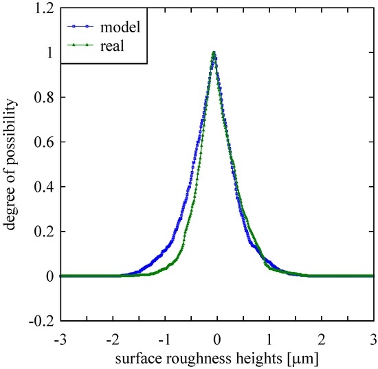
Figure 11.
Comparison between real surface roughness and its model in terms of the degree of possibility.
As seen from Figure 11, the shapes of the possibility distributions are identical except for surface roughness heights in the range [−1.5, −0.5] μm, i.e., in the range located on the left hand side of the pick. For both cases, on the other hand, the picks are at about 0 μm.
The above descriptions collectively refer to the fact that a signal V(t) derived from Q-sequence approximately models the dynamics of a surface roughness profile.
5. Discussion and Concluding Remarks
The results reported in Section 2, Section 3 and Section 4 collectively refer to a procedure of modeling the heights of a surface profile, as schematically illustrated in Figure 12. As seen from Figure 12, the following steps can be exhausted for modeling.
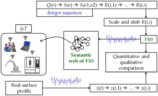
Figure 12.
Schematic diagram of dynamic modeling of surface profile using Q-sequence.
- Step 1
- Generate Q(n) (Equation (1)).
- Step 2
- Generate S(n) (Equation (2)).
- Step 3
- Select a segment of S(n), S(n1,n2) (Equation (3)).
- Step 4
- Expand S(n1,n2) by a linear interpolation operation and generate R(t,1) (Equation (4)).
- Step 5
- Expand R(t,1) by successive linear interpolation and generate R(t,i), i = 1, 2, … (Equation (5)).
- Step 6
- Select one of the R(t,i), ∃i ∈{1, 2, …}.
- Step 7
- Scale and shift R(t,i) selected in Step 6 and generate V(t) (Equation (6)).
- Step 8
- Compare V(t) with the given surface profile z(t) or with one of its (z(t)’s) linear interpolated profiles, z(t,j), j = 1, 2, etc.
- Step 9
- If the comparison is satisfactory in terms of qualitative and quantitative measures, then accept V(t) as a model of the roughness profile. Create semantic web to use V(t) in the framework of IoT. Otherwise, go back to Step 3 and continue.
Although the above procedure is applied to surface roughness only, it can also be applied to model other nonlinear signals such as cutting force. This issue can be explored further. Nevertheless, when one has the models that mimic the dynamics of various non-linear phenomena of the manufacturing process, it would not be difficult to build the cyber-physical systems for the seamless transfer of knowledge and information of the manufacturing processes from one system to another within the framework of IoT. This means that the methodologies like the one described here will become the valuable constituents of the manufacturing systems in the years to come, i.e., in the era of Industry 4.0. This also means that the devices developed for forms and surface metrology, e.g., the ones described in [2,3,4,5], require systems aided by the methodology described here to make them compatible with Industry 4.0.
Acknowledgments
An initial short version of the work presented here has been published in the Proceedings of the Ninth CIRP Workshop on Modeling of Machining Operations, 11–12 May 2006, Bled, Slovenia (pp. 431–437).
Conflicts of Interest
The author declares no conflicts of interest.
References
- ISO TC 213. Available online: http://www.iso.org/iso/home/store/catalogue_tc/catalogue_tc_browse.htm?commid=54924&published=on (accessed on 15 January 2017).
- Jusko, O.; Neugebauer, M.; Reimann, H.; Bernhardt, R. Recent progress in CMM-based form measurement. Int. J. Autom. Technol. 2015, 9, 170–175. [Google Scholar]
- Woźniak, A.; Krajewski, G. CMM dynamic properties of the scanning measurement of a 2D profile. Int. J. Autom. Technol. 2015, 9, 530–533. [Google Scholar]
- Ito, S.; Jia, Z.; Goto, S.; Hosobuchi, K.; Shimizu, Y.; He, G.; Gao, W. An electrostatic force probe for surface profile measurement in noncontact condition. Int. J. Autom. Technol. 2013, 7, 714–719. [Google Scholar]
- Elrawemi, M.; Blunt, L.; Muhamedsalih, H.; Gao, F.; Fleming, L. Implementation of in Process Surface Metrology for R2R flexible PV barrier films. Int. J. Autom. Technol. 2015, 9, 312–321. [Google Scholar]
- Whitehouse, D. A new look at surface metrology. Wear 2009, 266, 560–565. [Google Scholar] [CrossRef]
- Wang, X.; Shi, T.; Liao, G.; Zhang, Y.; Hong, Y.; Chen, K. Using Wavelet Packet Transform for Surface Roughness Evaluation and Texture Extraction. Sensors 2017, 17, 933. [Google Scholar] [CrossRef] [PubMed]
- Sharif Ullah, A.M.M.; Fuji, A.; Kubo, A.; Tamaki, J.; Kimura, M. On the surface metrology of bimetallic components. Mach. Sci. Technol. 2015, 19, 339–359. [Google Scholar] [CrossRef]
- Bui, S.H.; Vorburger, T.V. Surface metrology algorithm testing system. Precis. Eng. 2007, 31, 218–225. [Google Scholar] [CrossRef]
- Li, T.; Blunt, L.A.; Jiang, X.; Zeng, W. An Information Model for Surface Metrology. Procedia CIRP 2013, 10, 251–258. [Google Scholar] [CrossRef]
- Sharif Ullah, A.M.M.; Tamaki, J.; Kubo, A. Modeling and Simulation of 3D Surface Finish of Grinding. Adv. Mater. Res. 2010, 126–128, 672–677. [Google Scholar] [CrossRef]
- Sharif Ullah, A.M.M.; Harib, K.H. Simulation of Cutting Force using Nonstationary Gaussian Process. J. Intell. Manuf. 2010, 21, 681–691. [Google Scholar] [CrossRef]
- Pawlus, P. Simulation of Stratified Surface Topographies. Wear 2008, 264, 457–463. [Google Scholar] [CrossRef]
- Sharif Ullah, A.M.M.; Arai, N.; Watanabe, M. Concept Map and Internet-aided Manufacturing. Procedia CIRP 2013, 12, 378–383. [Google Scholar] [CrossRef]
- Weyer, S.; Schmitt, M.; Ohmer, M.; Gorecky, D. Towards Industry 4.0—Standardization as the crucial challenge for highly modular, multi-vendor production systems. IFAC-PapersOnLine 2015, 48, 579–584. [Google Scholar] [CrossRef]
- Monostori, L. Cyber-physical Production Systems: Roots, Expectations and R&D challenges. Procedia CIRP 2014, 17, 9–13. [Google Scholar]
- Ramos, L. Semantic Web for manufacturing, trends and open issues: Toward a state of the art. Comput. Ind. Eng. 2015, 90, 444–460. [Google Scholar] [CrossRef]
- Lee, J.; Bagheri, B.; Kao, H.-A. A Cyber-Physical Systems architecture for Industry 4.0-based manufacturing systems. Manuf. Lett. 2015, 3, 18–23. [Google Scholar] [CrossRef]
- Wu, J.-J. Simulation of rough surfaces with FFT. Tribol. Int. 2000, 33, 47–58. [Google Scholar] [CrossRef]
- Higuchi, M.; Yamaguchi, T.; Yano, A.; Yamamoto, N.; Ueshima, R.; Matumori, N.; Yoshizawa, I. Development of Design Technology of Porous Superfinishing Stone Using Fractal Geometry (2nd Report)—Geometric Modeling of Stone Topography and Design Support System. J. Jpn. Soc. Precis. Eng. 2001, 67, 428–432. (In Japanese) [Google Scholar] [CrossRef]
- Ullah, A.M.M.S.; Harib, K.H. Knowledge extraction from time series and its application to surface roughness simulation. Inf. Knowl. Syst. Manag. 2006, 5, 117–134. [Google Scholar]
- Uchidate, M.; Yanagi, K.; Yoshida, I.; Shimizu, T.; Iwabuchi, A. Generation of 3D random topography datasets with periodic boundaries for surface metrology algorithms and measurement standards. Wear 2011, 271, 565–570. [Google Scholar] [CrossRef]
- Sharif Ullah, A.M.M.; Chowdhury, M.A.K.; Kubo, A. A Surface Generation Mechanism of Grinding. Appl. Mech. Mater. 2017, 860, 13–18. [Google Scholar] [CrossRef]
- Hofstadter, D.R. Gödel, Escher, Bach: An Eternal Golden Braid; Vintage Books: New York, NY, USA, 1980; pp. 137–138. [Google Scholar]
- Pinn, K. Order and chaos in Hofstadter’s Q(n) sequence. Complexity 1999, 4, 41–46. [Google Scholar] [CrossRef]
- Kantz, H.; Schreiber, T. Nonlinear Time Series Analysis; Cambridge University Press: Cambridge, UK, 2002. [Google Scholar]
- NIST Surface Roughness Database. Available online: http://physics.nist.gov/VSC/jsp/Database.jsp (accessed on 12 January 2017).
- Sharif Ullah, A.M.M.; Shamsuzzaman, M. Fuzzy Monte Carlo Simulation using point-cloud-based probability-possibility transformation. Simulation 2013, 89, 860–875. [Google Scholar] [CrossRef]
- Ullah, A.M.M.S.; Shahinur, S.; Haniu, H. On the Mechanical Properties and Uncertainties of Jute Yarns. Materials 2017, 10, 450. [Google Scholar] [CrossRef]
- Shahinur, S.; Ullah, A.M.M.S. Quantifying the Uncertainty Associated with the Material Properties of a Natural Fiber. Procedia CIRP 2017, 61, 541–546. [Google Scholar] [CrossRef]
© 2017 by the author. Licensee MDPI, Basel, Switzerland. This article is an open access article distributed under the terms and conditions of the Creative Commons Attribution (CC BY) license (http://creativecommons.org/licenses/by/4.0/).