A New Smoothing Nonlinear Penalty Function for Constrained Optimization

Abstract

In this study, a new smoothing nonlinear penalty function for constrained optimization problems is presented. It is proved that the optimal solution of the smoothed penalty problem is an approximate optimal solution of the original problem. Based on the smoothed penalty function, we develop an algorithm for finding an optimal solution of the optimization problems with inequality constraints. We further discuss the convergence of this algorithm and test this algorithm with three numerical examples. The numerical examples show that the proposed algorithm is feasible and effective for solving some nonlinear constrained optimization problems.

1. Introduction

Consider the following constrained optimization problem:

$$\begin{array}{cc}\hfill (P)min& f(x)\hfill \\ \hfill \mathrm{s}.\mathrm{t}.& g_i(x)\le 0,i=1,2,\dots ,m,\hfill \\ & x\in {\mathbb{R}}^n,\hfill \end{array}$$

where the functions $f,g_i:{\mathbb{R}}^n\to \mathbb{R},i\in I=\{1,2,\dots ,m\}$, are continuously differentiable functions.

Let $X_0=\{x\in {\mathbb{R}}^n|g_i(x)\le 0,i\in I\}$ be the feasible solution set and we assume that $X_0$ is not empty.

For a general constrained optimization problem, the penalty function method has attracted many researchers in both theoretical and practical aspects. However, to obtain an optimal solution for the original problem, the conventional quadratic penalty function method usually requires that the penalty parameter tends to infinity, which is undesirable in practical computation. In order to overcome the drawbacks of the quadratic penalty function method, exact penalty functions were proposed to solve problem $(P)$. Zangwill [1] first proposed the $l_1$ exact penalty function

$$F^1(x,\rho )=f(x)+\rho \sum _{i=1}^m{g}_i^{+}(x),$$

(1)

where $\rho >0$ is a penalty parameter, and $g_i^{+}(x)=max\{0,g_i(x)\},i=1,2,\dots ,m$. It was proved that there exists a fixed constant ${\rho }_0>0$, for any $\rho >{\rho }_0$, and any global solution of the exact penalty problem is also a global solution of the original problem. Therefore, the exact penalty function methods have been widely used for solving constrained optimization problems (see, e.g., [2,3,4,5,6,7,8,9]).

Recently, the nonlinear penalty function of the following form has been investigated in [10,11,12,13]:

$$F^k(x,\rho )={\left[f{(x)}^k+\rho \sum _{i=1}^m{(g_i^{+}(x))}^k\right]}^{\frac{1}{k}},$$

(2)

where $f(x)$ is assumed to be positive and $k\in (0,+\infty )$. It is called the k-th power penalty function in [14,15]. Obviously, if $k=1$, the nonlinear penalty function $F^k(x,\rho )$ is reduced to the $l_1$ exact penalty function. In [12], it was shown that the exact penalty parameter corresponding to $k\in (0,1]$ is substantially smaller than that of the $l_1$ exact penalty function. Rubinov and Yang [13] also studied a penalty function as follows:

$${\psi }_{\rho }^k(x,c)={[f(x)-c]}^k+\rho \sum _{i=1}^m{g}_i^{+}(x),$$

(3)

where $c\in \mathbb{R}$ such that $f(x)-c>0$ for any $x\in {\mathbb{R}}^n$, and $k\in (0,+\infty )$. The corresponding penalty problem of $(P)$ is defined as

$$\begin{array}{c}\hfill (P_{\rho })min{\psi }_{\rho }^k(x,c)\mathrm{s}.\mathrm{t}.x\in {\mathbb{R}}^n.\end{array}$$

In fact, the original problem $(P)$ is equivalent to the problem as follows:

$$\begin{array}{cc}\hfill (P^{\prime })min& {[f(x)-c]}^k\hfill \\ \hfill \mathrm{s}.\mathrm{t}.& g_i(x)\le 0,i=1,2,\dots ,m,\hfill \\ & x\in {\mathbb{R}}^n.\hfill \end{array}$$

Obviously, the penalty problem $(P_{\rho })$ is the $l_1$ exact penalty problem of problem $(P^{\prime })$ defined as (1).

It is noted that these penalty functions $F^1(x,\rho ),F^k(x,\rho )(0<k\le 1)$ and ${\psi }_{\rho }^k(x,c)$ are not differentiable at x such that $g_i(x)=0$ for some $i\in I$, which prevents the use of gradient-based methods and causes some numerical instability problems in its implementation, when the value of the penalty parameter becomes large [3,5,6,8]. In order to use existing gradient-based algorithms, such as a Newton method, it is necessary to smooth the exact penalty function. Thus, the smoothing of the exact penalty function attracts much attention [16,17,18,19,20,21,22,23,24]. Pinar and Zenios [21] and Wu et al. [22] discussed a quadratic smoothing approximation to nondifferentiable exact penalty functions for constrained optimization. Binh [17] and Xu et al. [23] proposed a second-order differentiability technique to the $l_1$ exact penalty function. It is shown that the optimal solution of the smoothed penalty problem is an approximate optimal solution of the original optimization problem. Zenios et al. [24] discussed an algorithm for the solution of large-scale optimization problems.

In this study, we aim to develop the smoothing technique for the nonlinear penalty function (3). First, we define the following smoothing function $q_{ϵ,\rho }^k(t)$ by

$$\begin{array}{c}\hfill q_{ϵ,\rho }^k(t)=\left\{\begin{array}{cc}{\displaystyle 0}\hfill & \mathrm{if}t\le 0,\hfill \\ {\displaystyle \frac{2m^2{\rho }^2}{9{ϵ}^2}{t}^{3k}}\hfill & \mathrm{if}0\le t\le {\left(\frac{ϵ}{m\rho }\right)}^{\frac{1}{k}},\hfill \\ {\displaystyle t^k+\frac{ϵ}{3m\rho }{e}^{-\frac{m\rho }{ϵ}{t}^k+1}-\frac{10ϵ}{9m\rho }}\hfill & \mathrm{if}t\ge {\left(\frac{ϵ}{m\rho }\right)}^{\frac{1}{k}},\hfill \end{array}\right.\end{array}$$

where $0<k<+\infty ,\rho >0$ and $ϵ>0$. By considering this smoothing function, a new smoothing nonlinear penalty function is obtained. We use this smoothing nonlinear penalty function that is able to convert a constrained optimization problem into minimizations of a sequence of continuously differentiable functions and propose a corresponding algorithm for solving constrained optimization problems.

The rest of this paper is organized as follows. In Section 2, we propose a new smoothing penalty function for inequality constrained optimization problems, and some fundamental properties of its are proved. In Section 3, an algorithm based on the smoothed penalty function is presented and its global convergence is proved. In Section 4, we report results on application of this algorithm to three test problems and compare the results obtained with other similar algorithms. Finally, conclusions are discussed in Section 5.

2. Smoothing Nonlinear Penalty Functions

In this section, we first construct a new smoothing function. Then, we introduce our smoothing nonlinear penalty function and discuss its properties.

Let $q^k(t):\mathbb{R}\to \mathbb{R}$ be as follows:

$$\begin{array}{c}\hfill q^k(t)=\left\{\begin{array}{cc}{\displaystyle 0}\hfill & \mathrm{if}t\le 0,\hfill \\ {\displaystyle t^k}\hfill & \mathrm{if}t\ge 0,\hfill \end{array}\right.\end{array}$$

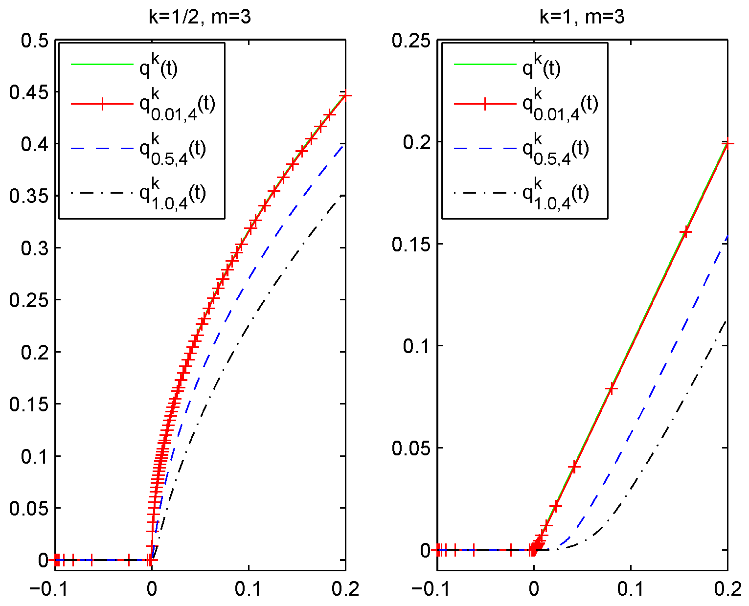
where $0<k<+\infty$. Obviously, the function $q^k(t)$ is $C^1$ on $\mathbb{R}$ for $k>1$, but it is not $C^1$ for $0<k\le 1$. It is useful in defining exact penalty functions for constrained optimization problems (see, e.g., [14,15,21]). Consider the nonlinear penalty function

$$F_{\rho }^k(x,c)={[f(x)-c]}^k+\rho \sum _{i=1}^m{q}^k(g_i(x)),$$

(4)

and the corresponding penalty problem

$$\begin{array}{c}\hfill (N{P}_{\rho })min{F}_{\rho }^k(x,c)\mathrm{s}.\mathrm{t}.x\in {\mathbb{R}}^n.\end{array}$$

As previously mentioned, for any $ϵ>0$ and $\rho >0$, the function $q_{ϵ,\rho }^k(t)$ is defined as:

$$\begin{array}{c}\hfill q_{ϵ,\rho }^k(t)=\left\{\begin{array}{cc}{\displaystyle 0}\hfill & \mathrm{if}t\le 0,\hfill \\ {\displaystyle \frac{2m^2{\rho }^2}{9{ϵ}^2}{t}^{3k}}\hfill & \mathrm{if}0\le t\le {\left(\frac{ϵ}{m\rho }\right)}^{\frac{1}{k}},\hfill \\ {\displaystyle t^k+\frac{ϵ}{3m\rho }{e}^{-\frac{m\rho }{ϵ}{t}^k+1}-\frac{10ϵ}{9m\rho }}\hfill & \mathrm{if}t\ge {\left(\frac{ϵ}{m\rho }\right)}^{\frac{1}{k}},\hfill \end{array}\right.\end{array}$$

where $0<k<+\infty$.

Figure 1 shows the behavior of $q^k(t)$ and $q_{ϵ,\rho }^k(t)$.

Figure 1. The behavior of $q^k(t)$ and $q_{ϵ,\rho }^k(t).$

In the following, we discuss the properties of $q_{ϵ,\rho }^k(t)$.

Lemma 1.

For $0<k<+\infty$ and any $ϵ>0$, we have

(i) 

$q_{ϵ,\rho }^k(t)$ is continuously differentiable for $k>\frac{1}{3}$ on $\mathbb{R}$, where

$${\left[q_{ϵ,\rho }^k(t)\right]}^{\prime }=\left\{\begin{array}{cc}{\displaystyle 0}\hfill & ift\le 0,\hfill \\ {\displaystyle \frac{2k{m}^2{\rho }^2}{3{ϵ}^2}{t}^{3k-1}}\hfill & if0\le t\le {\left(\frac{ϵ}{m\rho }\right)}^{\frac{1}{k}},\hfill \\ {\displaystyle k{t}^{k-1}-\frac{1}{3}k{t}^{k-1}{e}^{-\frac{m\rho }{ϵ}{t}^k+1}}\hfill & ift\ge {\left(\frac{ϵ}{m\rho }\right)}^{\frac{1}{k}}.\hfill \end{array}\right.$$

(ii) 

$\underset{ϵ\to 0}{lim}{q}_{ϵ,\rho }^k(t)=q^k(t)$.

(iii) 

$q^k(t)\ge q_{ϵ,\rho }^k(t),\forall t\in \mathbb{R}$.

Proof. 

(i) First, we prove that $q_{ϵ,\rho }^k(t)$ is continuous. Obviously, the function $q_{ϵ,\rho }^k(t)$ is continuous at any $t\in \mathbb{R}\backslash \left\{0,{(\frac{ϵ}{m\rho })}^{\frac{1}{k}}\right\}$. We only need to prove that $q_{ϵ,\rho }^k(t)$ continuous at the separating points: 0 and ${(\frac{ϵ}{m\rho })}^{\frac{1}{k}}$.

(1) For $t=0$, we have

$$\underset{t\to 0^{-}}{lim}{q}_{ϵ,\rho }^k(t)=\underset{t\to 0^{-}}{lim}0=0,\underset{t\to 0^{+}}{lim}{q}_{ϵ,\rho }^k(t)=\underset{t\to 0^{+}}{lim}\frac{2m^2{\rho }^2}{9{ϵ}^2}{t}^{3k}=0,$$

which implies

$$\underset{t\to 0^{-}}{lim}{q}_{ϵ,\rho }^k(t)=\underset{t\to 0^{+}}{lim}{q}_{ϵ,\rho }^k(t)=0=q_{ϵ,\rho }^k(0).$$

Thus, $q_{ϵ,\rho }^k(t)$ is continuous at $t=0$.

(2) For $t={(\frac{ϵ}{m\rho })}^{\frac{1}{k}}$, we have

$$\begin{array}{cc}\hfill \underset{t\to {\left[{(\frac{ϵ}{m\rho })}^{\frac{1}{k}}\right]}^{-}}{lim}{q}_{ϵ,\rho }^k(t)& =\underset{t\to {\left[{(\frac{ϵ}{m\rho })}^{\frac{1}{k}}\right]}^{-}}{lim}\frac{2m^2{\rho }^2}{9{ϵ}^2}{t}^{3k}=\frac{2ϵ}{9m\rho },\hfill \\ \hfill \underset{t\to {\left[{(\frac{ϵ}{m\rho })}^{\frac{1}{k}}\right]}^{+}}{lim}{q}_{ϵ,\rho }^k(t)& =\underset{t\to {\left[{(\frac{ϵ}{m\rho })}^{\frac{1}{k}}\right]}^{+}}{lim}\left[t^k+\frac{ϵ}{3m\rho }{e}^{-\frac{m\rho }{ϵ}{t}^k+1}-\frac{10ϵ}{9m\rho }\right]=\frac{2ϵ}{9m\rho },\hfill \end{array}$$

which implies

$$\underset{t\to {\left[{(\frac{ϵ}{m\rho })}^{\frac{1}{k}}\right]}^{-}}{lim}{q}_{ϵ,\rho }^k(t)=\underset{t\to {\left[{(\frac{ϵ}{m\rho })}^{\frac{1}{k}}\right]}^{+}}{lim}{q}_{ϵ,\rho }^k(t)=\frac{2ϵ}{9m\rho }=q_{ϵ,\rho }^k\left({(\frac{ϵ}{m\rho })}^{\frac{1}{k}}\right).$$

Thus, $q_{ϵ,\rho }^k(t)$ is continuous at $t={(\frac{ϵ}{m\rho })}^{\frac{1}{k}}$.

Next, we will show that $q_{ϵ,\rho }^k(t)$ is continuously differentiable, i.e., ${\left[q_{ϵ,\rho }^k(t)\right]}^{\prime }$ is continuous. Actually, we only need to prove that ${\left[q_{ϵ,\rho }^k(t)\right]}^{\prime }$ is continuous at the separating points: 0 and ${(\frac{ϵ}{m\rho })}^{\frac{1}{k}}$.

(1) For $t=0$, we have

$$\underset{t\to 0^{-}}{lim}{\left[q_{ϵ,\rho }^k(t)\right]}^{\prime }=\underset{t\to 0^{-}}{lim}0=0,\underset{t\to 0^{+}}{lim}{\left[q_{ϵ,\rho }^k(t)\right]}^{\prime }=\underset{t\to 0^{+}}{lim}\frac{2k{m}^2{\rho }^2}{3{ϵ}^2}{t}^{3k-1}=0,$$

which implies

$$\underset{t\to 0^{-}}{lim}{\left[q_{ϵ,\rho }^k(t)\right]}^{\prime }=\underset{t\to 0^{+}}{lim}{\left[q_{ϵ,\rho }^k(t)\right]}^{\prime }=0={\left[q_{ϵ,\rho }^k(0)\right]}^{\prime }.$$

Thus, ${\left[q_{ϵ,\rho }^k(t)\right]}^{\prime }$ is continuous at $t=0$.

(2) For $t={(\frac{ϵ}{m\rho })}^{\frac{1}{k}}$, we have

$$\begin{array}{cc}\hfill \underset{t\to {\left[{(\frac{ϵ}{m\rho })}^{\frac{1}{k}}\right]}^{-}}{lim}{\left[q_{ϵ,\rho }^k(t)\right]}^{\prime }& =\underset{t\to {\left[{(\frac{ϵ}{m\rho })}^{\frac{1}{k}}\right]}^{-}}{lim}\frac{2k{m}^2{\rho }^2}{3{ϵ}^2}{t}^{3k-1}=\frac{2k}{3}{\left(\frac{ϵ}{m\rho }\right)}^{\frac{k-1}{k}},\hfill \\ \hfill \underset{t\to {\left[{(\frac{ϵ}{m\rho })}^{\frac{1}{k}}\right]}^{+}}{lim}{\left[q_{ϵ,\rho }^k(t)\right]}^{\prime }& =\underset{t\to {\left[{(\frac{ϵ}{m\rho })}^{\frac{1}{k}}\right]}^{+}}{lim}\left(k{t}^{k-1}-\frac{1}{3}k{t}^{k-1}{e}^{-\frac{m\rho }{ϵ}{t}^k+1}\right)=\frac{2k}{3}{\left(\frac{ϵ}{m\rho }\right)}^{\frac{k-1}{k}},\hfill \end{array}$$

which implies

$$\underset{t\to {\left[{(\frac{ϵ}{m\rho })}^{\frac{1}{k}}\right]}^{-}}{lim}{\left[q_{ϵ,\rho }^k(t)\right]}^{\prime }=\underset{t\to {\left[{(\frac{ϵ}{m\rho })}^{\frac{1}{k}}\right]}^{+}}{lim}{\left[q_{ϵ,\rho }^k(t)\right]}^{\prime }=\frac{2k}{3}{\left(\frac{ϵ}{m\rho }\right)}^{\frac{k-1}{k}}={\left[q_{ϵ,\rho }^k\left({(\frac{ϵ}{m\rho })}^{\frac{1}{k}}\right)\right]}^{\prime }.$$

Thus, ${\left[q_{ϵ,\rho }^k(t)\right]}^{\prime }$ is continuous at $t={(\frac{ϵ}{m\rho })}^{\frac{1}{k}}$.

(ii) For $\forall t\in \mathbb{R}$, by the definition of $q^k(t)$ and $q_{ϵ,\rho }^k(t),$ we have

$$q^k(t)-q_{ϵ,\rho }^k(t)=\left\{\begin{array}{cc}{\displaystyle 0}\hfill & \mathrm{if}t\le 0,\hfill \\ {\displaystyle t^k-\frac{2m^2{\rho }^2}{9{ϵ}^2}{t}^{3k}}\hfill & \mathrm{if}0\le t\le {\left(\frac{ϵ}{m\rho }\right)}^{\frac{1}{k}},\hfill \\ {\displaystyle \frac{10ϵ}{9m\rho }-\frac{ϵ}{3m\rho }{e}^{-\frac{m\rho }{ϵ}{t}^k+1}}\hfill & \mathrm{if}t\ge {\left(\frac{ϵ}{m\rho }\right)}^{\frac{1}{k}}.\hfill \end{array}\right.$$

When $0\le t\le {\left(\frac{ϵ}{m\rho }\right)}^{\frac{1}{k}}$, let $u=t^k$. Then, we have $0\le u\le \frac{ϵ}{m\rho }$. Consider the function:

$$G(u)=u-\frac{2m^2{\rho }^2}{9{ϵ}^2}{u}^3,0\le u\le \frac{ϵ}{m\rho },$$

and we have

$$G^{\prime }(u)=1-\frac{2m^2{\rho }^2}{3{ϵ}^2}{u}^2,0\le u\le \frac{ϵ}{m\rho }.$$

Obviously, $G^{\prime }(u)>0$ for $0\le u\le \frac{ϵ}{m\rho }$. Moreover, $G(0)=0$ and $G(\frac{ϵ}{m\rho })=\frac{7ϵ}{9m\rho }$. Hence, we have

$$0\le q^k(t)-q_{ϵ,\rho }^k(t)\le \frac{7ϵ}{9m\rho }.$$

When $t\ge {\left(\frac{ϵ}{m\rho }\right)}^{\frac{1}{k}}$, we have

$$\begin{array}{c}\hfill 0<q^k(t)-q_{ϵ,\rho }^k(t)=\frac{10ϵ}{9m\rho }-\frac{ϵ}{3m\rho }{e}^{-\frac{m\rho }{ϵ}{t}^k+1}\le \frac{10ϵ}{9m\rho }.\end{array}$$

Thus, we have

$$0\le q^k(t)-q_{ϵ,\rho }^k(t)\le \frac{10ϵ}{9m\rho }.$$

That is,

$$\underset{ϵ\to 0}{lim}{q}_{ϵ,\rho }^k(t)=q^k(t).$$

(iii) For $\forall t\in \mathbb{R}$, from (ii), we have

$$\begin{array}{c}\hfill q^k(t)-q_{ϵ,\rho }^k(t)\ge 0,\end{array}$$

which is $q^k(t)\ge q_{ϵ,\rho }^k(t)$.

This completes the proof. ☐

In this study, we always assume that $c<0$ and $|c|$ is large enough, such that $f(x)-c>0$ for all $x\in {\mathbb{R}}^n$. Let

$$F_{ϵ,\rho }^k(x,c)={[f(x)-c]}^k+\rho \sum _{i=1}^m{q}_{ϵ,\rho }^k\left(g_i(x)\right),0<k<+\infty .$$

(5)

Then, $F_{ϵ,\rho }^k(x,c)$ is continuously differentiable at any $x\in {\mathbb{R}}^n$ and is a smooth approximation of $F_{\rho }^k(x,c)$. We have the following smoothed penalty problem:

$$\begin{array}{c}\hfill (N{P}_{ϵ,\rho })min{F}_{ϵ,\rho }^k(x,c)\mathrm{s}.\mathrm{t}.x\in {\mathbb{R}}^n.\end{array}$$

Lemma 2.

We have that

$$0\le F_{\rho }^k(x,c)-F_{ϵ,\rho }^k(x,c)\le \frac{10ϵ}{9},0<k<+\infty$$

(6)

for any $x\in {\mathbb{R}}^n,ϵ>0$ and $\rho >0$.

Proof. 

For any $x\in {\mathbb{R}}^n,ϵ>0,\rho >0$, we have

$$F_{\rho }^k(x,c)-F_{ϵ,\rho }^k(x,c)=\rho \sum _{i=1}^m\left(q^k(g_i(x))-q_{ϵ,\rho }^k(g_i(x))\right).$$

Note that

$$q^k(g_i(x))-q_{ϵ,\rho }^k(g_i(x))=\left\{\begin{array}{cc}{\displaystyle 0}\hfill & \mathrm{if}{g}_i(x)\le 0,\hfill \\ {\displaystyle {\left[g_i(x)\right]}^k-\frac{2m^2{\rho }^2}{9{ϵ}^2}{\left[g_i(x)\right]}^{3k}}\hfill & \mathrm{if}0\le g_i(x)\le {\left(\frac{ϵ}{m\rho }\right)}^{\frac{1}{k}},\hfill \\ {\displaystyle \frac{10ϵ}{9m\rho }-\frac{ϵ}{3m\rho }{e}^{-\frac{m\rho }{ϵ}{\left[g_i(x)\right]}^k+1}}\hfill & \mathrm{if}{g}_i(x)\ge {\left(\frac{ϵ}{m\rho }\right)}^{\frac{1}{k}},\hfill \end{array}\right.$$

for any $i\in I$.

By Lemma 1, we have

$$0\le \sum _{i=1}^m(q^k(g_i(x))-q_{ϵ,\rho }^k(g_i(x)))\le \frac{10ϵ}{9\rho },$$

which implies

$$0\le \rho \sum _{i=1}^m(q^k(g_i(x))-q_{ϵ,\rho }^k(g_i(x)))\le \frac{10ϵ}{9}.$$

Hence,

$$0\le F_{\rho }^k(x,c)-F_{ϵ,\rho }^k(x,c)\le \frac{10ϵ}{9}.$$

This completes the proof. ☐

Lemma 3.

Let $x^{*}$ and $x_{\rho }^{*}$ be optimal solutions of problem $(P)$ and problem $(N{P}_{\rho }),$ respectively. If $x_{\rho }^{*}$ is a feasible solution to problem $(P)$, then $x_{\rho }^{*}$ is an optimal solution for problem $(P)$.

Proof. 

Under the given conditions, we have that

$$0<{[f(x_{\rho }^{*})-c]}^k=F_{\rho }^k(x_{\rho }^{*},c)\le F_{\rho }^k(x^{*},c)={[f(x^{*})-c]}^k,0<k<+\infty .$$

Therefore, $f(x_{\rho }^{*})-c\le f(x^{*})-c$, which is $f(x_{\rho }^{*})\le f(x^{*})$.

Since $x^{*}$ is an optimal solution and $x_{\rho }^{*}$ is feasible to problem $(P)$, which is

$$f(x_{\rho }^{*})\ge f(x^{*}).$$

Therefore, $x_{\rho }^{*}$ is an optimal solution for problem $(P)$.

This completes the proof. ☐

Theorem 1.

Let $x_{\rho }^{*}$ and $x_{ϵ,\rho }^{*}$ be the optimal solutions of problem $(N{P}_{\rho })$ and problem $(N{P}_{ϵ,\rho }),$ respectively, for some $\rho >0$ and $ϵ>0$. Then, we have that

$$0\le F_{\rho }^k(x_{\rho }^{*},c)-F_{ϵ,\rho }^k(x_{ϵ,\rho }^{*},c)\le \frac{10ϵ}{9},0<k<+\infty .$$

(7)

Furthermore, if $x_{\rho }^{*}$ satisfies the conditions of Lemma 3 and $x_{ϵ,\rho }^{*}$ is feasible to problem $(P)$, then $x_{ϵ,\rho }^{*}$ is an optimal solution for problem $(P)$.

Proof. 

By Lemma 2, for $\rho >0$ and $ϵ>0$, we obtain

$$\begin{array}{cc}\hfill 0& \le F_{\rho }^k(x_{\rho }^{*},c)-F_{ϵ,\rho }^k(x_{\rho }^{*},c)\hfill \\ & \le F_{\rho }^k(x_{\rho }^{*},c)-F_{ϵ,\rho }^k(x_{ϵ,\rho }^{*},c)\hfill \\ & \le F_{\rho }^k(x_{ϵ,\rho }^{*},c)-F_{ϵ,\rho }^k(x_{ϵ,\rho }^{*},c)\hfill \\ & \le \frac{10ϵ}{9}.\hfill \end{array}$$

That is,

$$0\le F_{\rho }^k(x_{\rho }^{*},c)-F_{ϵ,\rho }^k(x_{ϵ,\rho }^{*},c)\le \frac{10ϵ}{9},$$

and

$$\begin{array}{cc}\hfill 0& \le \left\{{[f(x_{\rho }^{*})-c]}^k+\rho \sum _{i=1}^m{q}^k(g_i(x_{\rho }^{*}))\right\}-\left\{{[f(x_{ϵ,\rho }^{*})-c]}^k+\rho \sum _{i=1}^m{q}_{ϵ,\rho }^k(g_i(x_{ϵ,\rho }^{*}))\right\}\hfill \\ & \le \frac{10ϵ}{9}.\hfill \end{array}$$

(8)

From the definition of $q^k(t),q_{ϵ,\rho }^k(t)$ and the fact that $x_{\rho }^{*},x_{ϵ,\rho }^{*}$ are feasible for problem $(P)$, we have

$$\sum _{i=1}^m{q}^k(g_i(x_{\rho }^{*}))=\sum _{i=1}^m{q}_{ϵ,\rho }^k(g_i(x_{ϵ,\rho }^{*}))=0.$$

Note that $f(x_{ϵ,\rho }^{*})-c>0$, and from (8), we have

$$0<{[f(x_{ϵ,\rho }^{*})-c]}^k\le {[f(x_{\rho }^{*})-c]}^k.$$

Therefore, $f(x_{ϵ,\rho }^{*})-c\le f(x_{\rho }^{*})-c$, which is $f(x_{ϵ,\rho }^{*})\le f(x_{\rho }^{*})$.

As $x_{ϵ,\rho }^{*}$ is feasible to $(P)$ and by Lemma 3, $x_{\rho }^{*}$ is an optimal solution to $(P)$, we have

$$f(x_{ϵ,\rho }^{*})\ge f(x_{\rho }^{*}).$$

Thus, $x_{ϵ,\rho }^{*}$ is an optimal solution for problem $(P)$.

This completes the proof. ☐

Definition 1.

A feasible solution $x^{*}$ of problem $(P)$ is called a KKT point, if there exists a ${\mu }^{*}\in {\mathbb{R}}^m$ such that the solution pair $(x^{*},{\mu }^{*})$ satisfies the following conditions:

$$\begin{array}{cc}\hfill \nabla f(x^{*})+\sum _{i=1}^m{\mu }_i^{*}\nabla g_i(x^{*})& =0,\hfill \end{array}$$

(9)

$$\begin{array}{cc}\hfill {\mu }_i^{*}{g}_i(x^{*})=0,g_i(x^{*})\le 0,{\mu }_i^{*}& \ge 0,i\in I.\hfill \end{array}$$

(10)

Theorem 2.

Suppose the functions $f,g_i(i\in I)$ in problem (P) are convex. Let $x^{*}$ and $x_{ϵ,\rho }^{*}$ be the optimal solutions of problem $(P)$ and problem $(N{P}_{ϵ,\rho }),$ respectively. If $x_{ϵ,\rho }^{*}$ is feasible to problem $(P)$, and there exists a ${\mu }^{*}\in {\mathbb{R}}^m$ such that the pair $(x_{ϵ,\rho }^{*},{\mu }^{*})$ satisfies the conditions in Equations (9) and (10), then we have that

$$0\le {[f(x_{ϵ,\rho }^{*})-c]}^k-{[f(x^{*})-c]}^k\le \frac{10ϵ}{9},0<k<+\infty .$$

(11)

Proof. 

Since the functions $f,g_i(i\in I)$ are continuously differentiable and convex, we see that

$$\begin{array}{cc}\hfill f(x^{*})& \ge f(x_{ϵ,\rho }^{*})+\nabla f{(x_{ϵ,\rho }^{*})}^T(x^{*}-x_{ϵ,\rho }^{*}),\hfill \end{array}$$

(12)

$$\begin{array}{cc}\hfill g_i(x^{*})& \ge g_i(x_{ϵ,\rho }^{*})+\nabla g_i{(x_{ϵ,\rho }^{*})}^T(x^{*}-x_{ϵ,\rho }^{*}),i=1,2,\dots ,m.\hfill \end{array}$$

(13)

After applying the conditions given in Equations (9), (10), (12) and (13), we see that

$$\begin{array}{cc}\hfill f(x^{*})& \ge f(x_{ϵ,\rho }^{*})+\nabla f{(x_{ϵ,\rho }^{*})}^T(x^{*}-x_{ϵ,\rho }^{*})\hfill \\ & =f(x_{ϵ,\rho }^{*})-\sum _{i=1}^m{\mu }_i^{*}\nabla g_i{(x_{ϵ,\rho }^{*})}^T(x^{*}-x_{ϵ,\rho }^{*})\hfill \\ & \ge f(x_{ϵ,\rho }^{*})-\sum _{i=1}^m{\mu }_i^{*}\left[g_i(x^{*})-g_i(x_{ϵ,\rho }^{*})\right]\hfill \\ & =f(x_{ϵ,\rho }^{*})-\sum _{i=1}^m{\mu }_i^{*}{g}_i(x^{*})\hfill \\ & \ge f(x_{ϵ,\rho }^{*}).\hfill \end{array}$$

Therefore, $f(x^{*})-c\ge f(x_{ϵ,\rho }^{*})-c>0$. Thus,

$$\begin{array}{c}\hfill {[f(x_{ϵ,\rho }^{*})-c]}^k\le {[f(x^{*})-c]}^k\le {[f(x^{*})-c]}^k+\rho \sum _{i=1}^m{q}^k(g_i(x^{*}))=F_{\rho }^k(x^{*},c).\end{array}$$

By Lemma 2, we have

$$F_{\rho }^k(x^{*},c)\le F_{ϵ,\rho }^k(x^{*},c)+\frac{10ϵ}{9}.$$

It follows that

$$\begin{array}{cc}\hfill {[f(x_{ϵ,\rho }^{*})-c]}^k& \le F_{ϵ,\rho }^k(x^{*},c)+\frac{10ϵ}{9}\hfill \\ & ={[f(x^{*})-c]}^k+\rho \sum _{i=1}^m{q}_{ϵ,\rho }^k(g_i(x^{*}))+\frac{10ϵ}{9}\hfill \\ & ={[f(x^{*})-c]}^k+\frac{10ϵ}{9}.\hfill \end{array}$$

(14)

Since $x_{ϵ,\rho }^{*}$ is feasible to $(P)$, which is

$$f(x^{*})\le f(x_{ϵ,\rho }^{*}),$$

then

$$f(x^{*})-c\le f(x_{ϵ,\rho }^{*})-c,$$

and, by $f(x^{*})-c>0$, we have

$$0<{[f(x^{*})-c]}^k\le {[f(x_{ϵ,\rho }^{*})-c]}^k.$$

(15)

Combining Equations (14) and (15), we have that

$${[f(x^{*})-c]}^k\le {[f(x_{ϵ,\rho }^{*})-c]}^k\le {[f(x^{*})-c]}^k+\frac{10ϵ}{9},$$

which is

$$0\le {[f(x_{ϵ,\rho }^{*})-c]}^k-{[f(x^{*})-c]}^k\le \frac{10ϵ}{9},0<k<+\infty .$$

This completes the proof. ☐

3. Algorithm

In this section, by considering the above smoothed penalty function, we propose an algorithm to find an optimal solution of problem $(P)$, defined as Algorithm 1.

Definition 2.

For $ϵ>0$, a point $x_{ϵ}^{*}\in X_0$ is called an ϵ-feasible solution to $(P)$, if it satisfies $g_i(x_{ϵ}^{*})\le ϵ,\forall i\in I$.

Algorithm 1: Algorithm for solving problem $(P)$

Step 1: Let the initial point $x_1^0$. Let ${ϵ}_1>0,{\rho }_1>0,0<\gamma <1,\beta >1$ and choose a constant $c<0$ such that $f(x)-c>0,\forall x\in X_0$, let $j=1$ and go to Step 2. Step 2: Use $x_j^0$ as the starting point to solve the following problem: $$(N{P}_{{ϵ}_j,{\rho }_j})\underset{x\in {\mathbb{R}}^n}{min}{F}_{{ϵ}_j,{\rho }_j}^k(x,c)={[f(x)-c]}^k+{\rho }_j\sum _{i=1}^m{q}_{{ϵ}_j,{\rho }_j}^k\left(g_i(x)\right).$$ Let $x_{{ϵ}_j,{\rho }_j}^{*}$ be an optimal solution of $(N{P}_{{ϵ}_j,{\rho }_j})$ (the solution of $(N{P}_{{ϵ}_j,{\rho }_j})$ we obtained by the BFGS method given in [25]). Step 3: If $x_{{ϵ}_j,{\rho }_j}^{*}$ is $ϵ$-feasible for problem $(P)$, then the algorithm stops and $x_{{ϵ}_j,{\rho }_j}^{*}$ is an approximate optimal solution of problem $(P)$. Otherwise, let ${\rho }_{j+1}=\beta {\rho }_j,{ϵ}_{j+1}=\gamma {ϵ}_j,x_{j+1}^0=x_{{ϵ}_j,{\rho }_j}^{*}$ and $j=j+1$. Then, go to Step 2.

Remark 1.

From $0<\gamma <1,\beta >1,$ we can easily see that as $j\to +\infty$, the sequence $\{{ϵ}_j\}\to 0$ and the sequence $\{{\rho }_j\}\to +\infty$.

Theorem 3.

For $k>\frac{1}{3}$, suppose that for $ϵ\in (0,{ϵ}_1]$ and $\rho \in [{\rho }_1,+\infty ),$ the set

$$arg\underset{x\in {\mathbb{R}}^n}{min}{F}_{ϵ,\rho }^k(x,c)\ne \varnothing .$$

(16)

Let $\{x_{{ϵ}_j,{\rho }_j}^{*}\}$ be the sequence generated by Algorithm 1. If $\underset{\parallel x\parallel \to +\infty }{lim}f(x)=+\infty$ and the sequence $\{F_{{ϵ}_j,{\rho }_j}^k(x_{{ϵ}_j,{\rho }_j}^{*},c)\}$ is bounded, then $\{x_{{ϵ}_j,{\rho }_j}^{*}\}$ is bounded and the limit point of $\{x_{{ϵ}_j,{\rho }_j}^{*}\}$ is the solution of $(P)$.

Proof. 

First, we prove that $\{x_{{ϵ}_j,{\rho }_j}^{*}\}$ is bounded. Note that

$$F_{{ϵ}_j,{\rho }_j}^k(x_{{ϵ}_j,{\rho }_j}^{*},c)={[f(x_{{ϵ}_j,{\rho }_j}^{*})-c]}^k+{\rho }_j\sum _{i=1}^m{q}_{{ϵ}_j,{\rho }_j}^k(g_i(x_{{ϵ}_j,{\rho }_j}^{*})),j=0,1,\dots .$$

(17)

From the definition of $q_{ϵ,\rho }^k(t)$, we have

$${\rho }_j\sum _{i=1}^m{q}_{{ϵ}_j,{\rho }_j}^k(g_i(x_{{ϵ}_j,{\rho }_j}^{*}))\ge 0.$$

(18)

Suppose, on the contrary, that the sequence $\{x_{{ϵ}_j,{\rho }_j}^{*}\}$ is unbounded and without loss of generality $\parallel x_{{ϵ}_j,{\rho }_j}^{*}\parallel \to +\infty$ as $j\to +\infty$, and $f(x_{{ϵ}_j,{\rho }_j}^{*})-c>0$. Then, $\underset{j\to +\infty }{lim}{[f(x_{{ϵ}_j,{\rho }_j}^{*})-c]}^k=+\infty$, and from Equations (17) and (18), we have

$$F_{{ϵ}_j,{\rho }_j}^k(x_{{ϵ}_j,{\rho }_j}^{*},c)\ge {[f(x_{{ϵ}_j,{\rho }_j}^{*})-c]}^k\to +\infty ,j=0,1,\dots ,$$

which contradicts with the sequence $\{F_{{ϵ}_j,{\rho }_j}^k(x_{{ϵ}_j,{\rho }_j}^{*},c)\}$ being bounded. Thus, $\{x_{{ϵ}_j,{\rho }_j}^{*}\}$ is bounded.

Next, we prove that the limit point of $\{x_{{ϵ}_j,{\rho }_j}^{*}\}$ is the solution of problem $(P)$. Let $x^{*}$ be a limit point of $\{x_{{ϵ}_j,{\rho }_j}^{*}\}$. Then, there exists the subset $J\subset \mathbb{N}$ such that $x_{{ϵ}_j,{\rho }_j}^{*}\to x^{*}$ for $j\in J$, where $\mathbb{N}$ is the set of natural numbers. We have to show that $x^{*}$ is an optimal solution of problem $(P)$. Thus, it is sufficient to show $(\mathrm{i})x^{*}\in X_0$ and $(\mathrm{ii})f(x^{*})\le {inf}_{x\in X_0}f(x)$.

(i) Suppose $x^{*}\notin X_0$. Then, there exists ${\theta }_0>0$ and the subset $J^{\prime }\subset J$, such that $g_{i^{\prime }}(x_{{ϵ}_j,{\rho }_j}^{*})\ge {\theta }_0>0$ for any $j\in J^{\prime }$ and some $i^{\prime }\in I$.

If ${\theta }_0\le g_{i^{\prime }}(x_{{ϵ}_j,{\rho }_j}^{*})<{\left(\frac{{ϵ}_j}{m{\rho }_j}\right)}^{\frac{1}{k}}$, from the definition of $q_{ϵ,\rho }^k(t)$ and $x_{{ϵ}_j,{\rho }_j}^{*}$ is the optimal solution according j-th values of the parameters ${ϵ}_j,{\rho }_j$ for any $x\in X_0$, we have

$$\begin{array}{cc}\hfill {[f(x_{{ϵ}_j,{\rho }_j}^{*})-c]}^k+\frac{2m^2{\rho }_j^3{\theta }_0^{3k}}{9{ϵ}_j^2}& \le F_{{ϵ}_j,{\rho }_j}^k(x_{{ϵ}_j,{\rho }_j}^{*},c)\hfill \\ & \le F_{{ϵ}_j,{\rho }_j}^k(x,c)={[f(x)-c]}^k,\hfill \end{array}$$

which contradicts with ${\rho }_j\to +\infty$ and ${ϵ}_j\to 0$.

If $g_{i^{\prime }}(x_{{ϵ}_j,{\rho }_j}^{*})\ge {\theta }_0\ge {\left(\frac{{ϵ}_j}{m{\rho }_j}\right)}^{\frac{1}{k}}$ or $g_{i^{\prime }}(x_{{ϵ}_j,{\rho }_j}^{*})\ge {\left(\frac{{ϵ}_j}{m{\rho }_j}\right)}^{\frac{1}{k}}\ge {\theta }_0$, from the definition of $q_{ϵ,\rho }^k(t)$ and $x_{{ϵ}_j,{\rho }_j}^{*}$ is the optimal solution according j-th values of the parameters ${ϵ}_j,{\rho }_j$ for any $x\in X_0$, we have

$$\begin{array}{cc}\hfill {[f(x_{{ϵ}_j,{\rho }_j}^{*})-c]}^k+{\rho }_j{\theta }_0^k+\frac{{ϵ}_j}{3m}{e}^{-\frac{m{\rho }_j}{{ϵ}_j}{\theta }_0^k+1}-\frac{10{ϵ}_j}{9m}& \le F_{{ϵ}_j,{\rho }_j}^k(x_{{ϵ}_j,{\rho }_j}^{*},c)\hfill \\ & \le F_{{ϵ}_j,{\rho }_j}^k(x,c)={[f(x)-c]}^k,\hfill \end{array}$$

which contradicts with ${\rho }_j\to +\infty$ and ${ϵ}_j\to 0$.

Thus, $x^{*}\in X_0$.

(ii) For any $x\in X_0$, we have

$${[f(x_{{ϵ}_j,{\rho }_j}^{*})-c]}^k\le F_{{ϵ}_j,{\rho }_j}^k(x_{{ϵ}_j,{\rho }_j}^{*},c)\le F_{{ϵ}_j,{\rho }_j}^k(x,c)={[f(x)-c]}^k.$$

We know that $f(x_{{ϵ}_j,{\rho }_j}^{*})-c>0$, so $f(x_{{ϵ}_j,{\rho }_j}^{*})-c\le f(x)-c$. Therefore, $f(x^{*})\le {inf}_{x\in X_0}f(x)$ holds.

This completes the proof. ☐

4. Numerical Examples

In this section, we apply the Algorithm 1 to three test problems. The proposed algorithm is implemented in Matlab (R2011A, The MathWorks Inc., Natick, MA, USA).

In each example, we take $ϵ={10}^{-6}$. Then, it is expected to get an $ϵ$-solution to problem $(P)$ with Algorithm 1, and the numerical results are presented in the following tables.

Example 1.

Consider the following problem ([20], Example 4.1)

$$\begin{array}{cc}\hfill min& f(x)=x_1^2+x_2^2+2x_3^2+x_4^2-5x_1-5x_2-21x_3+7x_4\hfill \\ \hfill \mathrm{s}.\mathrm{t}.& g_1(x)=2x_1^2+x_2^2+x_3^2+2x_1+x_2+x_4-5\le 0,\hfill \\ & g_2(x)=x_1^2+x_2^2+x_3^2+x_4^2+x_1-x_2+x_3-x_4-8\le 0,\hfill \\ & g_3(x)=x_1^2+2x_2^2+x_3^2+2x_4^2-x_1-x_4-10\le 0.\hfill \end{array}$$

For $k=\frac{2}{3}$, let $x_1^0=(0,0,0,0),{\rho }_1=6,\beta =10,{ϵ}_1=0.01,\gamma =0.01$ and choose $c=-100$. The results are shown in Table 1.

Table 1. Results of Algorithm 1 with $k=\frac{2}{3},x_1^0=(0,0,0,0)$ for Example 1.

j	${\mathit{\rho }}_{\mathit{j}}$	${\mathit{ϵ}}_{\mathit{j}}$	${\mathit{x}}_{{\mathit{ϵ}}_{\mathit{j}},{\mathit{\rho }}_{\mathit{j}}}^{*}$	$\mathit{f}({\mathit{x}}_{{\mathit{ϵ}}_{\mathit{j}},{\mathit{\rho }}_{\mathit{j}}}^{*})$	${\mathit{g}}_1({\mathit{x}}_{{\mathit{ϵ}}_{\mathit{j}},{\mathit{\rho }}_{\mathit{j}}}^{*})$	${\mathit{g}}_2({\mathit{x}}_{{\mathit{ϵ}}_{\mathit{j}},{\mathit{\rho }}_{\mathit{j}}}^{*})$	${\mathit{g}}_3({\mathit{x}}_{{\mathit{ϵ}}_{\mathit{j}},{\mathit{\rho }}_{\mathit{j}}}^{*})$
1	6	0.01	(0.214257, 0.952510, 1.934008, −1.051001)	−44.266455	0.069500	0.044928	−1.353205
2	60	0.0001	(0.166332, 0.828748, 2.013798, −0.959021)	−44.233325	−0.000071	−0.000006	−1.911178

For $k=1$, let $x_1^0=(5,5,5,5),{\rho }_1=10,\beta =4,{ϵ}_1=0.01,\gamma =0.1$ and choose $c=-100$. The results are shown in Table 2.

Table 2. Results of Algorithm 1 with $k=1,x_1^0=(5,5,5,5)$ for Example 1.

j	${\mathit{\rho }}_{\mathit{j}}$	${\mathit{ϵ}}_{\mathit{j}}$	${\mathit{x}}_{{\mathit{ϵ}}_{\mathit{j}},{\mathit{\rho }}_{\mathit{j}}}^{*}$	$\mathit{f}({\mathit{x}}_{{\mathit{ϵ}}_{\mathit{j}},{\mathit{\rho }}_{\mathit{j}}}^{*})$	${\mathit{g}}_1({\mathit{x}}_{{\mathit{ϵ}}_{\mathit{j}},{\mathit{\rho }}_{\mathit{j}}}^{*})$	${\mathit{g}}_2({\mathit{x}}_{{\mathit{ϵ}}_{\mathit{j}},{\mathit{\rho }}_{\mathit{j}}}^{*})$	${\mathit{g}}_3({\mathit{x}}_{{\mathit{ϵ}}_{\mathit{j}},{\mathit{\rho }}_{\mathit{j}}}^{*})$
1	10	0.01	(0.049915, 1.064341, 1.936277, −1.083612)	−44.010514	−0.032469	0.064160	−0.600569
2	40	0.001	(0.161485, 0.837434, 2.012060, −0.962236)	−44.233462	0.000003	0.000003	−1.870398
3	160	0.0001	(0.169837, 0.833494, 2.009512, −0.963710)	−44.233813	0.000000	0.000000	−1.892242

The results in Table 1 and Table 2 show that the convergence of Algorithm 1 and the objective function values are almost the same. By Table 1, we obtain that an approximate optimal solution $x^{*}=(0.166332,0.828748,2.013798,-0.959021)$ after two iterations with function value $f(x^{*})=-44.233325$. In [20], the obtained approximate optimal solution is $x^{*}=(0.170056,0.841066,2.004907,-0.968785)$ with function value $f(x^{*})=-44.225989$. Numerical results obtained by our algorithm are slightly better than the results in [20].

Example 2.

Consider the following problem ([22], Example 3.2)

$$\begin{array}{cc}\hfill min& f(x)=-x_1-x_2\hfill \\ \hfill \mathrm{s}.\mathrm{t}.& g_1(x)=-2x_1^4+8x_1^3-8x_1^2+x_1-2\le 0,\hfill \\ & g_2(x)=-4x_1^4+32x_1^3-88x_1^2+96x_1+x_2-36\le 0,\hfill \\ & 0\le x_1\le 3,\hfill \\ & 0\le x_2\le 4.\hfill \end{array}$$

For $k=\frac{3}{4}$, let $x_1^0=(3,1),{\rho }_1=5,\beta =10,{ϵ}_1=0.1,\gamma =0.1$, and choose $c=-10$. The results are shown in Table 3.

Table 3. Results of Algorithm 1 with $k=\frac{3}{4},x_1^0=(3,1)$ for Example 2.

j	${\mathit{\rho }}_{\mathit{j}}$	${\mathit{ϵ}}_{\mathit{j}}$	${\mathit{x}}_{{\mathit{ϵ}}_{\mathit{j}},{\mathit{\rho }}_{\mathit{j}}}^{*}$	$\mathit{f}({\mathit{x}}_{{\mathit{ϵ}}_{\mathit{j}},{\mathit{\rho }}_{\mathit{j}}}^{*})$	${\mathit{g}}_1({\mathit{x}}_{{\mathit{ϵ}}_{\mathit{j}},{\mathit{\rho }}_{\mathit{j}}}^{*})$	${\mathit{g}}_2({\mathit{x}}_{{\mathit{ϵ}}_{\mathit{j}},{\mathit{\rho }}_{\mathit{j}}}^{*})$
1	5	0.1	(2.112050, 3.900242)	−6.012292	0.000039	0.000052
2	50	0.01	(2.112103, 3.900086)	−6.012190	−0.000020	−0.000008

For $k=1$, let $x_1^0=(0,1),{\rho }_1=6,\beta =10,{ϵ}_1=0.02,\gamma =0.01$ and choose $c=-10$. The results are shown in Table 4.

Table 4. Results of Algorithm 1 with $k=1,x_1^0=(0,1)$ for Example 2.

j	${\mathit{\rho }}_{\mathit{j}}$	${\mathit{ϵ}}_{\mathit{j}}$	${\mathit{x}}_{{\mathit{ϵ}}_{\mathit{j}},{\mathit{\rho }}_{\mathit{j}}}^{*}$	$\mathit{f}({\mathit{x}}_{{\mathit{ϵ}}_{\mathit{j}},{\mathit{\rho }}_{\mathit{j}}}^{*})$	${\mathit{g}}_1({\mathit{x}}_{{\mathit{ϵ}}_{\mathit{j}},{\mathit{\rho }}_{\mathit{j}}}^{*})$	${\mathit{g}}_2({\mathit{x}}_{{\mathit{ϵ}}_{\mathit{j}},{\mathit{\rho }}_{\mathit{j}}}^{*})$
1	6	0.02	(2.111875, 3.900776)	−6.012651	0.000232	0.000278
2	60	0.0002	(2.112763, 3.898814)	−6.011577	−0.000755	−0.000109

The results in Table 3 and Table 4 show that the convergence of Algorithm 1 and the objective function values are almost the same. By Table 3, we obtain an approximate optimal solution is $x^{*}=(2.112103,3.900086)$ after 2 iterations with function value $f(x^{*})=-6.012190$. In [22], the obtained global solution is $x^{*}=(2.3295,3.1784)$ with function value $f(x^{*})=-5.5080$. Numerical results obtained by our algorithm are much better than the results in [22].

Example 3.

Consider the following problem ([26], Example 4.1)

$$\begin{array}{cc}\hfill min& f(x)=x_1^2+x_2^2-cos(17x_1)-cos(17x_2)+3\hfill \\ \hfill \mathrm{s}.\mathrm{t}.& g_1(x)={(x_1-2)}^2+x_2^2-1.6^2\le 0,\hfill \\ & g_2(x)=x_1^2+{(x_2-3)}^2-2.7^2\le 0,\hfill \\ & 0\le x_1\le 2,\hfill \\ & 0\le x_2\le 2.\hfill \end{array}$$

For $k=\frac{2}{3}$, let $x_1^0=(0,1),{\rho }_1=1,\beta =3,{ϵ}_1=0.01,\gamma =0.01$ and choose $c=-2$. The results are shown in Table 5.

Table 5. Results of Algorithm 1 with $k=\frac{2}{3},x_1^0=(0,1)$ for Example 3.

j	${\mathit{\rho }}_{\mathit{j}}$	${\mathit{ϵ}}_{\mathit{j}}$	${\mathit{x}}_{{\mathit{ϵ}}_{\mathit{j}},{\mathit{\rho }}_{\mathit{j}}}^{*}$	$\mathit{f}({\mathit{x}}_{{\mathit{ϵ}}_{\mathit{j}},{\mathit{\rho }}_{\mathit{j}}}^{*})$	${\mathit{g}}_1({\mathit{x}}_{{\mathit{ϵ}}_{\mathit{j}},{\mathit{\rho }}_{\mathit{j}}}^{*})$	${\mathit{g}}_2({\mathit{x}}_{{\mathit{ϵ}}_{\mathit{j}},{\mathit{\rho }}_{\mathit{j}}}^{*})$
1	1	0.01	(0.016363, 1.092060)	2.271514	2.567409	−3.649496
2	3	0.0001	(0.725355, 0.399258)	1.837548	−0.775873	−0.000000

For $k=\frac{3}{4}$, let $x_1^0=(0,0),{\rho }_1=1,\beta =9,{ϵ}_1=0.01,\gamma =0.01$, and choose $c=-2$. The results are shown in Table 6.

Table 6. Results of Algorithm 1 with $k=\frac{3}{4},x_1^0=(0,0)$ for Example 3.

j	${\mathit{\rho }}_{\mathit{j}}$	${\mathit{ϵ}}_{\mathit{j}}$	${\mathit{x}}_{{\mathit{ϵ}}_{\mathit{j}},{\mathit{\rho }}_{\mathit{j}}}^{*}$	$\mathit{f}({\mathit{x}}_{{\mathit{ϵ}}_{\mathit{j}},{\mathit{\rho }}_{\mathit{j}}}^{*})$	${\mathit{g}}_1({\mathit{x}}_{{\mathit{ϵ}}_{\mathit{j}},{\mathit{\rho }}_{\mathit{j}}}^{*})$	${\mathit{g}}_2({\mathit{x}}_{{\mathit{ϵ}}_{\mathit{j}},{\mathit{\rho }}_{\mathit{j}}}^{*})$
1	1	0.01	(0.387905, 1.086812)	2.448684	1.220019	−3.479255
2	9	0.0001	(0.725356, 0.399258)	1.837548	−0.775876	−0.000000

The results in Table 5 and Table 6 show that the convergence of Algorithm 1 and the objective function values are almost the same. By Table 5, we obtain that an approximate optimal solution is $x^{*}=(0.725355,0.399258)$ after two iterations with function value $f(x^{*})=1.837548$. In [26], the obtained approximate optimal solution is $x^{*}=(0.7255,0.3993)$ with function value $f(x^{*})=1.8376$. Numerical results obtained by our algorithm are slightly better than the results in [26].

5. Conclusions

In this study, we have proposed a new smoothing approach to the nonsmooth penalty function and developed a corresponding algorithm to solve constrained optimization with inequality constraints. It is shown that any optimal solution of the smoothed penalty problem is shown to be an approximate optimal solution or a global solution of the original optimization problem. Furthermore, the numerical results given in Section 4 show that the Algorithm 1 has a good convergence for an approximate optimal solution.