Abstract
The kinematic sketch of the heading machine’s cutting part is plotted and the kinematic relation is analyzed. The pose-attitude model of the cutting part is derived from the geometry method, and the velocity and acceleration relations are derived by the differential geometry method. According to the recurrence relation among the pose-attitude, the velocities and the accelerations, the numerical solving strategy is designed. The nonlinear part of the kinematics model is solved by the Newton iterative method. The kinematics model is simulated by MATLAB. The trigonometric functions are avoided by using the differential geometry method, and the derivation process and the results are simplified simultaneously. The simulation results give the curves of each kinematic parameter which verifies the validity of the kinematic model.
1. Introduction
The horizontal axis heading machine is a piece of high-power excavating equipment in the coal mine. The cutting part is an open loop link consisting of the turntable, the cutting arm, the slip sleeve and the cutting head, which connects together in series by the rotation pairs and the sliding pairs. The cutting work is realized by the movement of the cutting teeth, which are driven by the four parts, so the kinematic model of the cutting teeth under the driving of the four parts is significant to realize the robotized working of the heading machine.
The main works regarding the mathematical modeling of the heading machine are as follows. Guo Y. F. et al. [1] analyzed the yawn motion of the cutting head and simulated a mathematical model of the mounting position of the cutting teeth on the cutting head of the horizontal axis. The heading machine is also analyzed [2]. Zhao L. J. et al. [3] analyzed the optimal design of the yawn motion parameters of the vertical axis heading machine. Li J. L. et al. [4] analyzed the kinematic problems and positioning of the trunk of the robotized heading machine. Chen H. Y. et al. [5] analyzed the multi-body dynamics problem of the drilling manipulator which is on the heading machine. However, the mathematical models in the above explorations are all based on the triangle functions. The solution pattern would be an appropriate analytical solution, but the expression, derivational processes and solving methods have a high complexity.
Recently, the development of computation geometry mechanisms makes the modeling method based on the matrix gradually a simple and efficient new method which can replace the mathematical modeling method based on the triangle function. The differential geometry method is used in many explorations such as: robotics [6], mechanism [7], snake like robot [8], parallel robot [9], hydraulic control [10] of the parallel robot, and Controller design of a large space manipulator flexible joint [11]. The exploration of the Lie group by Lee T. [12,13,14] also offers a good reference for the exploration of differential geometry. J.D. Clayton [15] introduced the differential geometry of the kinematics of the continuous media. Dai J.S. [16,17] invented a system to introduce practitioners to the basic theory of screw algebra, the Lie group and Lie algebra, which are used in research into robots. He also introduced the metamorphism theory [18] and the development history of screw algebra [19]. Wang D.L. [20] explored the application of the differential geometry on the mechanism, and Zhao J. [21] introduced the numerical calculation method which used on the mechanism in a detailed way.
In this paper, the kinematic equation of the cutting part of the horizontal axis heading machine is built up by the differential geometry method in space. The numerical method which can solve the implicit equation in the mathematical model is also constructed. The main character of the mathematical modeling method is that the matrix operator and vector operator are used to replace the triangle functions which make the mathematical model clearer and simpler. The kinematical relation of the cutting tooth is derived and the trajectory of the cutting tooth is calculated. This mathematical model offers the basis for the dynamics modeling and the control of the robotized heading machine.
2. The Mechanism Analysis of the Horizontal Axis Heading Machine
Figure 1 is the mechanism diagram of the horizontal axis heading machine. The components of the cutting part are numbered 1 to 8, the lower pairs are allocated the letters A to J, so the freedom is 4, which can be calculated by . The four freedoms correspond to the four drives of the cutting part. The cutting head 8 rotates along the revolute pair F, the actuated motor acts on the cutting head through a screw gearing mechanism, which is a linear drive. The slip sleeve 5 slides relative to the cutting arm 4 along the sliding pair E, which is also a linear drive. The cutting arm rotates along the revolute joint D relative to the turn Table 1, and the rotation is realized by the motion of the sliding pair B. The length of BC has a nonlinear relation with angle a. The drive cylinder will rotate at point A with the motion of the hydraulic rod. The turntable rotates at point I, which drives by the hydraulic system, the displacement then translates to the rack connected to the hydraulic rod 7. The rack is engaged with the gear on the turntable by G, which is used to drive the turntable. For the linear displacement of H equal to the circle displacement of the turntable’s gear, we rotate along the point I, so the displacement along H and the rotation along I has a linear relation.

Figure 1.
The schematic diagram of mechanism of the horizontal axis type heading machine.

Table 1.
The flow of calculation.
According to the analysis, the motion of the cutting teeth in space are influenced by the combined action of the four actuators, so the trajectory of the cutting teeth has a highly nonlinear character. Simultaneously, the cutting arm rotates along A which is driven by the actuator B, which also has a high nonlinearity, which is also needed in order for it to be effectively calculated.
3. The Differential Geometry Modeling from SO(2) to SO(3)
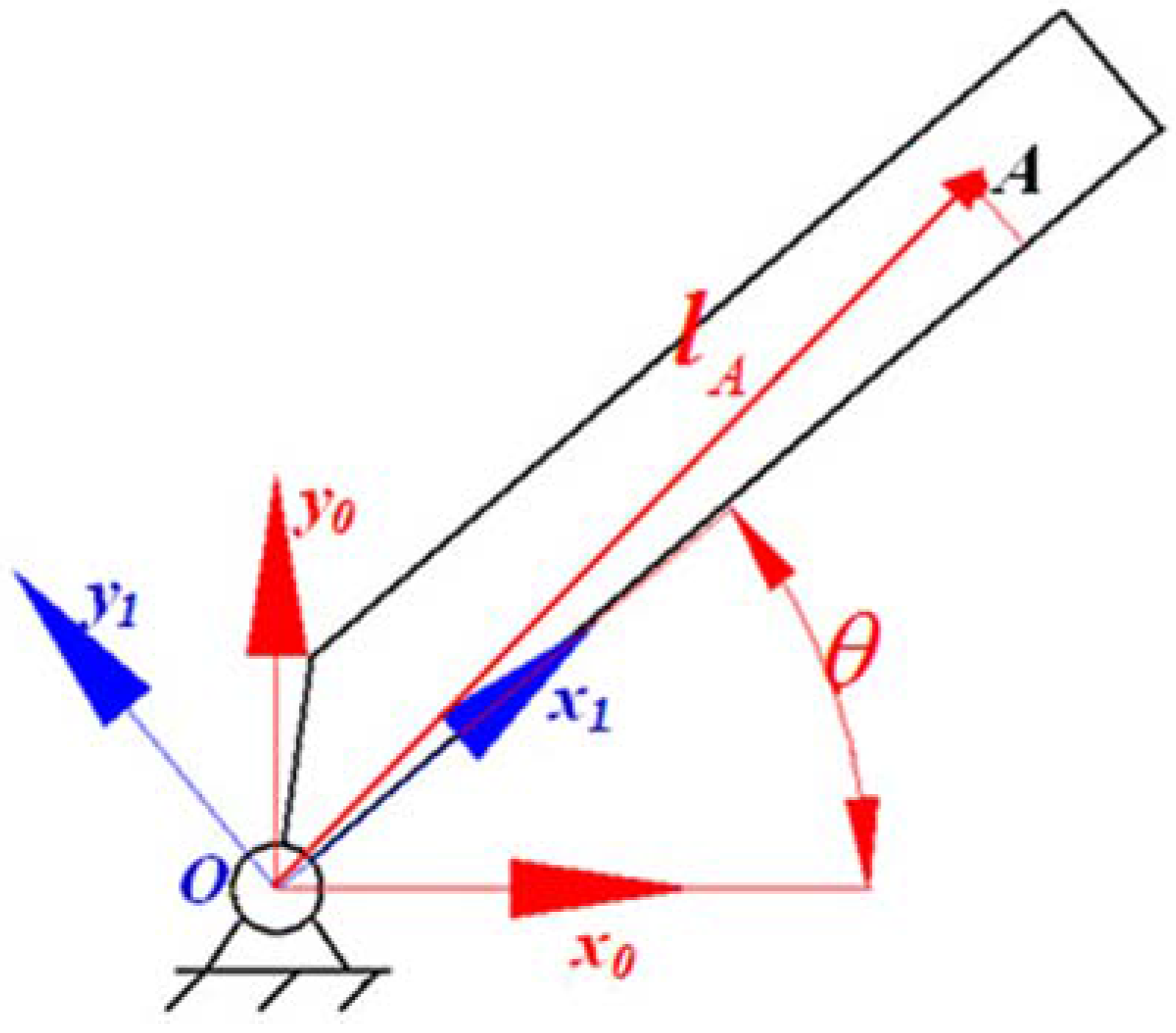
As in Figure 1, the cutting arm and the cutting head rotate along the z axis, the turntable rotates along the y axis, so the differential geometry in space SO(3) is needed. The differential geomery in SO(3) can be explained by the triangle function and the differential geometry on SO(2). Define the inertial frame Ox0y0 and the body frame which can rotate with the rod, as in Figure 2. Supposing that the axises from these two frames concide together at the initial moment, then the rod anticlockwise rotate along the point O, the projection of the axises of the body frame on the inertail frame can be expressed as the matrix type [22] as
the two elements in the two columns respect the projection of the axis of Ox1 and Oy1 in the inertial frame, the rotation matrix satisfies the following property

Figure 2.
The kinematic diagram of differential geometry.
According to Equation (1), the rotation matrix can be written as
in Equation (3), satisfy , is the unit matrix, is the skew matrix
The first order derivative of is
in Equation (5), . The properties of (2), (3), (5) avoid the triangle function that occurs in the following derivation. Equation (2) can be used to simplify the derivation process. The rotation matrix of the rod in plane can be expanded to be a three dimensional matrix which can express the rotation along the z axis in space. The relation between and is
if the rod rotates along the z axis, the vector on the z axis has no projection on the x and y axis, so the first two elements in the third column of the rotation matrix has no change. According to the Equation (5), the first order differential of the matrix is
the skew matrix in Equation (7) is
When the rod rotate along the y axis, the rotation matrix is
the projection of the unit vector on the y axis has no projection on the x and z axis, so the second column of is 1. The first order differential of is
the type of the skew matrix is
The above derivation gives the rotation matrix and the differential of the matrix of the rigid body in the three dimensional space which is rotated along the z axis and the y axis. In practice, the rod has some geometrical character, so the coordinate at any position in the rod needs to be defined. Supposing that the position vector of the point A (Figure 2) in Ox1y1 is , then the projection of point A in Ox0y0 after the rotation can be expressed as
The velocity vector of point A in Ox0y0 is
In addition, there are many sliding pairs, supposing that the coordinates of the two end points of the sliding pairs are , then the distance between the two points can be expressed as
4. The Pose and Attitude Analysis
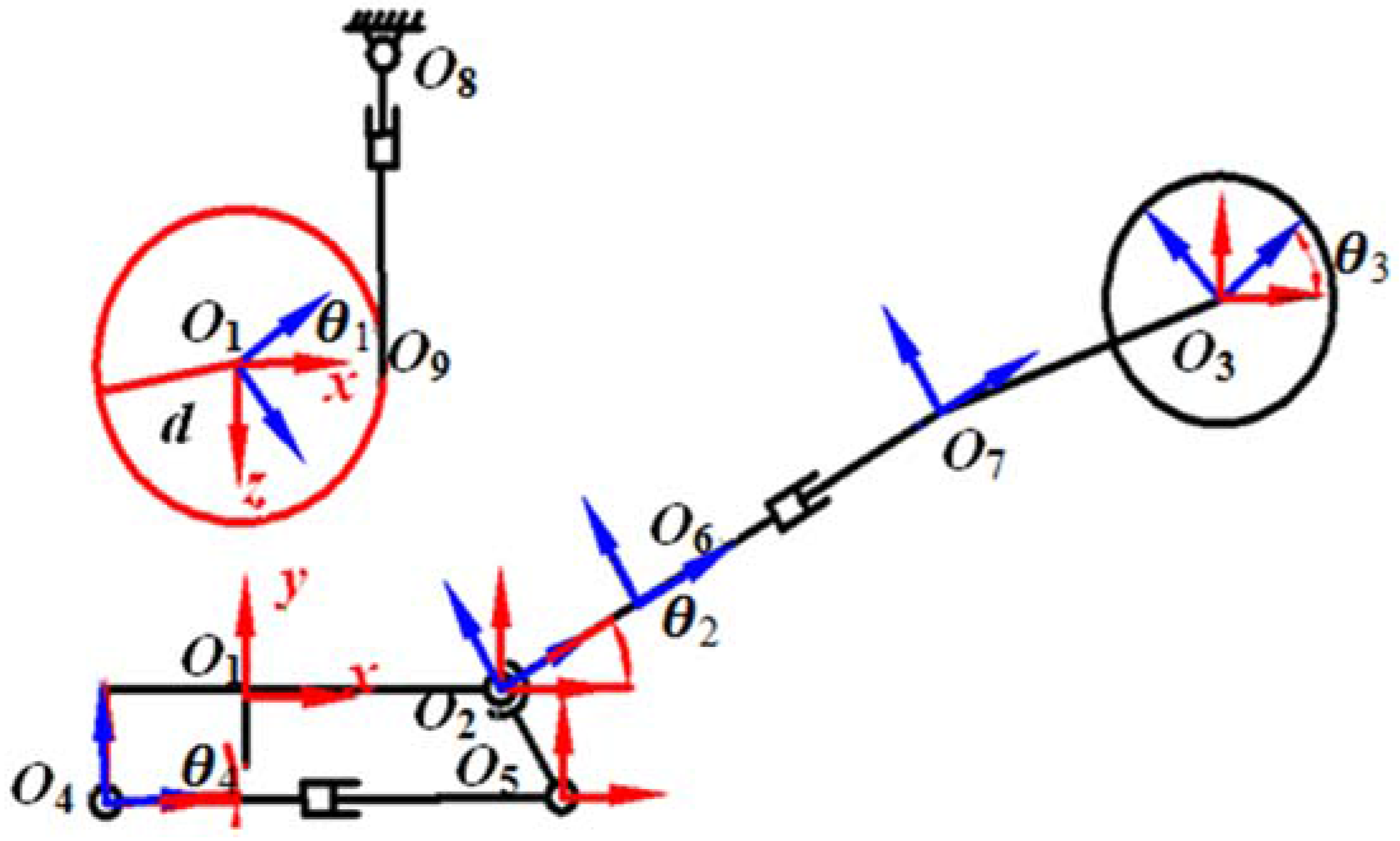
The geometry relation graph is shown in Figure 3. Supposing that the turntable is rotated along the frame O1, the cutting arm rotates along the frame O2, the cutting head rotates along the frame O3, the drive cylinder of the cutting arm is hinged with the turntable and the cutting arm by the point O4 and O5, respectively. The distance between the points O6 and O7 represents the length of the slip sleeve’s extending and shrinking. The driving cylinder of the turntable is fixed with the main engine by the point O8, the gear of the turntable is engaged with the rack by O9. Constructing the body frame and the inertial frame at these points respectively, the rotation direction of the body frames is all along the anticlockwise direction [23].

Figure 3.
The geometry relation of the heading machine.
According to the coupling relation of each motion component, the analysis of the motion is represented by the sequence from the cutting head to the cutting arm, then to the turntable. Define the position vector of the cutting tooth in the body frame at O3 to be , and the rotation angle of the cutting head along the z axis of the frame O3 to be , then the rotation matrix is as Equation (15). So the position vector of the cutting teeth in the inertial frame which is at the point of O3 is R3r1.
The relation of the slip sleeve and the cutting tooth is analyzed as follows. Define the coordinate vector of the O3 relative to the O7 to be r2, then the coordinate value of the cutting tooth relative to the frame O7 to be r2+R3r1. Define the distance between O6 and O7 is , and the x axis of the frame O6 and O7 are coincide with the line O6O7, so the coordinate of O7 relative to point O6 to be , then the position of the cutting tooth relative to the frame O6 is
Similarly, the distance between the points of O6 and O2 is , so the coordinate of O6 in the frame of O2 is , the coordinate of the cutting tooth in the frame O2 is
The about kinematics analysis of the cutting tooth is based on the body frame O2, when the cutting arm rotates along the z axis of the frame O2, the rotation matrix is
so the position of the cutting tooth in the inertial frame at the point O2 is
Define the distance between O2 and O1 to be , the position vector of O2 relative to frame O1 is , then the position vector of the cutting tooth in frame O1 is
Define the position of O5 in the body frame at point O2 to be , the point O5 rotate with the body frame at point O2, so the position vector of point O5 is , then the position of O5 in the frame at O1 is
Define the position vector of point O4 in the frame O1 to be , then the distance between the two points O4 and O5 can be expressed as
according to Equation (14), the distance can be calculated by the distance vector as Equation (23).
Dragging Equation (22) into Equation (23) to obtain the following equation
in Equation (24), . The Equation (24) is the pose and attitude relation between the length of the hydraulic rod O4 O5 and the rotation angle of the cutting arm. Supposing that the rotation angle of the rod rotate along the point is , the rotation matrix is
Define the initial position of the rod O4O5 to coincide with the x axis of the frame O4, the coordinate of the point O5 in the frame O1 after the rotation can be expressed as
With Equation (26), the rotation matrix can be derived. Equation (26) is the expression of the rotation motion of the hydraulic cylinder which accompany with the extending and shrinking of the hydraulic cylinder O4O5. When the turntable rotates along the y axis of frame O1, the rotation matrix is
According to Equation (20), the coordinate of the cutting tooth in the space is
5. The Velocity Analysis
Based on the pose and attitude relation, the velocity response of the cutting tooth can be derived by the differential calculation. The first order differential of the rotation matrixes are
, , , are the angular velocities of the turntable, the cutting arm, the cutting head and the hydraulic rod O4O5 respectively. Differentiate Equation (24), replace by the Equation (29), the relation between and is
The hydraulic rod is the actuator, the cutting arm is the driven part, so can be expressed as
the angular velocity of the cutting arm and the velocity of the rod O4O5 have a nonlinear relation. Differentiate Equation (26), the following relation can be obtained.
is the angular velocity of O4O5 rotate along O4, which can be expressed as
Differentiate Equation (28), the velocity of the cutting tooth is
bring Equation (29) into (34) to replace the first order differential part, the response of the velocity of the cutting tooth can be expressed as a neatly type.
the expressions of the parameters , , , are as follows.
if the pose and attitudes of each components of the system are known, , , , are constant values, so the velocity of the cutting tooth is the linear combination of .
6. The Acceleration Analysis of the Motion
The acceleration relations of the system are derived as follows. Firstly, the relation between the velocity of the extending and shrinking of the cylinder O4O5 and the angular acceleration of the cutting arm is derived. Differentiate Equation (30), the angular acceleration response of the cutting arm is
the expressions of the parameters and in Equation (37) are
the angular acceleration of the cutting arm has a complex nonlinear relation with the extending and shrinking acceleration and velocity of the hydraulic cylinder, also with the angular velocity of the cutting arm. The angular acceleration of the rod during the extending and shrinking is derived by the differentiate calculation of the Equation (32), as
are the values about the pose and attitudes, the expressions are
The acceleration response of the cutting tooth is derived by the differentiate calculation of the Equation (35), the result is
is the function about the pose and attitudes, which is expressed as follows. According to Equation (41), each motion of the components in the cutting part has an influence on the acceleration of the cutting tooth, and the motion has a high nonlinear character.
7. The Numerical Calculation Flow
The kinematic model has three parts: (24), (26) and (28) constitutes the pose and attitude relation, (31), (33) and (34) constitutes the velocity and angular velocity relation, (37), (39) and (41) constitutes the acceleration and angular acceleration relation. The kinematic model has a nonlinear character and recurrence connection, so the numerical solution is the only solving method. According to the recurrence relation, the calculation flow is confirmed as follows.
In the pose and attitude response, the Equation is a nonlinear equation which is implicit, the solution needs the help of the character of the rotation matrix to translate it to be a nonlinear equation system which can be solved by the numerical calculation method. According to Equation (3), the rotation matrix satisfies the following character:
the parameters in it are
, . Bring Equation (43) into (24) to obtain the nonlinear equation is
the expressions of the parameters are
the Equation (45) can be solved by the “fsolve” function in MATLAB [24]. With Equation (43), the Equation (26) can be translate to be the following type as
in Equation (47), . It is a linear equation with constant coefficient, so the results can be obtained directly.
8. The Simulation Results
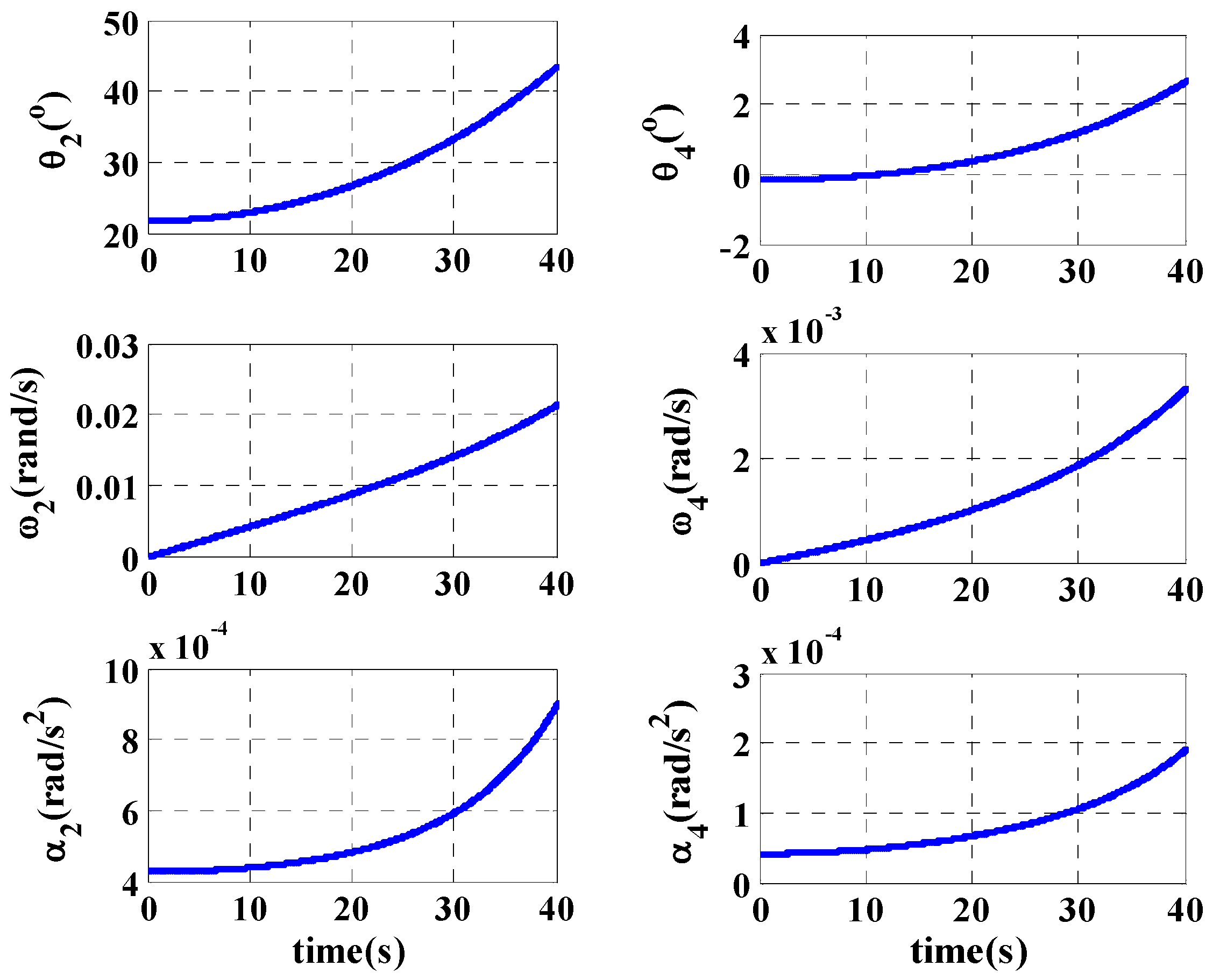
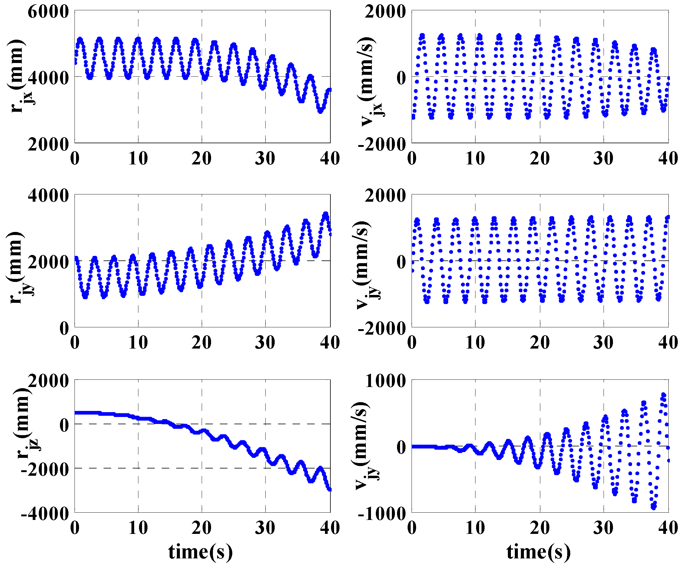
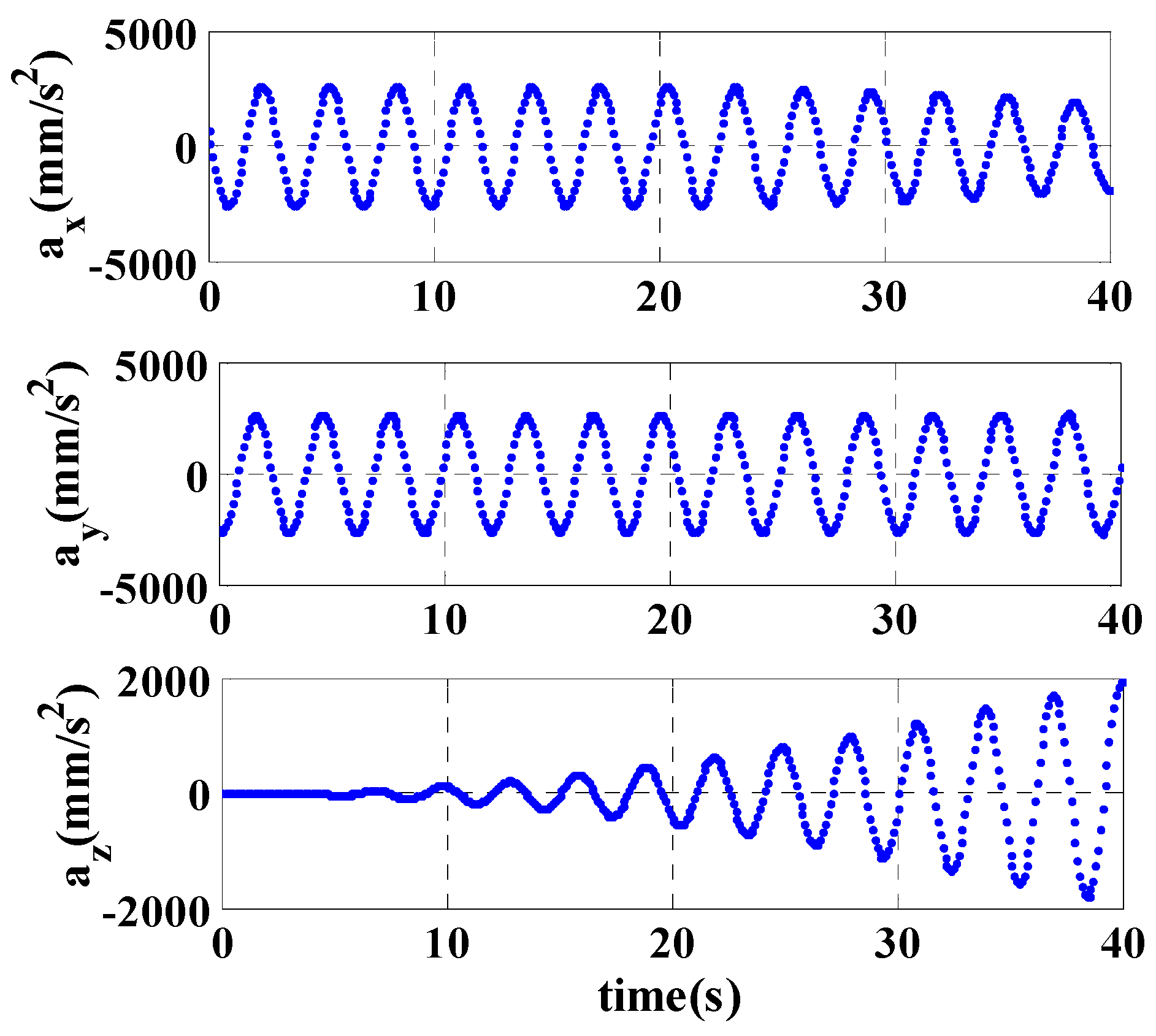
According to the structure of the heading machine, the main parameters are as follows. , mm. Setting the initial lengths to be , the initial attitudes are . The constant rotation angular velocity of the cutting head is set to . The acceleration of the dive cylinder of the turntable is 3.75 mm/s2, the initial and the end positions are 0 and 1500 mm respectively, the acceleration of the slip sleeve is 1 mm/s2, the initial and the end positions are 1538 mm and 1938 mm, respectively, the acceleration of the drive cylinder of the cutting arm is 0.5 mm/s2, the initial and the end positions are 2096 mm and 2296 mm, respectively. In the first 10 s, the turntable, the slip sleeve and the drive cylinder of the cutting arm are accelerated with their constant accelerations. Then they move with a constant velocity with the next 20 s, and decelerate within 10 s. The whole time of the simulation is 40 s. The simulation results of the kinematic parameters of the heading machine are shown in Figure 4, Figure 5, Figure 6 and Figure 7.
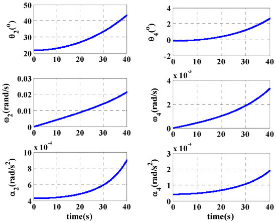
Figure 4.
The kinematics parameters of the cutting arm and drive cylinder.
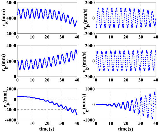
Figure 5.
The variation of the attitude and the velocity of the cutting tooth in space.
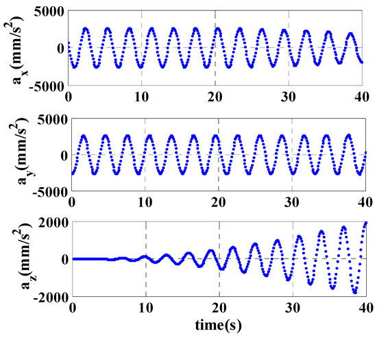
Figure 6.
The acceleration of the cutting tooth in space.
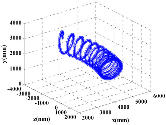
Figure 7.
The trajectory of the cutting tooth in space.
The variations of the angles, the angular velocities and the angular accelerations of the cutting arm and the drive cylinder of it are expressed in Figure 4. The curves are all smooth, which verifies the correctness of the Equations. With the rotation of the cutting arm, the drive cylinder has a small rotation angle, the angular velocities and the accelerations are all very small which meet the character of the heavy machine.
The variations of the attitude, the angular velocity and the angular acceleration are expressed in Figure 5 and Figure 6. According to Figure 5, the attitudes and the velocities of the cutting tooth which are projected on the x, y, z axis of the inertial frame are changed with the coupling motion of the turntable, the cutting arm, the slip sleeve and the cutting head. Their periodic waves are led by the motion of the cutting head, so the motion of the cutting tooth is the nonlinear coupling of all the motions parts. According to Figure 6, the variation of the acceleration of the cutting tooth on the x and y axis is small, which is mainly influenced by the pitching motion of the cutting arm and the slide motion of the slip sleeve. The variation on the z axis is obvious, which is mainly influenced by the yawn motion of the turntable. The trajectory of the cutting tooth in space is shown in Figure 7, the trajectory is a continuous loop curve which fixes the motion character of the cutting tooth in the practical application.
9. Summary and Prospects
In this paper, the kinematic model of the cutting part of the horizontal axis heading machine is established by the differential geometry method. In this modeling method, the triangle function is not realized and the expressions are simpler than in other methods. The kinematic relation between the linear parts and the cutting tooth are derived, the kinematic equation of the cutting tooth with high nonlinear character and the nonlinear response of other components is derived. A numerical calculation method is designed which can avoid the complex solution process. The correctness of the equations is testified by simulation. However, this paper uses differential equations and geometric concepts from linear algebra, but it does not use differential geometry of the type considered for kinematics of continuous media involving linear connections, torsion, curvature, etc., in reference [15] below. The pose and attitude response and the velocity and acceleration response offer a mathematical basis for the exploration of dynamics and the robotized exploration of the heading machine.
Acknowledgments
The exploration is supported by the Natural Science Foundation of China (11472058).
Author Contributions
Long Bai performed the derivation of the mathematical model and the simulation; Lu-han Ma performed the first part and the second part; Xin-sheng Ge analyzed the correctness of the simulation results.
Conflicts of Interest
The authors declare no conflict of interest.
References
- Guo, Y.F.; Zhagn, Y.Z. Kinematics analysis and computer simulation on longitudinal cutting head of roadheader. J. China Coal Soc. 2002, 27, 68–72. [Google Scholar]
- Guo, Y.F.; Zhang, Y.Z. Mathematical model and application of determining pick seat’s position for roadheader transverse cutting header. J. China Coal Soc. 2000, 25, 645–648. [Google Scholar]
- Zhao, L.J.; Liu, X.N. Horizontal swing movement parameters optimization design of longitudinal road header. J. China Coal Soc. 2012, 37, 2112–2117. [Google Scholar]
- Li, J.L.; Lian, Z.S. Kinematics analysis and carriage positions of roboticized roadheader. J. China Coal Soc. 2008, 33, 583–587. [Google Scholar]
- Chen, H.Y.; Ma, Y. Multi-body dynamics analysis on drilling manipulator of roadheader. J. China Coal Soc. 2013, 38, 1484–1489. [Google Scholar]
- Li, Y.G.; Song, Y.M. State of the art of robotics research based on modern differential geometry. China Mech. Eng. 2007, 18, 238–243. [Google Scholar]
- Luo, J.G.; Han, J.Y. Research method of mechanism based on differential geometry. J. Mach. Des. 2011, 28, 1–4. [Google Scholar] [CrossRef]
- Wang, Z.F.; Ma, S.G. A unified dynamic model for locomotion and manipulation of a snake-like robot based on differential geometry. Sci. China Inf. Sci. 2011, 41, 190–206. [Google Scholar] [CrossRef]
- Degn, X.J.; Lu, Z. Singularity analysis of overactuated parallel robots based on differential geometry. Chin. J. Mech. Eng. 2006, 42, 30–33. [Google Scholar]
- Ao, Y.H.; Chen, X. Dynamics and hybrid control of parallel mechanism based on differential geometry. China Mech. Eng. 2007, 18, 1339–1342. [Google Scholar]
- Sun, J.T.; Shi, S.C. Controller design of large space manipulator flexible joint using differential geometry algorithm. J. Harbin Eng. Univ. 2012, 33, 1371–1376. [Google Scholar]
- Lee, T. Computational Geomeric Mechanics and Control of Rigid Bodies; University of Michigan: Ann Arbor, MI, USA, 2008. [Google Scholar]
- Lee, T.; McClamroch Harris, N. A Lie group variational integrator for the attitude dynamics of a rigid body with application to the 3D pendulum. In Proceedings of the IEEE International Conference on Control Applications, Toronto, ON, Canada, 28–31 August 2005; pp. 962–967.
- Nordkvist, N.; Sanyal, A.K. A Lie group variational integrator for rigid body motion in SE(3) with applications to underwater vehicle dynamics. In Proceedings of the 49th IEEE Conference on Decision and Control, Atlanta, GA, USA, 15–17 December 2010; pp. 5414–5419.
- Clayton, J.D. Differential Geometry and Kinematics of Continua; World Scientific: Singapore, 2014. [Google Scholar]
- Dai, J.S. Screw Algebra and Lie Groups and Lie Algebras; Higher Education Press: Beijing, China, 2014. [Google Scholar]
- Dai, J.S. Geometrical Foundations and Screw Algebra for Mechanisms and Robotics; Higher Education Press: Beijing, China, 2014. [Google Scholar]
- Dai, J.S. Fundamentals and categorization of metamorphic mechanisms. Chin. J. Mech. Eng. 2005, 41, 7–12. [Google Scholar] [CrossRef]
- Dai, J.S. Historical Relation between Mechanisms and Screw Theory and the Development of Finite Displacement Screws. Chin. J. Mech. Eng. 2015, 51, 13–26. [Google Scholar] [CrossRef]
- Wang, D.L.; Wang, W. The Kinematic Differential Geometry and Saddle Synthesis of Linkages; China Machine Press: Beijing, China, 2015. [Google Scholar]
- Zhao, Y. The Mechanism Numerical Analysis and Synthesize; China Machine Press: Beijing, China, 2005. [Google Scholar]
- Liu, Y.Z.; Pan, Z.K.; Ge, X.S. Dynamics of Multibody Systems; Higher Education Press: Beijing, China, 2014; pp. 7–13. [Google Scholar]
- Saha, S.K. Introduction to Robotics; China Machine Press: Beijing, China, 2014; pp. 101–108. [Google Scholar]
- Ding, L.J.; Cheng, Q.Y. Numerical Calculation Method; Higher Education Press: Beijing, China, 2011; pp. 283–285. [Google Scholar]
© 2016 by the authors; licensee MDPI, Basel, Switzerland. This article is an open access article distributed under the terms and conditions of the Creative Commons Attribution (CC-BY) license (http://creativecommons.org/licenses/by/4.0/).


