Fixed Order Controller for Schur Stability

Abstract

If the characteristic polynomial of a discrete-time system has all its roots in the open unit disc of the complex plane, the system is called Schur stable. In this paper, the Schur stabilization problem of closed loop discrete-time system by affine compensator is considered. For this purpose, the distance function between the Schur stability region and the affine controller subset is investigated.

1. Introduction

A polynomial $p(s)=s^n+a_n{s}^{n-1}+\cdots +a_{2}s+a_1$ with real coefficients is called Schur stable if all its roots lie in the open unit disc of the complex plane. Schur stability is very important in the investigation of discrete-time systems. One of the ways to investigate of Schur stability is the use of the well-known bilinear transformation between the open left half plane and the open unit disc. By using this transformation, the Schur stability problem of a given system can be transformed into Hurwitz stability problem of transformed polynomial (Recall that a system is called Hurwitz stable if all roots of its characteristic polynomial belong to the open left half plane) [1,2,3,4,5].

Each polynomial $p(s)$ corresponds to an n-dimensional vector $p={(a_1,a_2,\dots ,a_n)}^T\in {\mathbb{R}}^n$. The vector p is called stable if the corresponding monic polynomial $p(s)$ is Schur stable. Denote the set of such stable vectors by $\mathcal{D}$. In other words $\mathcal{D}=\{{(a_1,a_2,\dots ,a_n)}^T\in {\mathbb{R}}^n:$ The polynomial $p(s)=s^n+a_n{s}^{n-1}+\cdots +a_{2}s+a_1$ is Schur stableg}. It is well-known that the set $\mathcal{D}$ is non-convex for $n>2$ and open. The closed convex hull of $\mathcal{D}$ is a polytope [6,7].

Many stabilization problems of discrete-time systems by feedback controller can be reduced to the following: Consider a family

$$p(s,c)=p_0(s)+c_1{p}_1(s)+c_2{p}_2(s)+\cdots +c_l{p}_l(s)$$

(1)

where $\mathrm{degree}(p_0)=n$, $\mathrm{degree}(p_i)<n$ $(i=1,2,\dots ,l)$ and $l<n$. Find l-dimensional vector $c={(c_1,c_2,\dots ,c_l)}^T\in {\mathbb{R}}^l$ such that the corresponding polynomial $p(s,c)$ is Schur stable. In this case, the vector c is called a stabilizing vector. The polynomial equality (1) can be written in vector-matrix form as follows. Consider column vectors $p^0,p^1,\dots ,p^l$ where $p^0$ corresponds to $p_0(s)$ and $p^i$ $(i=1,2,\dots ,l)$ correspond to $p_i(s)$ with the property that added zero component have dimension n. For instance, assume $p_0(s)=s^4+5s^3+2s^2+s+1$ and $p_1(s)=2s^3+s$. Then $p^0={(1,1,2,5)}^T$, $p^1={(0,1,0,2)}^T$.

Define $n\times l$ dimensional matrix $A=\left[p^1,p^2,\dots ,p^l\right]$. Then relation (1) can be written in vector-matrix form as follows:

$$p(c)=Ac+p^0.$$

(2)

The stabilization problem is the determination of a parameter $c\in {\mathbb{R}}^l$ with the property that $Ac+p^0\in \mathcal{D}$, namely, find conditions under which $\mathcal{P}\cap \mathcal{D}\ne \varnothing$, where $\mathcal{P}=\{Ac+p^0:c\in {\mathbb{R}}^l\}$ is an affine subset of ${\mathbb{R}}^n$.

In [8,9] for determination of a stabilizing parameter $c,$ the method of random generation of stable vectors and stable segments are suggested. In [10], for stabilization of continuous-time systems part of specially selected parameters are chosen randomly and another part deterministically. The combination of sum of square and linear matrix inequalities techniques for approximation of the set of stabilizing controllers for continuous time system has been considered in [11]. For such systems, a linear programming approach is considered in [12]. Stabilizing controls based on matrix inequalities have been considered in [13,14,15].

In this paper, we consider the problem of existence of an affine controller for discrete-time systems. In Section 2, we give a simple condition for the existence of a stabilizing parameter c. In Section 3, the Euclidean distance between the sets $\mathcal{D}$ and $\mathcal{P}$ is investigated, from which some existence and nonexistence conditions are obtained.

2. Rank Condition

In this section we give condition for the existence and evaluating of a stabilizing parameter c and corresponding examples. The condition is based on Rouché-Capelli theorem [16]. Without loss of generality we can assume that $p^1,\dots ,p^l$ are linearly independent. If these vectors are linearly dependent then number of uncertain parameters $c_1,c_2,\dots ,c_l$ will be reduced.

Proposition 1. 

Assume that the vectors $p^1,p^2,\dots ,p^l$ are linearly independent. Then there exists a stabilizing parameter $c\in {\mathbb{R}}^l$ if and only if there exists $q\in \mathcal{D}$ such that

$$\mathrm{rank}\left[p^1,p^2,\dots ,p^l,q-p^0\right]=l.$$

(3)

Proof. 

There exists a stabilizing vector if and only if there exist $q\in \mathcal{D}$, $c\in {\mathbb{R}}^l$ such that

$$Ac+p^0=q \mathrm{or} Ac=q-p^0.$$

(4)

By Rouché-Capelli theorem, for given $q\in \mathcal{D}$, the linear system (4) on unknown vector c has unique solution $c\in {\mathcal{R}}^l$ if and only if

$$\mathrm{rank}\left[p^1,p^2,\dots ,p^l,q-p^0\right]=\mathrm{rank}\left[p^1,p^2,\dots ,p^l\right]=l.$$

□

Corollary 2. 

Assume that $p^1,p^2,\dots ,p^l$ are linearly independent and

$$\mathrm{rank}\left[p^0,p^1,\dots ,p^l\right]=l.$$

Then there exists a stabilizing parameter $c\in {\mathbb{R}}^l$.

Proof. 

In Proposition 1, take $q=0$ which corresponds to the Schur stable polynomial $p(s)=s^n$. Then (4) is satisfied for $q=0\in \mathcal{D}$.   □

Example 1. 

Consider the proper plant

$$G(s)=\frac{s^2+0.8s-0.5}{s^4+0.7s^3+0.16s^2-0.67s+0.2}$$

with PID controller ${\displaystyle C(s)=\frac{c_3{s}^2+c_{2}s+c_1}{s}}$.

The closed loop characteristic polynomial is

$$\begin{array}{ccc}\hfill p(s,c)& =& (s^2+0.8s-0.5)(c_3{s}^2+c_{2}s+c_1)+s(s^4+0.7s^3+0.16s^2-0.67s+0.2)\hfill \\ & =& s^5+0.7s^4+0.16s^3-0.67s^2+0.2s+c_1(s^2+0.8s-0.5)+\hfill \\ & & c_2(s^3+0.8s^2-0.5s)+c_3(s^4+0.8s^3-0.5s^2).\hfill \end{array}$$

The polynomial $p_0(s)=s^5+0.7s^4+0.16s^3-0.67s^2+0.2s$ is not Schur stable. Here

$$\begin{array}{ccc}{p}^0={(0,0.2,-0.67,0.16,0.7)}^T,\hfill & p^1={(-0.5,0.8,1,0,0)}^T,\hfill & p^2={(0,-0.5,0.8,1,0)}^T,\hfill \\ p^3={(0,0,-0.5,0.8,1)}^T.\hfill & \end{array}$$

The vectors $p^1$, $p^2$, $p^3$ are linearly independent, whereas $p^0$, $p^1$, $p^2$ and $p^3$ are linearly dependent:

$$p^0+0.4p^2-0.7p^3=0.$$

Therefore, by Corollary 2 the vector $c={(0,0.4,-0.7)}^T$ is a stabilizing parameter.

Example 2. 

Consider the fourth-order polynomial family

$$\begin{array}{ccc}p(s,c)& =& \hfill s^4-1.8s^3+1.86s^2-0.52s+c_1(s^3-3s^2-s-0.4)+\\ & & \hfill c_2(s^2-s-0.5)+c_3(s^3-s^2+0.5s-0.6)\end{array}$$

where the polynomial $p_0(s)=s^4-1.8s^3+1.86s^2-0.52s$ is not Schur stable. For this family, corresponding vectors are

$$\begin{array}{ccc}{p}^0={(0,-0.52,1.86,-1.8)}^T,\hfill & p^1={(-0.4,-1,-3,1)}^T,\hfill & p^2={(-0.5,-1,1,0)}^T,\hfill \\ p^3={(-0.6,0.5,-1,1)}^T\hfill & \end{array}$$

and the vectors $p^1$, $p^2$, $p^3$ are linearly independent. For the Schur stable polynomial $q(s)=s^4-2.1s^3+2.16s^2-1.02s+0.1$, the vectors $p^0-q$ $p^1$, $p^2$, $p^3$ are linearly dependent, where $q={(0.1,-1.02,2.16,-2.1)}^T$. We have $0.1p^1+0.2p^2-0.4p^3=q-p^0$ and by Proposition 1 the vector $c={(0.1,0.2,-0.4)}^T$ is a stabilizing parameter.

3. Schur-Szegö Parameters and Polynomial Optimization

Schur-Szegö parameters [17] or reflection coefficients are widely used in the stability problems of discrete time systems. Let us briefly recall these coefficients. In [18], for $k_i\in \mathbb{R}$ ($i=1,2,\dots ,n$) the reflection map $f={(f_1,f_2,\dots ,f_n)}^T$ is defined recursively:

$${(f_1,f_2,\dots ,f_n)}^T=R_n(k_n)\left[\begin{array}{c}{0}^T\\ R_{n-1}(k_{n-1})\end{array}\right]\dots \left[\begin{array}{c}{0}^T\\ R_1(k_1)\end{array}\right]\left[\begin{array}{c}0\\ 1\end{array}\right]$$

where $R_j(k_j)=I_{j+1}+k_j{E}_{j+1}$, $I_j$ is $j\times j$ unit matrix and, $E_j$ is $j\times j$ dimensional, defined by

$$E_j=\left[\begin{array}{ccc}0& \dots & 1\\ ⋮& \ddots & ⋮\\ 1& \dots & 0\end{array}\right].$$

In the above formula, the first zero is n-dimensional, whereas the last is one-dimensional. The above formula gives

for $n=3$,

$$\begin{array}{ccc}{f}_1(k_1,k_2,k_3)=-k_3,\hfill & f_2(k_1,k_2,k_3)=-k_1{k}_2{k}_3+k_1{k}_3-k_2,\hfill & f_3(k_1,k_2,k_3)=k_1{k}_2+k_2{k}_3-k_1,\hfill \end{array}$$

for $n=4$,

$$\begin{array}{c}{f}_1(k_1,k_2,k_3,k_4)=-k_4,\hfill \\ f_2(k_1,k_2,k_3,k_4)=-k_1{k}_2{k}_4-k_2{k}_3{k}_4+k_1{k}_4-k_3,\hfill \\ f_3(k_1,k_2,k_3,k_4)=k_1{k}_2{k}_3{k}_4-k_1{k}_2{k}_3-k_1{k}_3{k}_4+k_1{k}_3+k_2{k}_4-k_2,\hfill \\ f_4(k_1,k_2,k_3,k_4)=k_1{k}_2+k_2{k}_3+k_3{k}_4-k_1\hfill \end{array}$$

and so on. The polynomial $p(s)=s^n+f_n{s}^{n-1}+\cdots +f_{2}s+f_1$ is Schur stable if and only if $|k_i|<1$ for all $i=1,2,\dots ,n$. The map $f(k)$ between the reflection vector $k={(k_1,k_2,\dots ,k_n)}^T$ and the coefficient vector $p={(f_1,f_2,\dots ,f_n)}^T$ is multilinear. By known property of multilinear maps [1] (p. 435) namely, the convex hull of the image of a multilinear map defined on a box Q is equal the convex hull of the images of vertices of Q. In [6], it has been proven that there is no need to take all vertices of Q, the convex hull of the image of f is a polytope, whose vertices correspond to the $n+1$ polynomials for which zeros are equal to $-1$ or 1.

By using Schur-Szegö parameters, we can generate an arbitrary number of Schur stable polynomials: For this purpose it is sufficient to choose any vector $k=(k_1,k_2,\dots ,k_n)\in (-1,1)\times (-1,1)\times \cdots \times (-1,1)$ and find the image $f(k)$. The obtained vector $f(k)$ is stable.

Consider the distance function between the sets $\mathcal{P}$ and ${\mathcal{D}}_n$. Recall that $\mathcal{P}$ is closed affine set whereas ${\mathcal{D}}_n$ is an open set. We show that the distance function between them is n-variable polynomial with total degree $2n$. The variables of this polynomial are Schur-Szegö parameters $k=(k_1,k_2,\dots ,k_n)\in {(-1,1)}^n$. We consider the minimization of this polynomial over the closed cube ${[-1,1]}^n$ and use the Bernstein expansion for the outer approximation of the range.

Consider the number

$$\alpha :=\underset{c\in {\mathbb{R}}^l,k\in {[-1,1]}^n}{inf}\parallel Ac+p^0-f(k_1,k_2,\dots ,k_n)\parallel$$

(5)

where $c={(c_1,c_2,\dots ,c_l)}^T$, A is $n\times l$ matrix with column vectors $p^1,p^2,\dots ,p^l$, i.e., $A=\left[p^1,p^2,\dots ,p^l\right]$, $\parallel x\parallel$ is the Euclidean norm of x, f is multilinear reflection map.

Theorem 3. 

The equality

$$\alpha =\underset{k\in {[-1,1]}^n}{min}\parallel A{(A^{T}A)}^{-1}{A}^T(f(k_1,k_2,\dots ,k_n)-p^0)+p^0-f(k_1,k_2,\dots ,k_n)\parallel$$

(6)

is satisfied.

Proof. 

Write

$$\alpha =\underset{k}{inf}\underset{c}{inf}\parallel Ac-y\parallel =\underset{k}{inf}F(k_1,k_2,\dots ,k_n)$$

where ${\displaystyle y=f(k_1,k_2,\dots ,k_n)-p^0,F(k_1,k_2,\dots ,k_n)=\underset{c}{inf}\parallel Ac-y\parallel }$.

Define l-dimensional subspace $W=\mathrm{span}\{p^1,p^2,\dots ,p^l\}$. Then $F(k_1,k_2,\dots ,k_n)$ is the distance from the point y to W. By the well-known theorem of functional analysis [19], the nearest point $\widehat{y}\in W$ exists and satisfies $(y-\widehat{y})\perp W$, where $x\perp W$ means $⟨x,w⟩=0$ for all $w\in W$ and the symbol $⟨·,·⟩$ stands for the scalar product.

We have

$$(y-\widehat{y})\perp p^i,{(p^i)}^T(y-\widehat{y})=0(i=1,2,\dots ,l)$$

or

$$A^T(y-\widehat{y})=0,A^{T}y=A^T\widehat{y}.$$

Since $\widehat{y}\in W$, where $\widehat{y}=c_1^{*}{p}^1+c_2^{*}{p}^2+\cdots +c_l^{*}{p}^l=A{c}^{*}$, where $c^{*}={(c_1^{*},c_2^{*},\dots ,c_l^{*})}^T$, we have

$$A^{T}y=A^{T}A{c}^{*}.$$

The matrix $A^{T}A$ is nonsingular. By contradiction, assume that there exists nonzero $x\in {\mathbb{R}}^l$ such that $A^{T}Ax=0$. Then

$${\parallel Ax\parallel }^2=⟨Ax,Ax⟩={(Ax)}^{T}Ax=x^T{A}^{T}Ax=x^{T}0=0$$

and $Ax=0$. The last equality contradicts to the linear independence of $p^1,p^2,\dots ,p^l$. Therefore $c^{*}={(A^{T}A)}^{-1}{A}^{T}y$ and

$$\begin{array}{ccc}F(k_1,k_2,\dots ,k_n)\hfill & =& {\displaystyle \underset{c}{inf}\parallel Ac-y\parallel =\parallel A{c}^{*}-y\parallel }\hfill \\ & =& \parallel A{(A^{T}A)}^{-1}{A}^T(f(k_1,k_2,\dots ,k_n)-p^0)-(f(k_1,k_2,\dots ,k_n)-p^0)\parallel \hfill \end{array}$$

and the equality (6) follows.   □

Proposition 4. 

If $\alpha >0$ then there is no stabilizing parameter c.

If $\alpha =0$ then $\mathcal{P}\cap \overline{\mathcal{D}}\ne \varnothing$ and either there exists a stabilizing parameter c or there is no stabilizing parameter c, but there exists a parameter c such that $p(s,c)$ is marginally stable, i.e., has all roots in the closure of the open unit disc. It should be noted that the last case is rather a pathological than a typical one.

Consider the number

$${\alpha }^2=\underset{k\in {[-1,1]}^n}{min}{F}^2(k_1,k_2,\dots ,k_n).$$

The function $(k_1,k_2,\dots ,k_n)\to F^2(k_1,k_2,\dots ,k_n)$ is a multivariable polynomial defined on the box ${[-1,1]}^n$. The range $F^2(k_1,k_2,\dots ,k_n)$ can be estimated by the Bernstein expansion. Let us briefly describe this expansion for n-variate polynomials [20].

An n-variate polynomial $v(x)$ is defined as

$$v(x)=\sum _{L\le N}{a}_L{x}^L(x\in {\mathbb{R}}^n),$$

(7)

where $L=(i_1,i_2,\dots ,i_n)$, $N=(s_1,s_2,\dots ,s_n)$, $x^L=x_1^{i_1}{x}_2^{i_2}\cdots x_n^{i_n}$ and

$$L\le n\iff 0\le i_j\le s_j(j=1,2,\dots ,n).$$

The Lth Bernstein polynomial of degree d is defined by

$$B_{N,L}(x)=b_{s_1,i_1}(x_1)\cdots b_{s_n,i_n}(x_n)(x\in {\mathbb{R}}^n)$$

where $b_{s,i}(t)=\left(\genfrac{}{}{0pt}{}{n}{i}\right)t^i{(1-t)}^{n-i}$. The transformation of a polynomial from its power from (7) into its Bernstein form result in

$$v(x)=\sum _{L\le N}{v}_L(U)B_{N,L}(x),$$

where the Bernstein coefficients $v_L(U)$ of v over the n-dimensional unit box $U=[0,1]\times \cdots \times [0,1]$ are given by

$$v_L(U)=\sum _{j\le N}\frac{\left(\genfrac{}{}{0pt}{}{L}{J}\right)}{\left(\genfrac{}{}{0pt}{}{N}{J}\right)}{a}_J(L\le N).$$

Here $\left(\genfrac{}{}{0pt}{}{N}{L}\right)$ is defined as $\left(\genfrac{}{}{0pt}{}{s_1}{i_1}\right)\cdots \left(\genfrac{}{}{0pt}{}{s_n}{i_n}\right)$.

Let

$$\begin{array}{c}\underline{m}=min\{v(x):x\in U\},\hfill \\ \overline{m}=max\{v(x):x\in U\},\hfill \\ \alpha =min\{v_L(U):L\le N\},\hfill \\ \beta =max\{v_L(U):L\le N\}.\hfill \end{array}$$

Theorem 5. 

[20] The following inequalities

$$\alpha \le \underline{m}\le \overline{m}\le \beta$$

are satisfied.

Theorem 5 gives outer approximation of the range of $v(x)$ over the unit box U.

In order to obtain the Bernstein coefficients and bounds over an arbitrary box D rather the unit box U, the box D should be affinely mapped onto U. To obtain convergent bounds for the range of the polynomial (7) over the box U, the box U should be divided into small boxes.

If $\alpha >0$ ($\beta <0$) then the polynomial is positive (negative) on U. If $\alpha \le 0$, $\beta \ge 0$ then by the bisection in the chosen coordinate direction, the box U is divided into two boxes. A new box on which the inequality $\alpha >0$ or $\beta <0$ is satisfied should be eliminated, since our polynomial has constant sign on this box. Otherwise, the box should be divided into two new boxes.

If at some step of the Bernstein expansion the lower bound is positive then ${\alpha }^2>0$ and $\alpha >0$ and there is no stabilizing c. If this is not the case, an additional investigation on existence is required.

Taking into account the definition of α and Proposition 4, we can suggest the following algorithm for a stabilizing vector.

Algorithm 6. 

(1)

Given family (1), explicitly calculate the multivariable polynomial $F^2(k_1,k_2,\dots ,k_n)$.

(2)

Calculate step-by-step the Bernstein coefficients for the function $F^2$ over the box ${[-1,1]}^n$. If at some step, the minimal Bernstein coefficient is positive then stop, there is no stabilizing parameter c.

(3)

If after a sufficiently large number of steps the lower Bernstein coefficient remains negative, then stop and carry out an additional test for the existence of a stabilizing vector c. A cycling of the calculation indicates the existence of a stabilizing parameter. In this case, we can proceed to a random search if number of remaining boxes is small. For example, choose the center point $k^{*}$ of a remaining box, calculate $c^{*}={(A^{T}A)}^{-1}(f(k^{*})-U^0)$ and test $c^{*}$ for a stabilizing vector, i.e., test Schur stability of $p(s,c^{*})$. Alternatively, the gradient minimization method of the smooth function $F^2$ could be applied.

Example 3. 

Consider stabilizing problem for the following polynomial family:

$$p(s,c)=s^5+(c_1+c_2)s^4+(-2+3c_1-c_2)s^3+(-2c_1+4c_2)s^2+(1-c_1-5c_2)s-1+c_1-3c_2.$$

The matrix A (see (2)) and the vector $p^0$ are

$$A=\left[\begin{array}{cc}1& -3\\ -1& -5\\ -2& 4\\ 3& -1\\ 1& 1\end{array}\right],p^0=\left[\begin{array}{c}-1\\ 1\\ 0\\ -2\\ 0\end{array}\right]$$

and we have

$$\begin{array}{ccc}{F}^2(k_1,k_2,k_3,k_4,k_5)\hfill & =\hfill & \parallel A{(A^{T}A)}^{-1}{A}^T(f(k_1,k_2,k_3,k_4,k_5)-p^0)+p^0-f(k_1,k_2,k_3,k_4,k_5){\parallel }^2\hfill \\ & =\hfill & {\displaystyle \frac{83}{192}{k}_1^2{k}_2^2{k}_4^2{k}_5^2+\frac{9}{16}{k}_1^2{k}_3^2{k}_4^2{k}_5^2+\cdots +\frac{11}{8}{k}_1^2{k}_2{k}_3{k}_4^2{k}_5^2-\frac{61}{24}{k}_1{k}_2{k}_3^2{k}_4^2{k}_5+}\hfill \\ & & {\displaystyle \cdots +\frac{9}{16}{k}_2^2{k}_3^2{k}_4^2-\frac{11}{16}{k}_1^2{k}_3^2{k}_5-\frac{11}{16}{k}_1^2{k}_3{k}_4^2-\frac{7}{16}{k}_1^2{k}_3{k}_5^2+\cdots -\frac{1}{2}{k}_1{k}_2{k}_5}\hfill \\ & & {\displaystyle -\frac{9}{4}{k}_1{k}_2{k}_4-\frac{29}{24}{k}_1{k}_3{k}_5-\frac{9}{4}{k}_2{k}_3{k}_4-\frac{29}{24}{k}_2{k}_4{k}_5-\frac{31}{16}{k}_2{k}_3{k}_5-\frac{1}{2}{k}_5+\frac{5}{3}.}\hfill \end{array}$$

When Algorithm 6 is applied, 477 subboxes remained at the end of 1000 steps after 48 seconds. Consider one of these subboxes:

$$[0.625,0.75]\times [0.625,0.75]\times [0.875,1]\times [0.5,0.75]\times [0.5,0.75].$$

The center of this subbox is $k^{*}={(0.6875,0.6875,0.9375,0.625,0.625)}^T$ and the corresponding $c^{*}$ can be calculated as

$$c^{*}={(A^{T}A)}^{-1}(f(k^{*})-U^0)={(0.992173,0.241873)}^T.$$

The corresponding polynomial $p(s,c^{*})$ is Schur stable, i.e., $c^{*}$ is a stabilizing vector.

Example 4 

(There is no stabilizing c) Consider the family

$$p(s,c)=s^5+(c_1+c_2)s^4+(0.9-3c_1-2c_2)s^3+(-3c_1-4c_2)s^2+(-1.8-3c_1+6c_2)s-1.1+c_1-c_2.$$

Here $p^0={(-1.1,-1.8,0,0.9,0)}^T$, $p^1={(1,-3,-3,-3,1)}^T$ and $p^2={(-1,6,-4,-2,1)}^T$. The polynomial $F^2$ is 5-variate quadratic polynomial. We apply the Bernstein expansion, splitting-elimination procedure and after 698 steps (during $34.5$ second) conclude that $F^2>0$ on ${[-1,1]}^5$. Therefore, there is no stabilizing parameter c.

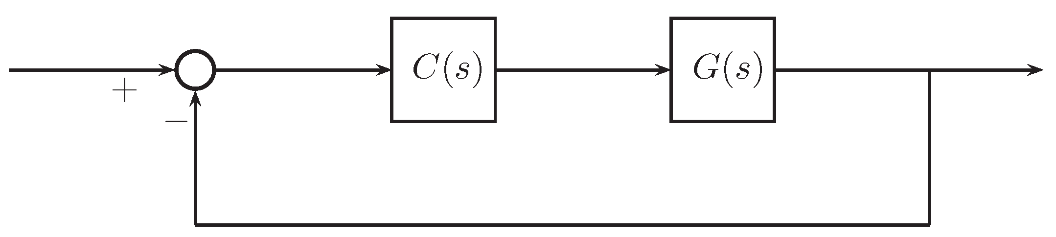
Example 5. 

Let the control system shown in the Figure 1 be given. Assume that transfer function and controller are

$$G(s)=\frac{s^3-0.3s^2-0.1s+1.6}{s^5+0.4s^4-1.8s^3-0.7s^2+0.2s-0.6}\mathrm{and}C(s)=\frac{c_3{s}^2+c_{2}s+c_1}{s}.$$

Figure 1. A closed loop system for Example 5.

The characteristic polynomial of the closed-loop system becomes

$$\begin{array}{ccc}\hfill p(s,c)& =& s^6+(0.4+c_3)s^5+(-1.8+c_2-0.3c_3)s^4+(-0.7+c_1-0.3c_2-0.1c_3)s^3+\hfill \\ & & (0.2-0.3c_1-0.1c_2+1.6c_3)s^2+(-0.6-0.1c_1+1.6c_2)s+1.6c_1\hfill \end{array}$$

Let $c_3=1$. We apply Algorithm 6, part 2 and after 3726 steps conclude that there is no stabilizing parameter c.

Let $c_3=0.5$. In this case, Algorithm 6 applied to the problem of stabilization does not give a negative result after 20000 steps with 6538 subboxes, and

$$[0.9375,1]\times [0.1875,0.25]\times [0,0.125]\times [0,0.125]\times [0,0.125]\times [0.625,0.75]$$

is one of them. The center of this subbox is $k^{*}={(0.96875,0.21875,0.0625,0.0625,0.0625,0.6875)}^T$ and calculations give $c^{*}={(0.05756065,0.91839451,0.5)}^T$. Since the polynomial $p(s,c^{*})$ is Schur stable, $c^{*}$ is a stabilizing vector.

Remark 1. 

Here, we indicate advantages and disadvantages of our results given in this paper. Firstly, note that Proposition 1 has a simple form. On the other hand the results existing in the literature on the existence and evaluation of Schur stable element in an affine polynomial family are mainly random search methods (see [9] and references therein). Algorithm 6 gives an answer when there does not exist a stabilizing parameter; however, it gives a useful hint as to whether such a parameter exists. The main setback of Algorithm 6 is that high-dimensional systems require long calculations.

4. Conclusions

In this paper, the stabilization problem of closed-loop discrete-time systems by affine compensator is considered. A condition based on linear dependence of system vectors is obtained. The distance function between the Schur stability region and the affine controller subset is investigated. The optimal value of this function gives the conditions for stabilizability of the system.