Abstract
This manuscript focuses attention on new exact solutions of the system of equations for the ion sound wave under the action of the ponderomotive force due to high-frequency field and for the Langmuir wave. The extended trial equation method (ETEM), which is one of the analytical methods, has been handled for finding exact solutions of the system of equations for the ion sound wave and the Langmuir wave. By using this method, exact solutions including the rational function solution, traveling wave solution, soliton solution, Jacobi elliptic function solution, hyperbolic function solution and periodic wave solution of this system of equations have been obtained. In addition, by using Mathematica Release 9, some graphical simulations were done to see the behavior of these solutions.
1. Introduction
The survey of new exact solutions for the ion sound wave and the Langmuir wave has a highly important position among the scientists. Many authors have worked on the Langmuir solitons. Degtyarev et al. have presented some properties of Langmuir solitons [1]. Then, they have examined the Langmuir wave energy dissipation [2]. Some authors have obtained the numerical simulations of Langmuir collapse [3,4,5,6]. Benilov has demonstrated the stability of solitons by using the Zakharov equation which identifies the interaction between Langmuir and ion-sound waves [7]. Zakharov et al. have exhibited the modeling of Langmuir turbulence [8]. Dyachenko et al. have calculated computer simulations of Langmuir collapse [9]. Rubenchik et al. have studied strong Langmuir turbulence in laser plasma [10]. Musher et al. have submitted weak Langmuir turbulence [11]. In addition, some authors have focused on Langmuir waves [12,13,14]. Dodin et al. have tackled Langmuir wave evolution in nonstationary plasma [15]. Zavlavsky et al. have considered spatial localization of Langmuir waves [16]. In addition, Langmuir wave spectral energy densities have been derived from the electric field and compared to the weak turbulence results by Ratcliffe et al. [17].
We consider the system of equations for the ion sound wave under the action of the ponderomotive force due to high-frequency field and for the Langmuir wave [18]:
where is the normalized electric field of the Langmuir oscillation and is the normalized density perturbation. The spatial variable and the time variable are also normalized appropriately [18]. The system of Equation (1) for the ion sound and Langmuir waves has been submitted by Zakharov [19]. Recently, this system has been investigated by some authors [20,21,22,23,24,25,26].
In this study, the basic interest is to constitute new exact solutions of the system of equations for the ion sound and Langmuir waves via extended trial equation method (ETEM). In Section 2, we mention basic facts of ETEM [27,28,29,30,31,32]. In Section 3, we get new exact solutions of the system of equations for the ion sound and Langmuir waves via ETEM.
2. Basic Facts of the ETEM
Step 1. For a common nonlinear partial differential equation (NLPDE),
perform the wave transformation
where and . Replacing Equation (3) with Equation (2) reduces a nonlinear ordinary differential equation (NLODE),
Step 2. Fulfill transformation and trial equation as the following:
where
Taking into consideration Equations (5) and (6), we can reach
where and are polynomials. Putting these terms into Equation (4) yields an equation of polynomial of :
With regard to the balance principle, we can constitute a formula of and . We can gain some values of and .
Step 3. Letting the coefficients of all be zero will construct an algebraic equations system:
Solving this equation system (10), we will find the values of and
Step 4. Reduce Equation (6) to basic integral form,
Performing a complete discrimination system for polynomials to distinguish the roots of we solve the infinite integral Equation (11) and classify the exact solutions of Equation (2) via Mathematica [33].
3. ETEM for the System of Equations for the Ion Sound and Langmuir Waves
In this section, we seek the exact solutions of the system of equations for the ion sound and Langmuir waves by using ETEM.
In an effort to find traveling wave solutions of the Equation (1), we get the transformation by use of the wave variables
where and are arbitrary constants.
Substituting Equations (13)–(15) into Equation (1),
We obtain the following system:
By setting the integration constant to zero, we integrate function v with respect to , we find
Putting Equation (19) into Equation (17) and by using Equation (16), we gain
where the prime remarks the derivative with respect to .
Substituting Equations (5) and (8) into Equation (20) and using the balance principle, the formula is found as
In order to gain exact solutions of Equation (1), if we take and in Equation (21), then
where Solving the algebraic equation system (10) provides
Setting these results into Equations (6) and (11), we have
where
Integrating Equation (24), we find the solutions of Equation (1) as the following:
where
In addition, and are the roots of the polynomial equation
Substituting the solutions Equations (25)–(29) into Equation (5) and by using Equation (12), the solutions of Equation (1) are obtained rational function solutions,
traveling wave solutions
soliton solutions
and Jacobi elliptic function solutions
where Here, is the amplitude of the soliton, and is the inverse width of the solitons. Thus, the solitons exist for
Remark 1.
When the modulus then by using Equation (12), the Solution (36) can be converted into the hyperbolic function solutions
where
Remark 2.
When the modulus then by using Equation (12), the Solution (36) can be reduced to the periodic wave solutions
where
Remark 3.
The exact solutions of Equation (1) were found via ETEM, and have been calculated by using Mathematica 9. As far as we know, the solutions of Equation (1) obtained in this study are new and are not observable in former literature.
4. Conclusions
In this paper, we obtain exact solutions of the system of equations for the ion sound and Langmuir waves by using ETEM. Then, for suitable parametric choices, we plot two and three dimensional graphics of some exact solutions of this system of equations by using Mathematica Release 9. This method supplies us to make complicated and tedious algebraic calculations. That is to say, the availability of computer programs such as Mathematica accelerates the tedious algebraic calculations.
The above results show that ETEM has been efficient for the analytical solutions of the system of equations for the ion sound and Langmuir waves. In addition, this method is a powerful mathematical tool in the way of finding new exact solutions. Thus, we can point out that ETEM has a key role in obtaining analytical solutions of NLPDEs. The graphical demonstrations such as Figure 1, Figure 2, Figure 3, Figure 4, Figure 5 and Figure 6 clearly indicate effectiveness of the recommended method. We suggest that this method can also be applied to other NLPDEs.
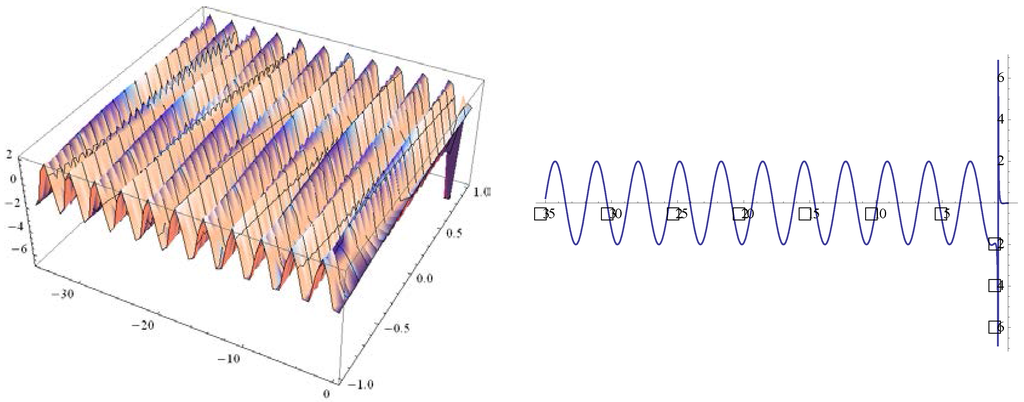
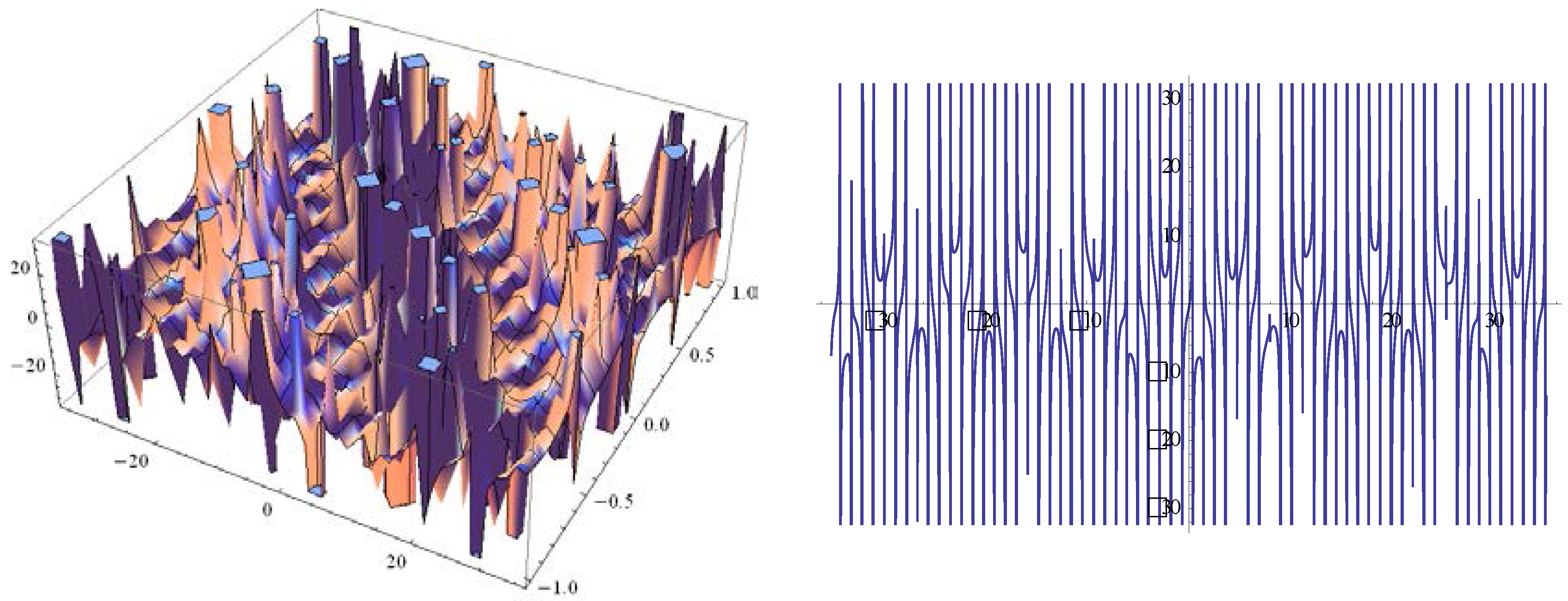
Figure 1.
Graph of imaginary values of in Equation (34) is indicated at and the second graph shows imaginary values of in Equation (34) for

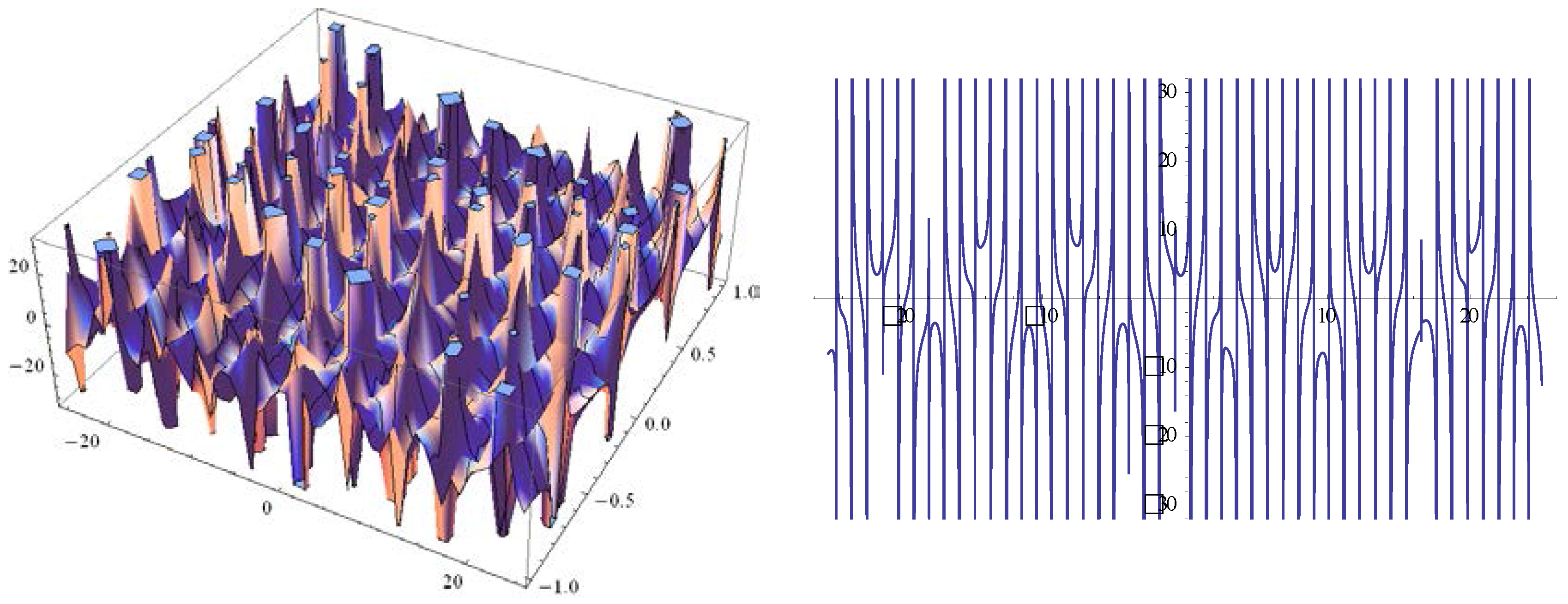
Figure 2.
Graph of real values of in Equation (34) is denoted at and the second graph remarks on real values of in Equation (34) for
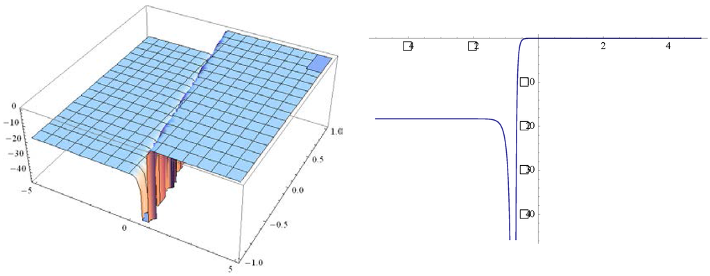
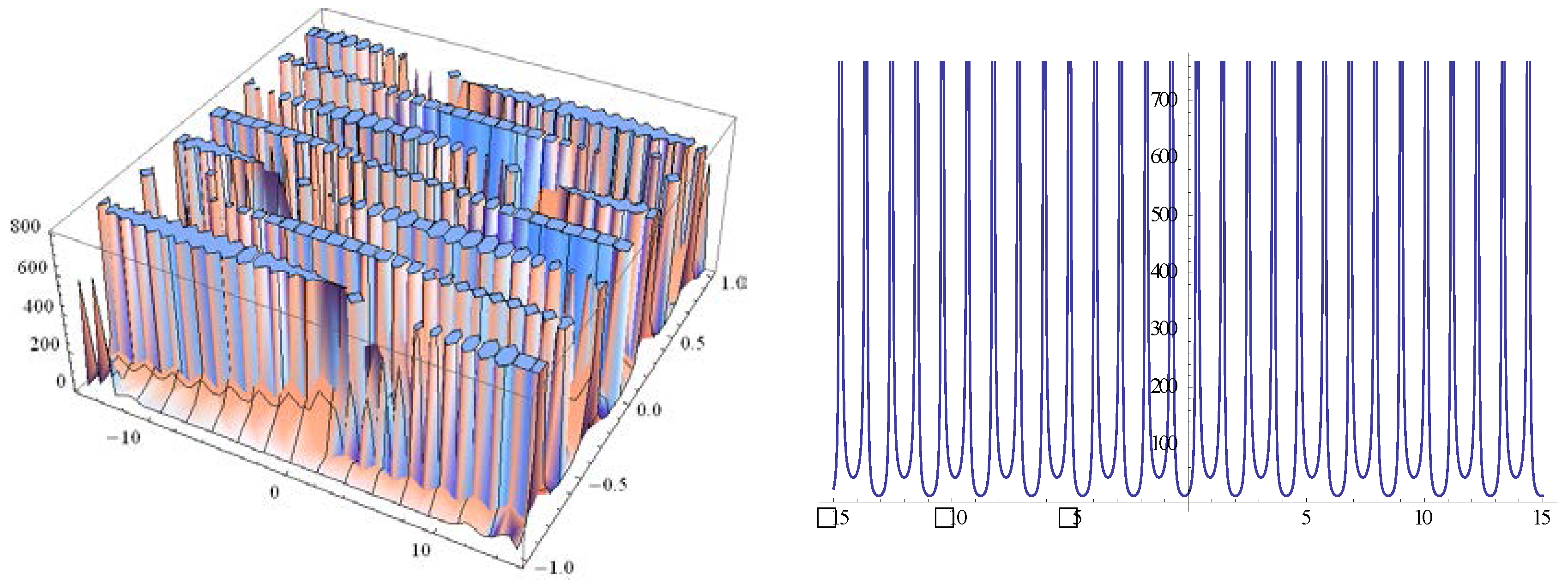
Figure 3.
Graph of in Equation (34) is drawn at and the second graph shows in Equation (34) for

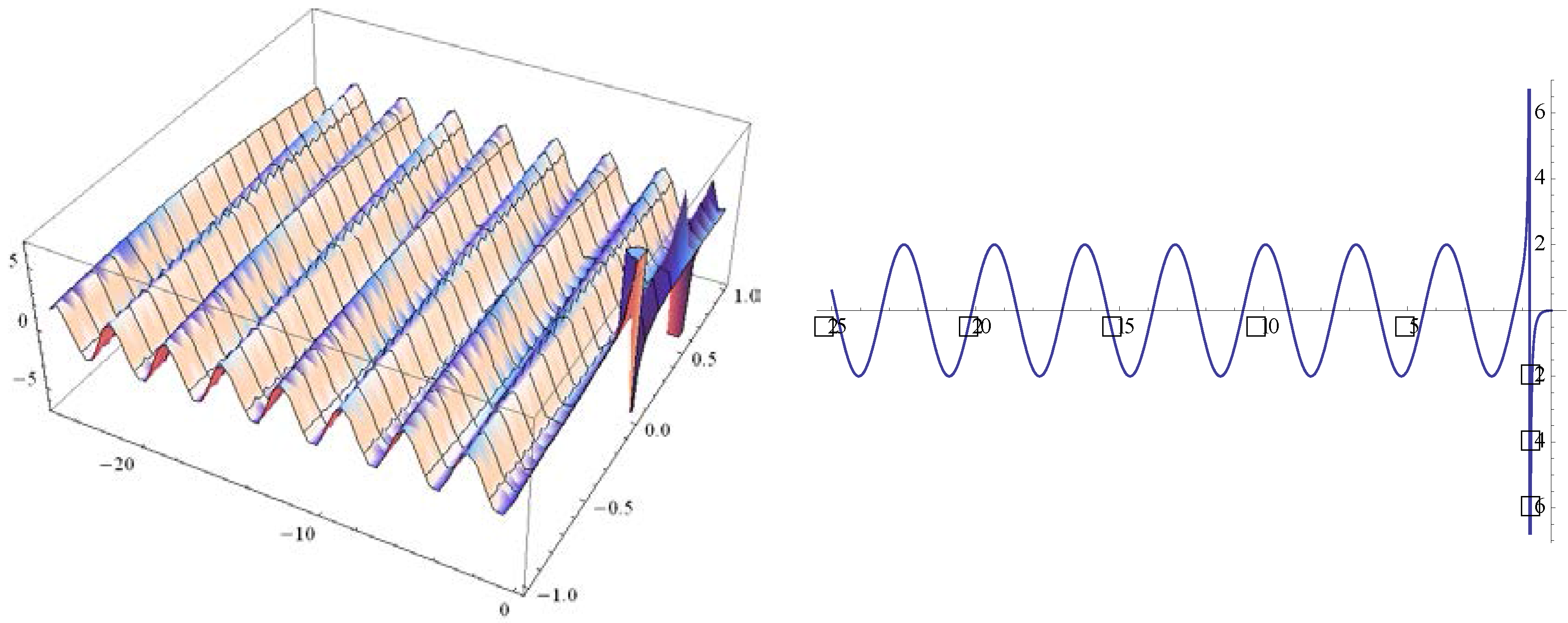
Figure 4.
Graph of imaginary values of in Equation (36) is indicated at and the second graph illustrates imaginary values of in Equation (36) for

Figure 5.
Graph of real values of in Equation (36) is denoted at , and the second graph remarks on real values of in Equation (36) for

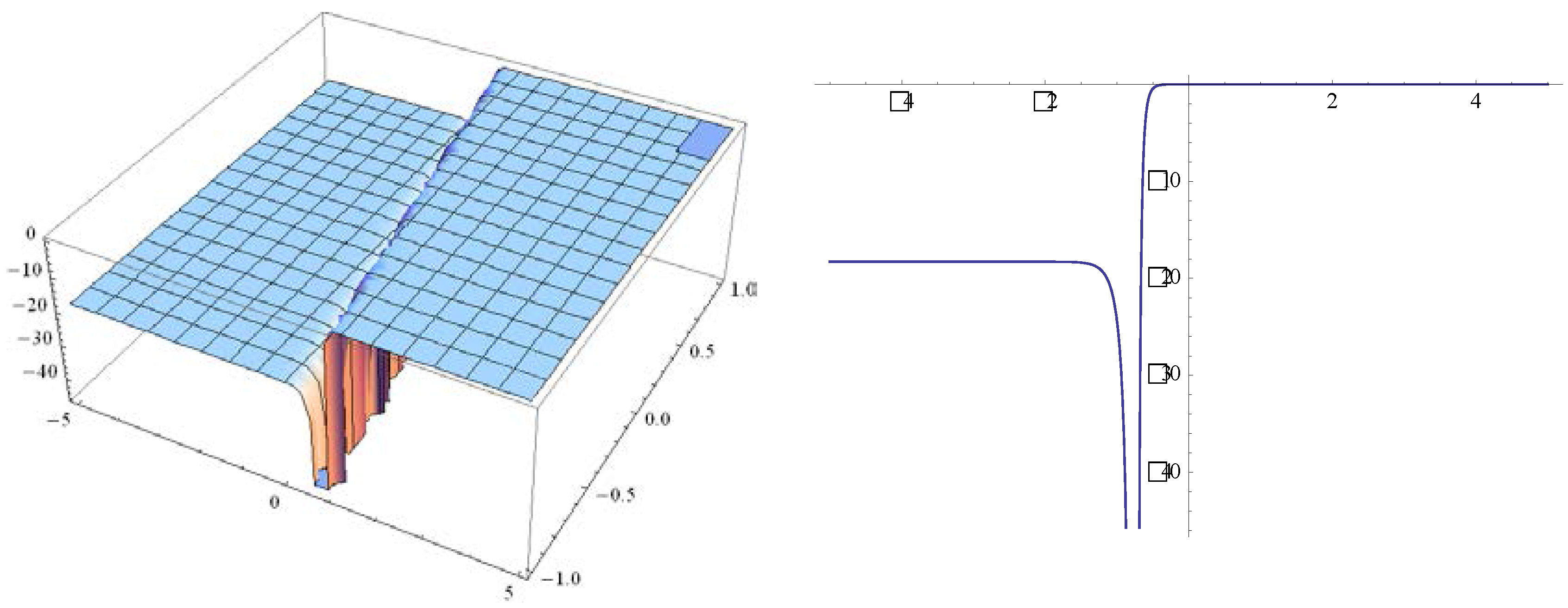
Figure 6.
Graph of in Equation (36) is drawn at , and the second graph illustrates in Equation (36) for
Acknowledgments
The authors would like to thank the reviewers for their valuable comments and suggestions to improve the present work.
Author Contributions
All authors have equally contributed to this paper. They have read and approved the final version of the manuscript.
Conflicts of Interest
The authors declare no conflict of interest.
References
- Degtyarev, L.M.; Nakhan’kov, V.G.; Rudakov, L.I. Dynamics of the formation and interaction of Langmuir solitons and strong turbulence. Zhurnal Eksp. Teor. Fiz. 1974, 67, 533–542. [Google Scholar]
- Degtyarev, L.M.; Zakharov, V.E.; Sagdeev, R.Z.; Solov’ev, G.I.; Shapiro, V.D.; Shevchenko, I.V. Langmuir collapse under pumping and wave energy dissipation. Zhurnal Eksp. Teor. Fiz. 1983, 85, 1221–1231. [Google Scholar]
- Anisimov, S.I.; Berezovskii, M.A.; Ivanov, M.F.; Petrov, I.V.; Rubenchick, A.M.; Zakharov, V.E. Computer simulation of the Langmuir collapse. Phys. Lett. A 1982, 92, 32–34. [Google Scholar] [CrossRef]
- Anisimov, S.I.; Berezovskii, M.A.; Zakharov, V.E.; Petrov, I.V.; Rubenchik, A.M. Numerical simulation of a Langmuir collapse. Zhurnal Eksp. Teor. Fiz. 1983, 84, 2046–2054. [Google Scholar]
- D’yachenko, A.I.; Zakharov, V.E.; Rubenchik, A.M.; Sagdeev, R.Z.; Shvets, V.F. Numerical simulation of two-dimensional Langmuir collapse. Zhurnal Eksp. Teor. Fiz. 1988, 94, 144–155. [Google Scholar]
- Zakharov, V.E.; Pushkarev, A.N.; Rubenchik, A.M.; Sagdeev, R.Z.; Shvets, V.F. Numerical simulation of three-dimensional Langmuir collapse in plasma. Zhurnal Eksp. Teor. Fiz. 1988, 47, 287–290. [Google Scholar]
- Benilov, E.S. Stability of plasma solitons. Zhurnal Eksp. Theor. Fiz. 1985, 88, 120–128. [Google Scholar]
- Zakharov, V.E.; Pushkarev, A.N.; Sagdeev, R.Z.; Soloviev, S.I.; Shapiro, V.D.; Shvets, V.F.; Shevchenko, V.I. “Throughout” modelling of the one-dimensional Langmuir turbulence. Sov. Phys. Dokl. 1989, 34, 248–251. [Google Scholar]
- Dyachenko, A.I.; Pushkarev, A.N.; Rubenchik, A.M.; Sagdeev, R.Z.; Shvets, V.F.; Zakharov, V.E. Computer simulation of Langmuir collapse. Phys. D 1991, 52, 78–102. [Google Scholar] [CrossRef]
- Rubenchik, A.M.; Zakharov, V.E. Strong Langmuir Turbulence in Laser Plasma; Handbook of Plasma Physics; Elsevier Science Publishers: Amsterdam, The Netherlands, 1991; Volume 3, pp. 335–360. [Google Scholar]
- Musher, S.L.; Rubenchik, A.M.; Zakharov, V.E. Weak Langmuir turbulence. Phys. Rep. 1995, 252, 178–274. [Google Scholar] [CrossRef]
- Robinson, P.A.; Willes, A.J.; Cairns, I.H. Dynamics of Langmuir and ion-sound waves in type III solar radio sources. Astrophys. J. 1993, 408, 720–734. [Google Scholar] [CrossRef]
- Chen, Y.-H.; Lu, W.; Wang, W.-H. The Nonlinear Langmuir Waves in a Multi-ion-Component Plasma. Commun. Theor. Phys. 2001, 35, 223–228. [Google Scholar]
- Soucek, J.; Krasnoselskikh, V.; de Wit, T.D.; Pickett, J.; Kletzing, C. Nonlinear decay of foreshock Langmuir waves in the presence of plasma inhomogeneities: Theory and Cluster observations. J. Geophys. Res. 2005, 110, 1–10. [Google Scholar] [CrossRef]
- Dodin, I.Y.; Geyko, V.I.; Fisch, N.J. Langmuir wave linear evolution in inhomogeneous nonstationary anisotropic plasma. Phys. Plasmas 2009, 16, 1–9. [Google Scholar] [CrossRef]
- Zaslavsky, A.; Volokitin, A.S.; Krasnoselskikh, V.V.; Maksimovic, M.; Bale, S.D. Spatial localization of Langmuir waves generated from an electron beam propagating in an inhomogeneous plasma: Applications to the solar wind. J. Geophys. Res. 2010, 115, 1–11. [Google Scholar] [CrossRef]
- Ratcliffe, H.; Brady, C.S.; Rozenan, M.B.C.; Nakariakov, V.M. A comparison of weak-turbulence and particle-in-cell simulations of weak electron-beam plasma interaction. AIP Phys. Plasmas 2014, 21, 1–9. [Google Scholar] [CrossRef]
- Ajima, N.Y.; Wa, M.O. Formation and Interaction of Sonic-Langmuir Solitons. Prog. Theor. Phys. 1976, 56, 1719–1739. [Google Scholar] [CrossRef]
- Zakharov, V.E. Collapse of Langmuir Waves. Zhurnal Eksp. Teor. Fiz. 1972, 62, 1745–1759. [Google Scholar]
- Zhen, H.-L.; Tian, B.; Wang, Y.-F.; Liu, D.-Y. Soliton solutions and chaotic motions of the Zakharov equations for the Langmuir wave in the plasma. AIP Phys. Plasmas 2015, 22. [Google Scholar] [CrossRef]
- Dubinov, A.E.; Kitayev, I.N. New solutions of the Zakharov’s equation system for quantum plasmas in form of nonlinear bursts lattice. AIP Phys. Plasmas 2014, 21. [Google Scholar] [CrossRef]
- Khan, Y.; Faraz, N.; Yildirim, A. New soliton solutions of the generalized Zakharov equations using He’s variational approach. Appl. Math. Lett. 2011, 24, 965–968. [Google Scholar] [CrossRef]
- Yang, X.-L.; Tang, J.-S. Explicit exact solutions for the generalized Zakharov equations with nonlinear terms of any order. Comput. Math. Appl. 2009, 57, 1622–1629. [Google Scholar]
- Javidi, M.; Golbabai, A. Exact and numerical solitary wave solutions of generalized Zakharov equation by the variational iteration method. Chaos Solitons Fractals 2008, 36, 309–313. [Google Scholar] [CrossRef]
- Wang, Y.-Y.; Dai, C.-Q.; Wu, L.; Zhang, J.-F. Exact and numerical solitary wave solutions of generalized Zakharov equation by the Adomian decomposition method. Chaos Solitons Fractals 2007, 32, 1208–1214. [Google Scholar] [CrossRef]
- De Oliveira, G.I.; Rizzato, F.B. Scaling laws for breathing frequencies of solitary modes in the Zakharov equations. Phys. Rev. E 2001, 65. [Google Scholar] [CrossRef] [PubMed]
- Bulut, H.; Pandir, Y.; Demiray, S.T. Exact Solution of Nonlinear Schrödinger’s Equation with Dual Power-Law Nonlinearity by Extended Trial Equation Method. Waves Random Complex Media 2014, 24, 439–451. [Google Scholar] [CrossRef]
- Demiray, S.T.; Pandir, Y.; Bulut, H. New Soliton Solutions for Sasa-Satsuma Equation. Waves Random Complex Media 2015, 25, 417–428. [Google Scholar] [CrossRef]
- Demiray, S.T.; Pandir, Y.; Bulut, H. New Solitary Wave Solutions of Maccari System. Ocean Eng. 2015, 103, 153–159. [Google Scholar] [CrossRef]
- Demiray, S.T.; Bulut, H. New Exact Solutions of the New Hamiltonian Amplitude Equation and Fokas Lenells Equation. Entropy 2015, 17, 6025–6043. [Google Scholar] [CrossRef]
- Demiray, S.T.; Bulut, H. Some Exact Solutions of Generalized Zakharov System. Waves Random Complex Media 2015, 25, 75–90. [Google Scholar] [CrossRef]
- Demiray, S.T.; Pandir, Y.; Bulut, H. All Exact Travelling Wave Solutions of Hirota Equation and Hirota-Maccari System. Optik 2016, 127, 1848–1859. [Google Scholar] [CrossRef]
- Pandir, Y.; Gurefe, Y.; Kadak, U.; Misirli, E. Classification of exact solutions for some nonlinear partial differential equations with generalized evolution. Abstr. Appl. Anal. 2012, 2012. [Google Scholar] [CrossRef]

© 2016 by the authors; licensee MDPI, Basel, Switzerland. This article is an open access article distributed under the terms and conditions of the Creative Commons by Attribution (CC-BY) license (http://creativecommons.org/licenses/by/4.0/).