Research on Object Detection Model Based on Feature Network Optimization

Abstract

As the object detection dataset scale is smaller than the image recognition dataset ImageNet scale, transfer learning has become a basic training method for deep learning object detection models, which pre-trains the backbone network of the object detection model on an ImageNet dataset to extract features for detection tasks. However, the classification task of detection focuses on the salient region features of an object, while the location task of detection focuses on the edge features, so there is a certain deviation between the features extracted by a pretrained backbone network and those needed by a localization task. To solve this problem, a decoupled self-attention (DSA) module is proposed for one-stage object-detection models in this paper. A DSA includes two decoupled self-attention branches, so it can extract appropriate features for different tasks. It is located between the Feature Pyramid Networks (FPN) and head networks of subtasks, and used to independently extract global features for different tasks based on FPN-fused features. Although the DSA network module is simple, it can effectively improve the performance of object detection, and can easily be embedded in many detection models. Our experiments are based on the representative one-stage detection model RetinaNet. In the Common Objects in Context (COCO) dataset, when ResNet50 and ResNet101 are used as backbone networks, the detection performances can be increased by 0.4 and 0.5% AP, respectively. When the DSA module and object confidence task are both applied in RetinaNet, the detection performances based on ResNet50 and ResNet101 can be increased by 1.0 and 1.4% AP, respectively. The experiment results show the effectiveness of the DSA module.

1. Introduction

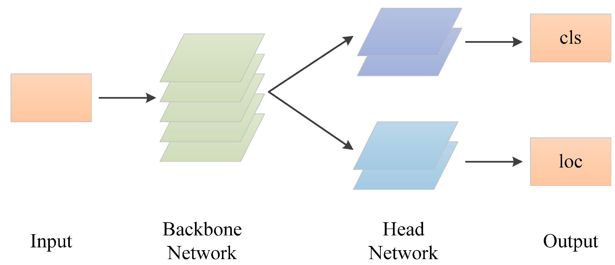
The ImageNet [1] dataset is a large-scale image-classification dataset built by Professor Li Fei-Fei, which contains tens of millions of images and tens of thousands of categories of objects. The dataset greatly promotes the development of image recognition. It can also improve other more complex Computer Vision (CV) tasks by transfer learning, such as object detection and instance segmentation. An object detection task contains two subtasks, classification and localization, and they focus on the different spatial features of objects; for example, a classification task focuses on salient area features and a localization task focuses on edge features [2]. Therefore, the features extracted by the pretrained backbone network are not entirely suitable for localization tasks. To learn the suitable features for both tasks, some detectors are trained on object detection datasets from scratch [3,4,5]. Although their performances are close to those of detectors using the transfer learning strategy, they need a longer training time and abundant expert experience. Therefore, most object detectors still prefer transfer learning in training at present. In order to use transfer learning in object detection, we propose a method to extract features from pretrained features by introducing a self-attention mechanism, which can automatically extract relevant features for a specific task.

The attention mechanism comes from brain imaging mechanism research. When people observe a scene, they generally pay more attention to salient objects and less attention to backgrounds. Then, this is introduced into deep-learning networks to distinguish the importance of different features in a task. Generally, weight is used to represent the importance of features: the larger the weight, the more important the feature. In 2014, Bahdanau et al. first introduced attention to an NLP machine translation task [6]. The translation model included two processes: encoder and decoder. They applied the attention mechanism to the decoder stage to solve the problem of long-distance dependences in machine translation. “Attention is all you need” [7], published by the Google team in 2017, proposed a new machine translation model, Transformer, which only uses the attention mechanism, instead of Convolutional Neural Networks (CNN) or Recurrent Neural Networks (RNN), to extract features in encoder stages, which greatly improves the performance of a machine translation task. Then, Google proposed a pretrained model, Bert [8], in the Natural Language Processing (NLP) field, based on Transformer. Bert not only reduces the training time of most NLP tasks, such as named entity recognition, machine translation and reading comprehension, it also greatly improves the performances of these tasks. The most important contribution of Transformer is that it proposes the feature extraction method using a self-attention mechanism, which is used to learn the relationship between self(input) and self(input), called self-attention. Self-attention can capture the internal correlation of all features, so each input feature can contain all the input information. Recently, some research works have introduced the attention mechanism to the CV field. Squeeze-and-Excitation Networks (SENet) [9] achieved the best results in the 2017 ImageNet competition, and its most important innovation is that it designs an attention module in the channel domain. The module can learn the weight of each channel, which represents the importance of each channel to the output, and is used to recalibrate features for a task, which leads the output to pay more attention to important channel features and suppress invalid channel features. Although the structure of channel attention of SENet is simple, the idea promotes the development of an attention mechanism in the CV field. Convolutional Block Attention Module (CBAM) [10] further explored the application scope of an attention mechanism and proposed a combination of the channel attention module and spatial attention module. The channel attention module was used to learn the channel features that needed to be focused on, and the spatial attention module was used to learn the spatial location features that needed to be paid attention. The non-local Net [11] used only the self-attention mechanism to learn features, which is very similar to Transformer’s method. It enables each feature to learn global context information, solving the problem of a small receptive field for the features extracted by convolution network. This work can achieve excellent performances in object detection and video-tracking tasks, although there is too much computation in the model. Dual Attention Network (DANet) [12] applied the attention mechanism to image segmentation tasks. The smaller receptive field of convolution features resulted in the pixel from the same object having different classes, which restricts the segmentation performance. It used spatial and channel self-attention modules to extract features containing global spatial and channel information, which effectively improved segmentation performance.

From the above, we can see that the attention mechanism was applied to many image tasks, but there are few works on object detection. Object detection consists of two subtasks focusing on the different spatial features of objects, and the attention mechanism can learn the importance of different spatial features. Therefore, introducing attention to object detection is a natural step. Besides this, self-attention is generally used in the feature-extraction stage. Therefore, we propose an object detection model, DSANet, based on the self-attention mechanism, and uses the spatial domain self-attention module decoupled self-attention (DSA) to extract suitable features for specific tasks. DSA also supplies two different feature-extracted branches for classification and localization tasks, which is why it is called decoupled self-attention. In summary, the main contributions of this paper are described as follows:

(1)

To make full use of pretrained backbone network in one-stage object detection, we propose a decoupled module to extract suitable features for specific tasks;

(2)

As the two subtasks of object detection focus on the different spatial features of objects, the decoupled module uses the spatial self-attention mechanism to learn more suitable features for different tasks; the module is called DSA in this paper;

(3)

In order to validate the DSA module, we propose an object-detection model DSANet based on RetinaNet. All experiments are built on the COCO dataset; the DSA module can improve 0.4 and 0.5% AP with ResNet-50 and ResNet-101 [13] backbone networks, respectively. We further build an object detection model, DSANet-Conf, which applies both the DSA module and object confidence subtask [14] to RetinaNet. It can gain 36.3 and 38.4% AP with ResNet-50 and ResNet-101 backbone networks, respectively. The experiment results show that the DSA module can improve the one-stage object detection model.

2. Related Work

Many studies on the extraction of suitable features for two tasks in an object-detection model have been published. The object-detection model has four parts: input, backbone network, head network and output, as shown in Figure 1. The existing works are mainly divided into three categories: (1) improvement in backbone network; (2) training from scratch; (3) improvement in the head networks of subtasks.

(1)

Improvement in backbone network. At present, the most commonly used backbone network for object detection is FPN [15], which uses fused features to improve classification and localization tasks. Path Aggregation Network (PANet) [16] thought that the location information of top-level features in FPN was greatly weakened by dozens or hundreds of convolution layers, so it proposed a bottom-up pathway for FPN. In order to improve the detection performance without significantly increasing model parameters and computation, a multiscale object detection method, Scale-Transferrable Object Detection (STDN) [17], based on DenseNet [18], was proposed. M2Det [19] gathered the advantages of FPN and PANet, so that it is more suitable for object detection. Gated Feedback Refinement Network (G-FRNet) [20] proposed a gating unit to filter the fuzzy semantics from low-level features through high-level features to improve the class-distinguishing ability of low-level features. NAS-FPN [21] was automatically created by NAS, and can balance model accuracy and efficiency. EfficientDet [22] is an efficient and accurate object detection model and can gain the same excellent performance as PANet, with less computation. Differing from the above, RFBNet [23] improves the semantic information of low-level features by introducing dilated convolution;

(2)

Training from scratch. “Rethinking ImageNet Pre-training” [3], published by Kaiming He et al., proved that object detection without a pretrained backbone network can still converge after more training iterations. However, DSOD [5] thought that it was unstable to train a detection model from scratch. Then, ScratchDet [4] delved into this problem and fought that the main reason for this was that BN was not used in the model. When BN was added to the model, it could train stably, and the performance was better than that of a pretrained model. DetNet [24] was a specific backbone network designed for object detection tasks. It used dilated convolution to increase the receptive field of features without reducing the scale of the feature map. This could not only retain the location details of objects, but also improved the context information of features;

(3)

Improvement in head networks. RetinaNet [25] first proposed the head network with four convolution layers for each subtask, so it could extract specific features for each task. The detection performance was reduced by about 10% AP without head networks, which showed the importance of extracting independent features for each subtask. Double-head Region Convolutional Neural Networks (RCNN) [26] used fc and convolution networks after Region of Interest (RoI) [27] pooling features for classification and localization tasks, respectively. Inspired by Double Head RCNN, the Sense Time team delved into the differences in the features used for two subtasks [2] and proposed a Task-aware Spatial Disentanglement (TSD) module, including different styles of deformable convolution to extract suitable features for different tasks from ROI pooling features.

According to the above analysis, the “improvement in backbone network” method needs more expert experience for uses designing network architecture. Although it can improve the feature presentation, more time and computation is needed for it to find the optimal architecture from infinite solution space. The “training from scratch” method can learn suitable features for different tasks, but it needs to configure parameters carefully and requires more training time. The “improvement in head networks” method does not modify the backbone network; it only adds an independent head network for each task. Therefore, we can still use a pretrained network, which can extract individual features for different tasks and extract appropriate features with less training time. We improve the performance of detection model based on the “improvement in head networks” method. In order to reduce human experience in head network design, the head network in this paper uses a self-attention mechanism to automatically extract features for each task.

3. Methods

In this section, we will introduce DSANet in more detail. Firstly, we show the network architecture of DSANet, which adds a DSA module to RetinaNet. Then, we introduce the attention mechanism used in DSA and analyze the differences between different attention operations. Finally, we introduce the training and inference processes of DSANet.

3.1. Architecture of Retinanet-Conf Detector

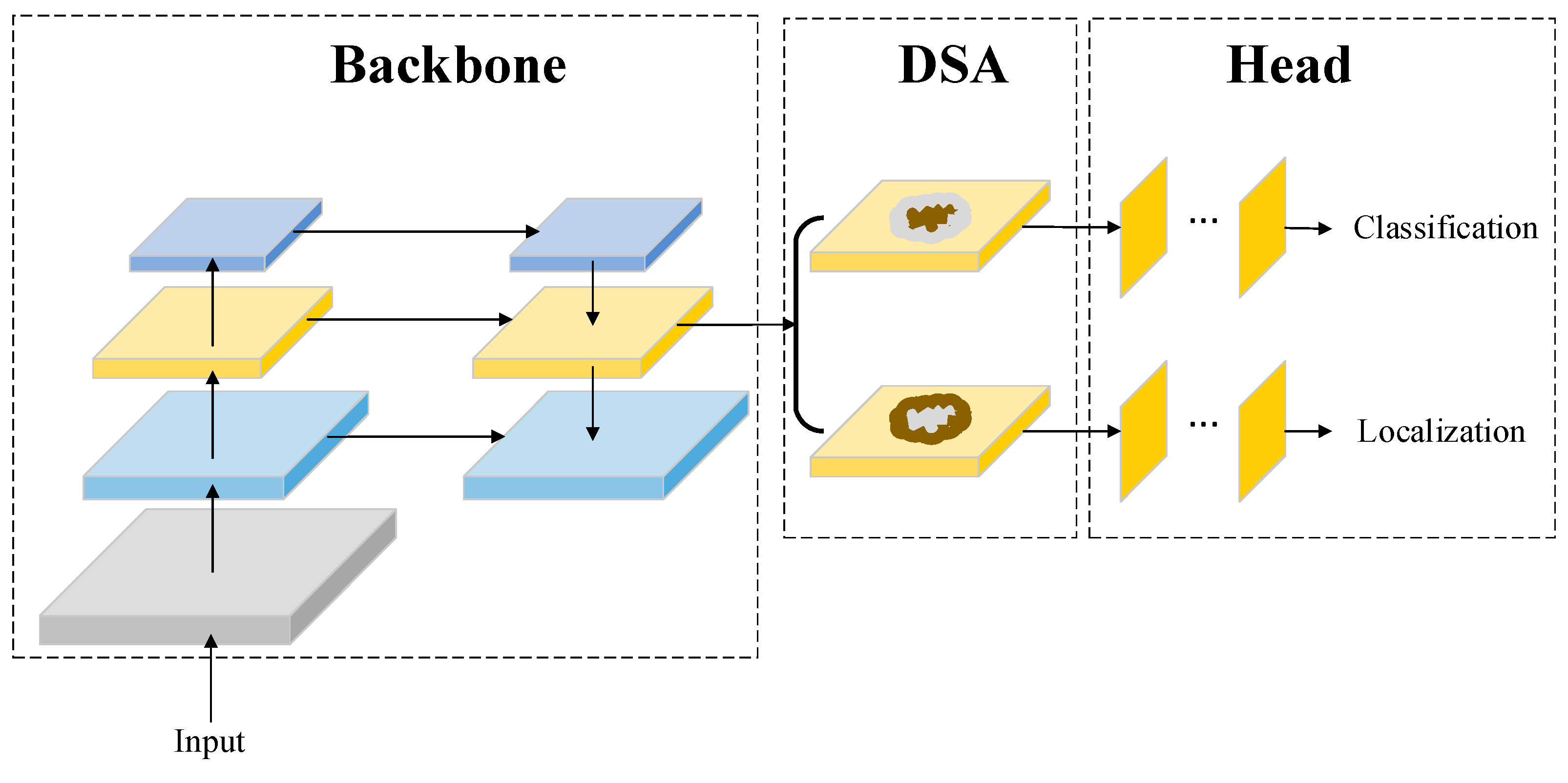
A DSA module consists of two branches, using the self-attention mechanism to extract features for classification and localization tasks. As shown in Figure 2, the top branch of DSA extracts the salient region features of objects for classification tasks, and the down branch extracts the edge features of objects for localization tasks. Existing object detection models generally use FPN as a backbone network, then use different scale features to detect different scale objects. DSANet adds a DSA module after each FPN fusion feature to extract notable features of different scale objects. DSA only uses the self-attention mechanism in the spatial domain of convolution features, because classification tasks and location tasks focus on the different spatial features of objects.

DSA can be calculated by Equation (1):

$$Feature\text{\_}att=Attention(f(Feature\text{\_}input))$$

(1)

In Equation (1), $Feature\text{\_}input$ is the input of DSA, $Feature\text{\_}att$ is the output of attention operation, $f$ represents preprocess function on input, and generally includes max-pooling, average-pooling and 1 $\times$ 1 convolution operations. $Attention$ represents the attention operation, and can use the learned method or vector similarity calculation method to define the weights of features. In this paper, $Attention$ is self-attention, so $f$ will use three 1*1 convolution networks to generate three features representing input, and the similarity method is used to calculate the weights of spatial features through the correlation between them.

Then, we can use Equation (2) to calculate the output of the DSA module:

$$Feature\text{\_}out=Feature\text{\_}input+\gamma *Feature\text{\_}att$$

(2)

In Equation (2), $Feature\text{\_}out$ represents the output of the DSA module. From the equation, we can see that the DSA module uses the same calculation method as the residual module of ResNet, and its input is directly connected to its output. The attention output features work as a branch of DSA output, and $\gamma$ is a learned parameter, which is used to balance the importance of initial input and attention output. Therefore, a DSA module with a residual design can focus on important features without increasing the model’s training difficulties.

As self-attention is used in the DSA module, each feature of its output and attention output contains global spatial context information. The DSA module is located before the head network, which ensures that each head network feature will contain global spatial context information that is critical to classification and localization tasks, so that the DSA module can improve object detection performance, especially for small objects.

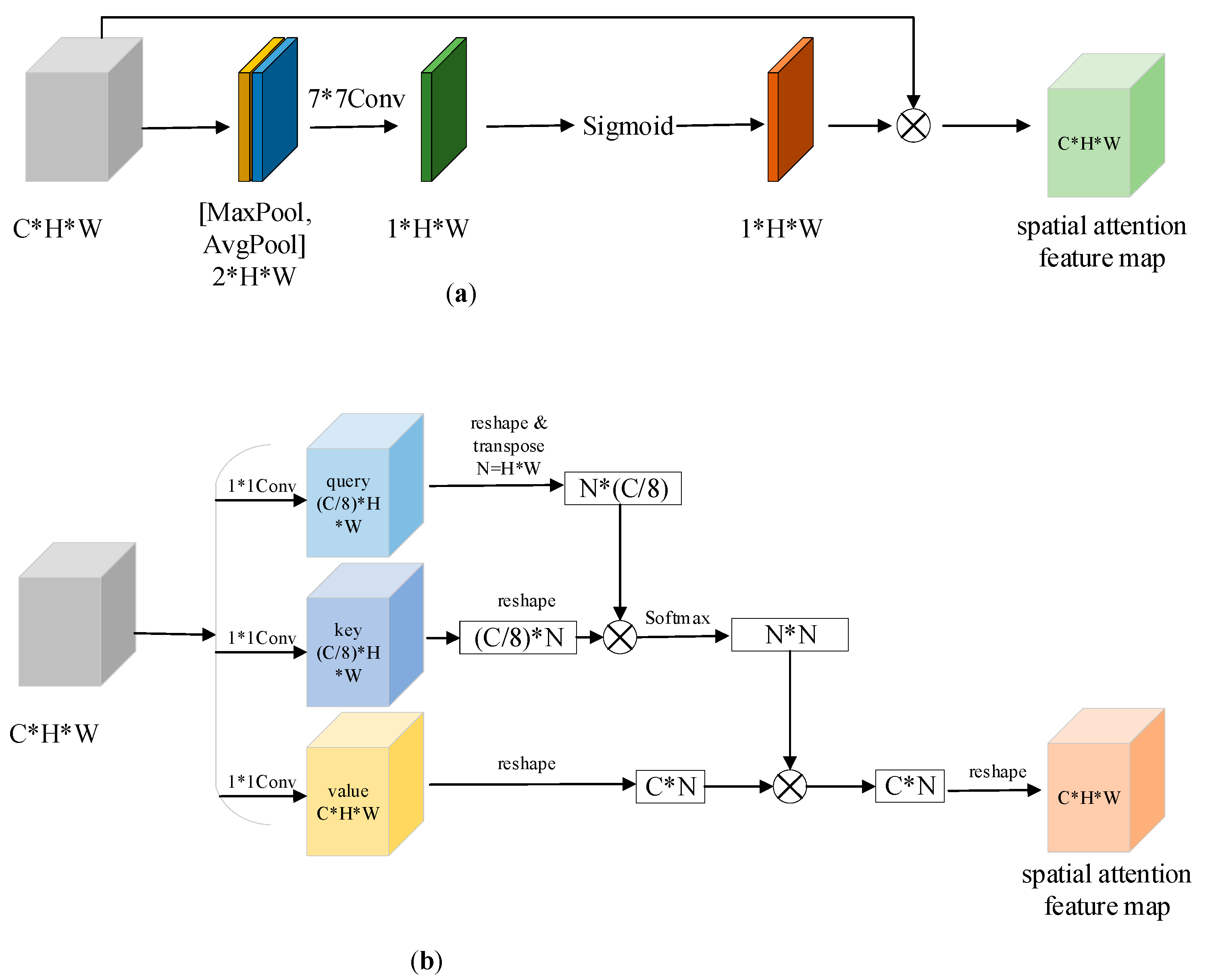
From the above description, we know that DSA uses spatial attention to extract features. There are two spatial attention methods in computer vision: (1) using a convolution network to learn the attention weight for each objects’ spatial position, and the spatial attention feature map is the product of attention weight and input features; (2) using the self-attention mechanism to calculate the weights between two spatial position features, and each spatial position output feature is the weighted sum of the weights and values of other spatial position features. Figure 3 shows the two spatial attention feature maps’ generated methods.

The spatial attention method in Figure 3a is inspired by the channel attention of SENet. The channel attention of SENet first calculates the mean of each channel feature, and the mean value works as the input of a two-layer, fully connected(fc) network, and the output of the fc network is the weight of each channel. Figure 3a calculates the maximum and mean of each spatial position feature; then, a 7 $\times$ 7 convolution is used to reduce feature dimensions from 2D to 1D. The 1D features will be used as the sigmoid function input, the output is the weight of each spatial position feature, and all channels share the weight of the same spatial position. The spatial attention features can be calculated by Equations (3) and (4).

$$\begin{array}{cc}\hfill {\mathrm{M}}_S(F)& =\sigma (Con{v}^{7*7}([MaxPool(F),AvgPool(F)]))\hfill \\ \hfill & =\sigma (Con{v}^{7*7}([F_{\max }^S,F_{avg}^S]))\hfill \end{array}$$

(3)

$$F_{spatial\text{\_}att}=F\otimes {\mathrm{M}}_S(F)$$

(4)

In Equation (3), ${\mathrm{M}}_S(F)$ represents the weight results of all spatial positions of objects, $F$ is the input of attention module. $MaxPool$ and $AvgPool$ represents max pooling and average pooling operation, $F_{\max }^S$ and $F_{avg}^S$ are the output features after different pooling operations. Equation (4) shows the calculation of spatial attention features through the input and weights of spatial position.

Figure 3b shows the spatial attention features calculation process based on self-attention, which is introduced from the machine translation model Transformer. Vaswani et al. summarized the attention function [7], which is shown as Equation (5):

$$Attention(Q,K,V)=soft\max (\frac{Q{K}^T}{\sqrt{d_k}})V$$

(5)

In Function (5), $Q$, $K$, $V$ represent Query, Key and Value. Query is a query matrix, used to represent the affected samples. If the dimension of query matrix is $N*d_k$, and $N$ represents the number of affected samples, $d_k$ represents the dimension of features in each samples. Key and Value are the different representations of impact samples, and [Key, Value] can be seen as the key/value pair of impact samples; Key is used to identify which sample, while Value represents the value of the sample, so they are a one-to-one match. If their dimensions $M*d_k$, $M$ represents the number of impact samples and $d_k$ represents the dimension of features in an impact sample. We can find that the feature dimensions of the impact sample and affected samples are same. $Q{K}^T$ is the matrix product of matrix $Q$ and $K^T$, which shows the similarity results of affected samples and impact samples. $soft\max (\frac{Q{K}^T}{\sqrt{d_k}})$ can be used to calculate the weights of all impact samples and each affected sample, so the product of this and the matrix Value is the spatial attention features. Equation (5) shows the common attention calculation function; the matrix Query, Key and Value are all representations of impact samples when they represent self-attention. As the source of the Query matrix is same as that of Key and Value, this attention is called self-attention.

From Figure 4a, we can see that each spatial feature of output is only related to one spatial feature of input, so the output features do not contain the global spatial context information. However, from Figure 4b we can see that each spatial feature of output is related to every spatial feature of input, so every feature of output contains global spatial context information. In addition, each spatial feature of output owns the unique weights between other the spatial features with this feature, so the focused area of each spatial feature in the output is different. In summary, the attention in Figure 4a is essentially different from the attention in Figure 4b. Figure 4a uses a convolution network to learn the weights of each spatial feature from channel global information. The weight represents the importance of each spatial feature in the next layer of features. Therefore, the receptive field of the output feature is same as that of an input feature, which shows the semantic information of feature is not improved with the deep increase in network. Besides this, the filter size convolution size is 7*7, so it will provide a large number of parameters and large amount of computation, which will increase the model’s training difficulty. However, Figure 4b, using self-attention, not only uses global receptive field information to improve feature representation, but also brings many additional model parameters. However, we should note that self-attention has a higher computation cost, because the computation of $soft\max (\frac{Q{K}^T}{\sqrt{d_k}})V$ is $d_k*N*N*N$, $N$ is equal to $H*W$, and $d_k$ is the number of channels. When using the self-attention mechanism on the feature map with a higher resolution, the huge amount of computation will result in a lack of Graphic Processing Unit (GPU) memory. Therefore, it is necessary to carefully select the feature map, adding the DSA module when computation resources are insufficient. However, from the characteristics of CNN, we know that the receptive field of feature map with higher resolution is generally smaller, and represents less context information, so these feature maps need the DSA module more, as well as more computation. Therefore, it is worth researching how to balance the context information and computation of a high-resolution feature map with DSA module.

3.2. Training and Inference

DSANet adds an DSA module to the middle of RetinaNet. The model training process mainly updates network parameters according to the loss function. As the DSANet modifies model task, it has same loss function as RetinaNet. Therefore, the loss function of DSANet also includes two parts: classification loss function and localization loss function. We will not repeat these here again. As the DSA module is added after the FPN network, we can still use pretrained ResNet parameters. Therefore, the added DSA module will not slow the parameter-training efficiency of FPN and head network. Therefore, the initialization and training settings of these parameters can be consistent with RetinaNet. From Equation (2), we can see that a new parameter $\gamma$ is added to measure the percentage of the attention feature map in the DSA output. To train this parameter, we initialize this to 0 and update it using the same update strategy as other network parameters in the training process. The inference process of the model mainly focuses on the selection of box prediction results, such NMS. Similarly, the DSA module will not affect the selection process of detection results, so the inference process is also consistent with RetinaNet.

4. Experiments

In order to validate DSANet, we used the large-scale benchmark-object-detection dataset MS coco 2017 in experiments. This included Train2017, Val2017 and Test2017. Train2017 includes 118,287 images, Val2017 includes 5000 images, and Test2017 includes 40,670 images. Test2017 is generally used in some competitions, so this paper only used Train2017 and Val2017 in the experiments. Train2017 is used for training and Val2017 is used for validation, and all APs and Recalls indexes, defined by the coco dataset, are used for evaluation. As DSANet is based on RetinaNet, and MMDetection [28] is an excellent open CV task sources platform by Shang Tang, all experiments in this paper were performed on the RetinaNet source code in MMDetection. The experiment environment included 16 G memory, 8-core CPU and a Tesla V100 GPU with 32 G memory. The input size of the model was [1000,600], the batch size was 16 and the total training epoch was 12. The optimizer was Stochastic Gradient Descent (SGD), with an initial learning rate of 0.01. The learning rate decayed 0.1 times in epoch [9,12].

From

Table 1. Comparison of DSA modules using different attention methods. DSANet_a uses the attention method shown in Figure 3a, while DSANet_b uses the attention method shown in Figure 3b; “3-7” or “4-7” shows that we add a DSA module in FPN conv3-7 or conv4-7 fusion features. As the computation of self-attention is too large, it is out of GPU memory when using self-attention in conv3 feature map with higher resolution. Hence, DSANet only adds self-attention DSA module in conv4-7 FPN fusion features, and other experiments abide by the same agreement.

Model_Name	AP	AP50	AP75	APS	APM	APL	AR	ARS	ARM	ARL
RetinaNet	0.353	0.543	0.375	0.184	0.394	0.480	0.522	0.308	0.573	0.694
DSANet_a(3-7)	0.356	0.545	0.380	0.184	0.393	0.487	0.525	0.306	0.575	0.701
DSANet_b(4-7)	0.357	0.548	0.379	0.185	0.399	0.483	0.524	0.308	0.575	0.693

, we can see that DSANet_a and DSANet_b both achieved a better detection performance than RetinaNet, which showed that the DSA module can improve object detection tasks with either attention method. Although DSANet_b did not add DSA to the conv3 feature map, DSANet_b still performed better than DSANet_a, which shows that the features extracted by self-attention have better presentation, as they contain global context information. Compared with DSANet_a, the AP₅₀ and AP_M of DSANet_b were improved by 0.3 and 0.6%AP, but AP_L and AR_L were reduced by 0.4 and 0.8%AP, and other indexes were nearly the same in the two models. The improvement in AP₅₀ shows that DSANet_b can improve the detection performance of hard examples. Although the DSA module was not added to the conv3 feature map, which was used to detect small objects, the values of AP_S, AP_M, AR_S and AR_M were improved, while AP_L and AR_L were reduced. The reason for this phenomenon may be that there was no presentation improvement in conv3 features, which resulted in the losses of smaller objects being larger, so these losses were the main factor guiding model training; hence, the performances of smaller objects were improved while the indexes of larger objects were reduced. This is an important subject, which needs continuous study. As the resolution of the conv3 feature map was larger, the number of anchor boxes based on this resolution was higher than the sum of other all anchor boxes. DSANet_b(4-7) also had an improved performance, suggesting that the detection performance could be further improved when conv3 feature map is combined with the DSA module. However, due to the GPU computation restrictions, it would be hard to validate this conclusion. Therefore, if not otherwise specified, DSANet in later experiments all represent DSANet_b(4-7).

In order to make the features extracted by a pretrained backbone network more suitable for classification and localization tasks, RetinaNet adds head networks with two branches to refine features for different tasks. To verify whether the DSA refinement module is universal to two subtasks, we designed the experiments shown in

Table 2. Comparison of whether classification and localization tasks share a DSA module. DSANet(share) represents that the classification and localization tasks of DSANet share a DSA module, namely, DSA only has one branch. DSANet shows that DSA provides two different branches for classification and localization tasks. DSAnet(share) and DSANet all add DSA module in conv4-7 feature maps.

Model_Name	AP	AP50	AP75	APS	APM	APL	AR	ARS	ARM	ARL
RetinaNet	0.353	0.543	0.375	0.184	0.394	0.480	0.522	0.308	0.573	0.694
DSANet(share)	0.356	0.547	0.377	0.187	0.397	0.474	0.524	0.309	0.576	0.694
DSANet	0.357	0.548	0.379	0.185	0.399	0.483	0.524	0.308	0.575	0.693

. Compared with base RetinaNet, DSANet(share) and DSANet both improved the performance, while DSANet gained 0.1% AP higher than DSANet(share), which shows that the DSA module can improve feature representation. Although DSANet performed slightly better than DSANet(share) in AP index, all other indexes, except for AP_S, were improved. AP_L was also greatly increased by 0.9%, which shows that the false detection rate was reduced, especially for medium and large objects. For all recall indexes, total AR was the same, but other indexes of DSANet were slightly lower than those of DSANet(share), which shows that the missed detection rate of DSANet increased. Therefore, decoupled self-attention can extract more suitable features for different tasks from backbone network features, as well as gain higher precision, and almost all AP indexes were effectively improved. However, the missed detection rates increased in all scales objects, which may be caused by dense objects, because the detection performance of these objects was improved but they were too dense to be left in NMS. Therefore, the share of the DSA module can be regarded as a strategy to balance the false and missed detection rate requirements. If a task concerns the false detection rate, it can choose the DSANet and will require more computation, while the task concerning missed detection rates can choose DSANet(share).

In order to locate the DSA module on the right of the RetinaNet, the experiments shown in

Table 3. Comparison of different DSA module location. DSANet(before) represents the location of DSA modules between backbone and head network, and DSANet(after) represents the location of DSA modules after head network.

Model_Name	AP	AP50	AP75	APS	APM	APL	AR	ARS	ARM	ARL
RetinaNet	0.353	0.543	0.375	0.184	0.394	0.480	0.522	0.308	0.573	0.694
DSANet(after)	0.355	0.545	0.377	0.183	0.399	0.483	0.524	0.307	0.574	0.689
DSANet(before)	0.357	0.548	0.379	0.185	0.399	0.483	0.524	0.308	0.575	0.693

were designed. Therefore, to use a pretrained backbone network to train efficiently, we selected two DSA module locations, as shown in Figure 5. As shown in Table 3, DSANet(before) performed better than DSANet(after), and not only increased by 0.2% in AP, but also comprehensively improved all other evaluation indexes. This shows that no matter where the DSA module is located in the RetinaNet, although their performance is different, their improvement direction is same; namely, DSANet(before) performs better than DSANet(after) in all indexes. In addition, when the DSA module is located before the head network, because it can extract features containing global context information from FPN fusion features, all head features can also contain global context information, so that the features have a stronger presentation. While the DSA module is located after the head network, only the DSA module’s features contain global information, which will reduce feature representation. Therefore, it is necessary to locate DSA modules in the lower feature layers as much as possible, so that more feature layers can learn from the global context to improve detection performance.

From Equation (2), we know that a learned parameter gamma was used to define the weight of the spatial attention feature in DSA output. We designed the experiments shown in

Table 4. Comparison of DSA module with different gamma setting. DSANet(gamma=1) represents the value of parameter gamma in Equation (2) is set to 1.

Model_Name	AP	AP50	AP75	APS	APM	APL	AR	ARS	ARM	ARL
RetinaNet	0.353	0.543	0.375	0.184	0.394	0.480	0.522	0.308	0.573	0.694
DSANet(gamma = 1)	0.355	0.548	0.376	0.184	0.400	0.480	0.524	0.304	0.579	0.694
DSANet	0.357	0.548	0.379	0.185	0.399	0.483	0.524	0.308	0.575	0.693

to evaluate the necessity of learning gamma. From Table 4, we can see that when gamma is set to 1, DSANet can increase by 0.2% AP, more than RetinaNet, while DSANet with learned gamma can increase by 0.4% AP, so learned gamma performs better than constant gamma. The phenomenon shows that DSA with learned gamma can extract more suitable and flexible features for different tasks. The DSANet had the same AP₅₀ as DSANet(gamma = 1), while it had better AP₇₅, which shows that the learned gamma is critical to the localization task, so the index with a larger IoU threshold performs better. For different scale objects, when learning gamma in the training process, the AP_S, AR_S and AP_L increased by 0.1, 0.4 and 0.3%, while the AR_L, AP_M and AR_M reduced by 0.1, 0.1 and 0.4%, which shows that the constant gamma is more suitable for medium-scale object detection tasks. This indicates that input features are not as important as spatial attention features to the output features of the DSA module for objects with specific scales, while they play different roles in large and small objects. It is hard to learn the gamma value for medium objects, so their detection performance is lower in DSANet with learned gamma. Hence, there are different gamma values for different scale objects. In addition, DSANet achieves a better AP than DSANet(gamma=1), so we will learn gamma values in model training in the next experiments.

As described in Section 3, the computation of DSA based on the conv3 feature map will be out of GPU memory; we find that the $soft\max (\frac{Q{K}^T}{\sqrt{d_k}})V$ calculation is the main reason for this, and its computation is C*(W*H)*(W*H)*(W*H). As the width and height of the conv3 feature map are large, they provide a large amount of computation. In order to apply DSA to the conv3 feature map, we decreased W and H, and tried to use convolution to reduce the dimensions of Query, Key and Value, which is shown in Figure 6.

The stride of convolution in Figure 6 was set to two, and the kernel size was 1*1 or 3*3, so the width and height of the three transformed feature maps were half of the input. In order to compare FPN and DSA, we also located DSA in different-scale feature maps of RetinaNet.

From

Table 5. Comparison of DSA with different convolution used in conv3, in which “3-7” or “4-7” refers to the DSA module added in FPN or ResNet conv3-7 or conv4-7 feature maps. DSANet* represents the use of ResNet instead of FPN as a backbone network. Convolutions with 3*3 kernel size need padding.

Model	Kernel_Size	AP	AP50	AP75	APS	APM	APL	AR	ARS	ARM	ARL
RetinaNet	-	0.353	0.543	0.375	0.184	0.394	0.480	0.522	0.308	0.573	0.694
DSANet(4-7)	-	0.357	0.548	0.379	0.185	0.399	0.483	0.524	0.308	0.575	0.693
DSANet(3-7)	3*3	0.355	0.545	0.376	0.181	0.395	0.481	0.522	0.299	0.573	0.694
DSANet*(3-7)	3*3	0.327	0.493	0.349	0.131	0.367	0.477	0.504	0.250	0.561	0.702
DSANet(3-7)	1*1	0.355	0.547	0.377	0.188	0.395	0.484	0.525	0.313	0.574	0.697
DSANet*(3-7)	1*1	0.328	0.493	0.352	0.135	0.370	0.379	0.501	0.248	0.562	0.692

, we can see there is similar performance for the DSA module used in conv3 feature map with different kernel sizes when using the same backbone network. This shows that the kernel size of a convolution is the main influence on detection performance. However, DSANet(4-7) was found to perform better than DSANet(3-7) with different kernel sizes, though it has fewer computation and model parameters. It may be that the last up-sampling resulted in the dislocation of features’ spatial weight, which reduces the detection performance. In addition, the performances of DSANet with an FPN backbone are better than those of DSANet with a ResNet backbone, and the performances of RetinaNet are also better than that of DSANet with a ResNet backbone. These comparison results show that the FPN module is critical to object detection models, whether or not it uses the self-attention mechanism. However, it is hard to say whether the FPN module performs better than the DSA module in object-detection tasks. As the DSA module proposed in Figure 5 will reduce the detection performance, using the DSA module shown in Figure 3b in conv3 feature map may be beneficial to detection performance. From the above analyses, we see that the combination of DSA and FPN can achieve the best results, so that they will be used as the detection model in the following experiments.

RetinaNet_Conf [14] is one of our proposed works; it proposes an object confidence subtask to solve the misalignment of classification and localization tasks. The DSA module uses decoupled self-attention branches to extract features for different tasks; it can also ease the misalignment of the two subtasks. Therefore, the combination of a DSA module and object confidence task will be used in RetinaNet, and the new object detection model is named DSANet_Conf.

From

Table 6. Comparison of DSA module and object confidence task, where “50” or “101” in model names represent using ResNet50 or ResNet101 as backbone network. “x” represents using the product of classification score and object confidence to guide NMS process.

Model	AP	AP50	AP75	APS	APM	APL	AR	ARS	ARM	ARL
RetinaNet(50)	0.353	0.543	0.375	0.184	0.394	0.480	0.522	0.308	0.573	0.694
RetinaNet(101)	0.370	0.562	0.394	0.187	0.417	0.502	0.532	0.303	0.584	0.708
RetinaNet-Conf(50)	0.357	0.529	0.377	0.176	0.402	0.485	0.526	0.292	0.580	0.709
RetinaNet-Conf(50_x)	0.360	0.529	0.384	0.184	0.406	0.491	0.536	0.316	0.592	0.714
RetinaNet-Conf(101)	0.375	0.550	0.399	0.183	0.427	0.517	0.539	0.302	0.596	0.730
RetinaNet-Conf(101_x)	0.380	0.552	0.407	0.191	0.431	0.524	0.549	0.319	0.609	0.734
DSANet(50)	0.357	0.548	0.379	0.185	0.399	0.483	0.524	0.308	0.575	0.693
DSANet(101)	0.375	0.566	0.401	0.191	0.425	0.512	0.540	0.316	0.595	0.716
DSANet-Conf(50)	0.359	0.537	0.382	0.184	0.403	0.493	0.528	0.301	0.583	0.708
DSANet-Conf(50_x)	0.363	0.536	0.386	0.191	0.407	0.497	0.537	0.315	0.593	0.714
DSANet-Conf(101)	0.379	0.556	0.403	0.189	0.426	0.527	0.541	0.303	0.601	0.734
DSANet-Conf(101_x)	0.384	0.557	0.410	0.198	0.430	0.532	0.551	0.323	0.612	0.739

we can see that, when only using the classification score to guide NMS, the AP of DSANet-Conf increased by 0.2%, compared to DSANet and RetinaNet-Conf based on ResNet50, while it increased by 0.4% based on ResNet101. We found that the AP_S of DSANet and RetinaNet-Conf are always the same, no matter whether the backbone is ResNet50 or ResNet101, while other evaluation indexes are different between the two models; for example, DSANet performs better on indexes with a smaller IoU threshold and smaller scales, and RetinaNet-Conf performs better on other indexes. This shows that the DSA module and object confidence task have a different influence on detection tasks, so the combination of them can integrate their advantages to further improve performance. We also found that DSANet-Conf improves further as the network’s backbone is strengthened; this indicates that the combination of two proposed strategies performs better, based on a more reliable feature representation. Compared with DSANet and RetinaNet-Conf, DSANet-Conf always gains more in AP₇₅, AP_L and AR_M, which shows that either of the two strategies can improve the results of these indexes, so these indexes can be further improved by their combination. However, for other indexes, the two strategies have the opposite influence, so the performance of their combination is compromised.

Here, we will analyze the experiments using the classification score and object confidence to guide NMS. Compared with DSANet, DSANet-Conf can, respectively, gain more (0.6 and 0.9%) AP than ResNet50 and ResNet101. As described in RetinaNet-Conf work, when object confidence is joined to guide NMS, the AP₅₀ is reduced, while the other indexes are improved. Compared with RetinaNet-Conf, DSANet-Conf can, respectively, gain more (0.3 and 0.4%) AP with ResNet50 and ResNet101, and the experiment phenomenon is similar to the addition of a DSA module in RetinaNet, so we will not go into much detail here.

In summary, both the object confidence task and DSA module can improve the detection performance; moreover, their combination can further improve performance, which not only validates the two ideas, but also shows that they improve the detection task from different aspects. Therefore, we can adopt the two strategies simultaneously in practical application scenarios to achieve the optimal detection results.

As can be seen in

Table 7. Comparison of state-of-the-art detectors. The table is divided into four parts. The first part shows the performances of yolov2 and yolov3 from their published works. The second part shows the performances of state-of-the-art detection models, which are reported by MMDetection work. The third and fourth parts show the performances of improved RetinaNet, and these experiment results reported by our work. These bold data represent the start of the art performances.

Detector	Backbone	Schedule	AP	AP50	AP75	APS	APM	APL
YOLOv2 [29]	DarkNet-19	-	0.216	0.440	0.192	0.500	0.224	0.355
YOLOv3 [30]	DarkNet-53	-	0.330	0.579	0.344	0.183	0.354	0.419
SSD300 [28,31]	VGG16	20e	0.257	0.439	0.262	0.069	0.277	0.426
SSD512 [28,31]	VGG16	20e	0.293	0.492	0.308	0.118	0.341	0.447
Faster R-CNN [28,32]	ResNet-50-FPN	1$\times$	0.366	0.585	0.392	0.207	0.405	0.479
Faster R-CNN [28,32]	ResNet-101-FPN	1$\times$	0.388	0.605	0.423	0.233	0.431	0.503
Mask R-CNN [28,33]	ResNet-50-FPN	1$\times$	0.374	0.589	0.404	0.217	0.410	0.491
Mask R-CNN [28,33]	ResNet-101-FPN	1$\times$	0.399	0.615	0.436	0.239	0.440	0.518
FCOS [28,34]	ResNet-50-FPN	1$\times$	0.367	0.558	0.392	0.210	0.407	0.484
FCOS [28,34]	ResNet-101-FPN	1$\times$	0.391	0.585	0.418	0.220	0.435	0.511
RetinaNet [14]	ResNet-50-FPN	1$\times$	0.353	0.543	0.375	0.184	0.394	0.480
RetinaNet [14]	ResNet-101-FPN	1$\times$	0.370	0.562	0.394	0.187	0.417	0.502
IoU-aware Net [14]	ResNet-50-FPN	1$\times$	0.361	0.527	0.389	0.189	0.406	0.489
IoU-aware Net [14]	ResNet-101-FPN	1$\times$	0.379	0.548	0.409	0.196	0.428	0.525
RetinaNet-Conf [14]	ResNet-50-FPN	1$\times$	0.360	0.529	0.384	0.184	0.406	0.491
RetinaNet-Conf [14]	ResNet-101-FPN	1$\times$	0.380	0.552	0.407	0.191	0.431	0.524
RetinaNet-Conf [14]	ResNet-101-FPN	2$\times$	0.384	0.555	0.412	0.194	0.433	0.535
DSANet	ResNet-50-FPN	1$\times$	0.357	0.548	0.379	0.185	0.399	0.483
DSANet	ResNet-101-FPN	1$\times$	0.375	0.566	0.401	0.191	0.425	0.512
DSANet-Conf	ResNet-50-FPN	1$\times$	0.363	0.536	0.386	0.191	0.407	0.497
DSANet-Conf	ResNet-101-FPN	1$\times$	0.384	0.557	0.410	0.198	0.430	0.532

, Mask R-CNN with ResNet-101-FPN still achieves the best detection performance on the COCO dataset, except for AP_L. DSANet-Conf achieves the best performance in one-stage object detection. Compared with the base model, RetinaNet, it increases by 1.0 and 1.4% AP with ResNet50 and ResNet101, respectively. DSANet-Conf achieves the same performance as RetinaNet-Conf with two training epochs, which shows that the DSA module can improve the detection performance with a shorter training time, which is conducive to completing the detection task. Besides, DSANet with ResNet101 performs 0.1% AP better than Mask R-CNN with ResNet50, and the AP_M and AP_L of DSANet were increased by 1.5 and 2.1%, while the AP_S of DSANet was reduced by 2.6%, which shows that the DSA module can improve the detection performance of medium- and large-scale objects and reduce the detection performance of small objects. That is because the conv3 feature map, which is used to detect small objects, does not add the DSA module, but the improvement in the detection of larger objects validates the DSA module. The DSA module can be added to the conv3 feature map when the computation is sufficient; we believe the detection task performance can be improved further. FCOS in Table 7 is an anchor-free detection model: it does not set a large amount of anchor boxes for training, while it uses the same backbone network as one-stage detection models. It also includes classification and localization subtasks; therefore, the DSA module can easily be embedded into an FCOS model, so we can apply the DSA module to different detection models to further validate it.

5. Conclusions

As the classification and localization subtasks in the object detection model focus on the different spatial features of objects, we propose a DSA module based on a self-attention mechanism to extract different spatial attention features for two subtasks. The DSA module is located between the FPN backbone and head networks, so it can not only improve training efficiency using pretrained backbone networks, but can also solve the problem of features extracted by a pretrained model, which are not suitable for localization tasks. Then, we designed abundant experiments to validate the DSANet based on the COCO dataset. The results show that DSANet can increase by 0.4 and 0.5% AP, respectively, when comparing RetinaNet with ResNet50 and ResNet101. We also applied the DSA module and object confidence task, which was proposed by another work, to RetinaNet, and the new model is named DSANet-Conf. This achieved the best performance of all the one-stage object-detection models. Without whistles and bells, it achieved 38.4% AP. This result was gained without the addition of a DSA module to a conv3 feature map of FPN, which is used to detect smaller objects and includes the most anchor boxes, because the larger computation of self-attention in the conv3 feature map can reduce GPU memory. The receptive field of the conv3 feature map is smaller, so it is better to use DSA to extract global spatial context. Therefore, it is worth introducing self-attention into feature maps with a higher resolution in future works.