Genome Attractors as Places of Evolution and Oases of Life

Abstract

So far, much effort has been made to understand evolution and life phenomena. However, the more we know, the more new puzzles appear. This article introduces some new approaches to understanding what drives evolution. Organism evolution has been examined using artificial neural networks and a semihomologous approach based on the sequences of cytochrome c. To realize this task, three and four-layer neural networks have been designed and then taught. It has been shown that the four-layer neural network more clearly recognizes evolutionary similarities, usually indicating greater (comparing to the three-layer network) similarities to the organisms that were used to train the neural networks. It has been noted that unified cell bioenergetics allows describing the manner in which the main engine that drives evolution works. Reasons for some diseases have been also interpreted to present considerations in a broader and more holistic view. The presented results point out that the evolution of organisms can be considered as a discontinuous process taking place mainly in genome attractors that define and stabilize organisms.

1. Introduction

Assuming that during the process of evolution, more and more complex organisms, characterized by an increased awareness of life, emerge gradually, then, in accordance with Charles Darwin’s conclusion, as a result of evolution, “innumerable transitional forms must have existed” [1]. Surprisingly, Charles Darwin questioned his theory of evolution by asking a rhetorical question: “why do we not find them (i.e., transitional forms) imbedded in countless numbers in the crust of the earth?” [1]. Despite the large differences between multicellular organisms, there is an absence (or scarcity) of intermediate transitional forms, i.e., individual organisms appear in the fossil record suddenly without evidence of intermediate transitional forms [2]. Moreover, every appearance of more complex organisms is discontinuous and unpredictable [3]. Based on the evidence of absence (or scarcity) of transitional fossils in the fossil record, a new punctuated equilibrium theory has been formulated [4,5]. According to this theory, most changes occur suddenly during the formation of the species [4,5,6]. After an abrupt appearance of a species in the fossil record, the population undergoes stabilization (showing slight evolutionary changes throughout most of its geological history) [4]. The state of slight (or lack of) evolutionary morphological changes has been termed ‘stasis’. The occurrence of long stasis states may be the reason why some researchers are of the opinion that so far, modern science has not provided a satisfactory empirical explanation for the increasing complexity of living organisms throughout evolution [7]. It appears that the evolution of organisms occurs mostly as microevolution in separated genome attractors (i.e., organism-kind genome attractors) that ensure stable evolutionary changes of organisms [8]. The term ‘attractor’ means a system configuration toward which the system strives over time. Once the attractor is attained, the system is stable enough to return to its original state when eventual perturbations disappear [9]. Genome attractors are places where adaptation to the environment occurs through natural selection, as a result of which organisms become better adapted to the environment while being stabilized. From this point of view, organism-kind genome attractors (i.e., genome attractors of organism-kind) can be considered as genome attractors that allow the stabilization of configurations of features that are typical for given organisms (for example, the favored configuration of features typical for humans is stabilized during the entrapment of organisms in human-kind genome attractor). This new attempt is in accordance with the current interest of researchers for ‘organisms as attractors in phase space’ [10]. Macroevolution can be caused by the occurrence of the genome instability, resulting in the organisms leaving current genome attractors and attaining new genome attractors. Stable evolution in genome attractors (as long periods of microevolution) and a change of genome attractors (as relatively short periods of macroevolution) may indicate the discontinuous nature of the evolution process [8]. Genome attractors, due to allowing the stable evolution of organisms, can be termed ‘oases of life’. Existence of the instability area between genome attractors results in big evolutionary distances between organisms that are trapped in different genome attractors and may also explain the lack (or a very small number) of intermediate transitional forms.

This article can be considered as a continuation of previously published articles in which unified cell bioenergetics (UCB) and new attempts to establish methods that can be used to examine the evolution of organisms (including the evolution of transformed cells) have been presented [8,11,12,13,14,15]. These new methods include the use of artificial neural network (ANN) and a semihomologous approach to recognize evolution. In the previously published articles, the neural network has been trained using cytochrome b sequences that have been used as phylogenetic probes that represent whole organisms [8,11]. It has been presented that the taught neural network is able to recognize the evolution of unknown (i.e., unseen before) organisms. The analysis of the results has led to the conclusion that during evolution, organisms are trapped in local organism-kind genome attractors.

In view of the presented information, the main aim of this article has been formulated as a presentation of new research in order to confirm the discontinuous character of evolution. The variability of selected groups of organisms has been checked using a semihomologous approach in order to examine the influence of evolution on the stability of organisms trapped in organism-kind genome attractors. Moreover, it has been pointed out that in accordance with unified cell bioenergetics (UCB), disturbances (perturbations) of cell bioenergetics can be considered as a main driver of evolution.

In this article, the evolution of organisms is recognized using an artificial neural network, but unlike the previous articles, cytochrome c sequences have been used to train and then to recognize the evolution of organisms. Cytochrome c is an omnipresent and essential protein that is highly conserved across the spectrum of organisms. As estimated on the basis of fossil evidence, the number of amino acid differences in cytochrome c between different lineages varies linearly in time [16,17]. These features along with the small size of cytochrome c (molecular weight about 12 kDa) make it suitable for use to study cladistics [18].

Unified cell bioenergetics allows the universal interpretation of several main cell bioenergetic effects (inter alia, the Pasteur, Crabtree, Kluyver, glucose effects) that can occur during bioprocesses and certain diseases (diabetes, cancer, heart diseases) based on the intramitochondrial NADH (mtNADH) level [19,20,21,22,23,24,25]. Mitochondria control both the life and death of cells [19,26]. Moreover, it is known that in almost every disease, an increased lactate concentration is caused by a shift in mitochondrial activity [27,28]. In addition, in accordance with UCB, a common feature of some diseases is an increased level of mtNADH that leads to an increase in the lactate production rate (LPR) [19,21]. It is known that the reactive oxygen species (ROS) formation rate increases exponentially with NADH concentration when most electron donors are in a non-reducing state [29]. In accordance with existing theories, organism evolution driving forces include random genetic mutations and natural selection [30,31]. A moderate ROS level may affect a number of cell biological processes through transcriptional regulation, but a high ROS level can result in severe oxidative damage to DNA, proteins, and biolipid membranes [19,32,33,34]. Viewed in this light, a moderate ROS level can stimulate organism evolution without a change of genome attractors, but bioenergetic problems (which lead to, among others, a higher level of mtNADH and an increase in LPR) can cause the occurrence of specific diseases (including cancer) and also can lead to changes of genome attractors as a result of high ROS formation rate [8,19]. From this point of view, ROS can act as a factor stimulating organism evolution also by random genetic mutations.

This article is organized as follows: firstly, the methods and theoretical bases are listed, including a description of the neural network implementation, the basis of unified cell bioenergetics, and the semihomologous approach. Secondly, selected aspects of the evolution of organisms are examined and discussed. Finally, the research conclusions are presented.

2. Materials and Methods

Cytochrome c amino acid sequences selected for this study were taken from the protein database NCBI (http://www.uz.zgora.pl/~akaspers/Processes/cytochromes_c.txt accessed on 3 July 2021).

2.1. Implementation and Teaching the Artificial Neural Network

Full synapse three and four-layer artificial neural networks (ANNs) with sigmoid transfer function y = 1/(1 + exp(−x)) were implemented and then taught [35]. The amino acid sequences used to teach the three and four-layer neural networks and then to recognize the evolution of organisms were converted to their binary form by changing each character in the sequences to a five-positional binary number (i.e., ‘A’ has been converted to “00001”, ‘B’ has been converted to “00010”, ‘C’ has been converted to “00011”, and so on). This way of conversion gave good results when cytochrome b sequences were used to recognize evolution [11]. Since the number of amino acids in the cytochrome c sequences is about 105, the lengths of each sequence used to teach and then to recognize the evolution of organisms have been aligned to 105. The alignment has been made by adding “-” characters (coded by “00000”) at the end of sequences or cutting the sequences to 105, respectively. After alignment, the length of each sequence in binary form was equal to 525 (i.e., 105 times 5), which determined the number of neurons in the input layer of the neural networks equal also to 525 (i.e., n = 525). The number of organisms used to teach the three and four-layer artificial neural networks equal to 20 determined the number of neurons in the output layer of the neural networks also equal to 20 (i.e., k = 20). The numbers of neurons in a single hidden layer (i.e., for three-layer neural network) and in two hidden layers (i.e., for four-layer neural network) were established by the geometric pyramid rule [36].

In accordance with the geometric pyramid rule, for a three-layer network with n inputs and k outputs, the number of neurons in the hidden layer (nbrHid) is equal to:

$$\mathrm{nbrHid}={(\mathrm{n}\cdot \mathrm{k})}^{\frac{1}{2}}=\sqrt{\mathrm{n}\cdot \mathrm{k}}$$

(1)

In the designed three-layer neural network, nbrHid = 102.

In accordance with the geometric pyramid rule, for a four-layer network with n inputs and k outputs, the numbers of neurons in the first hidden layer (nbrHid1) and in the second hidden layer (nbrHid2) are equal to:

$$\mathrm{nbrHid}1=\mathrm{k}\cdot {\mathrm{r}}^2$$

(2)

$$\mathrm{nbrHid}2=\mathrm{k}\cdot \mathrm{r}$$

(3)

where

$$\mathrm{r}={(\mathrm{n}/\mathrm{k})}^{\frac{1}{3}}=\sqrt[3]{\mathrm{n}/\mathrm{k}}$$

(4)

In the designed four-layer neural network:

nbrHid1 = 177 and nbrHid2 = 59

(5)

The neural networks (both three and four layers) were taught (using the online backpropagation algorithm with learning rate set to 0.3 and momentum set to 0.1) by 20 patterns in similar way as presented in [11]. The teaching process continued until the RMSE (i.e., Root Mean Squared Error) dropped below 0.001. Each of the patterns was a binary form of consecutive cytochrome c sequences. A teaching output for the first sequence (i.e., the cytochrome c sequence of Vibrio campbellii) was equal to “00000000000000000001”, a teaching output for the second sequence (i.e., the cytochrome c sequence of Kluyveromyces marxianus) was equal to “00000000000000000010”, a teaching output for the third sequence (i.e., the cytochrome c sequence of Helianthus annuus) was equal to “00000000000000000100”, and so on (

Table 1. The organisms used to teach the three and four-layer artificial neural networks.

No	Organism	Sequence Description	Teaching Output
#1	Bacteria	>KGR36138.1 cytochrome c (Vibrio campbellii)	“00000000000000000001”
#2	Yeast	>BAP71068.1 cytochrome c (Kluyveromyces marxianus)	“00000000000000000010”
#3	Sunflower	>AAR30955.1 cytochrome c (Helianthus annuus)	“00000000000000000100”
#4	Coconut palm	>KAG1363645.1 Cytochrome c (Cocos nucifera)	“00000000000000001000”
#5	Octopus	>XP_029642027.1 cytochrome c (Octopus sinensis)	“00000000000000010000”
#6	Worm	>AKI85307.1 cytochrome c (Cerebratulus lacteus)	“00000000000000100000”
#7	Wasp	>XP_031779250.1 cytochrome c (Nasonia vitripennis)	“00000000000001000000”
#8	Butterfly	>XP_032519089.1 cytochrome c (Danaus plexippus plexippus)	“00000000000010000000”
#9	Fly	>AAA28437.1 cytochrome C (Drosophila melanogaster)	“00000000000100000000”
#10	Spider	>GBN50351.1 Cytochrome c (Araneus ventricosus)	“00000000001000000000”
#11	Cod	>XP_030235373.1 cytochrome c (Gadus morhua)	“00000000010000000000”
#12	Frog	>XP_040208820.1 cytochrome c (Rana temporaria)	“00000000100000000000”
#13	Eagle	>XP_029865766.1 cytochrome c (Aquila chrysaetos chrysaetos)	“00000001000000000000”
#14	Horse	>NP_001157486.1 cytochrome c (Equus caballus)	“00000010000000000000”
#15	Cat	>XP_019681173.1 cytochrome c (Felis catus)	“00000100000000000000”
#16	Dog	>NP_001183974.1 cytochrome c (Canis lupus familiaris)	“00001000000000000000”
#17	Gray whale	>sp|P68100.2|CYC_ESCRO RecName: Full = Cytochrome c (Eschrichtius robustus)	“00010000000000000000”
#18	Domestic sheep	>sp|P62896.2|CYC_SHEEP RecName: Full = Cytochrome c (Ovis aries)	“00100000000000000000”
#19	Rat	>XP_032762427.1 cytochrome c, somatic (Rattus rattus)	“01000000000000000000”
#20	Homo sapiens	>NP_061820.1 cytochrome c (Homo sapiens)	“10000000000000000000”

).

A general error was calculated after the reading and elaboration of all patterns, i.e., after each epoch. It took about 650,000 epochs to teach the three-layer neural network and about 600,000 epochs to teach the four-layer neural network. The time of the teaching process to decrease RMSE less than 0.001 was approximately 6 h for the three-layer neural network and 9 h for the four-layer neural network on computer with processor Intel(R) Core(TM) i5-8300H CPU, 2.30 GHz, RAM = 8 GB.

2.2. Unified Cell Bioenergetics

According to the unified cell bioenergetics (UCB) in each cell, two specific levels exist: mtNADH_normal and mtNADH_critical (mtNADH_normal < mtNADH_critical) [19,21,22]. UCB allows, among others, the interpretation of phenomena that occur during an increase and a decrease in the intramitochondrial NADH (mtNADH):

• An increase in mtNADH.
  During the increase in mtNADH to the mtNADH_critical level, a gradual inhibition of the TCA cycle (i.e., the Krebs cycle) occurs. Exceeding the mtNADH_critical level results in full blockage of the TCA cycle. Additionally, exceeding the mtNADH_normal level starts and then stimulates fermentation. An increase in the amount of intramitochondrial high energy molecules (i.e., when mtNADH > mtNADH_normal) causes an occurrence of the reversible Crabtree effect (i.e., fermentation in good aerobic conditions).
• A decrease in mtNADH.
  During decrease in mtNADH to the mtNADH_normal level, a gradual inhibition of fermentation occurs. Exceeding the mtNADH_normal level results in the full blockage of fermentation. Moreover, exceeding the mtNADH_critical level starts and then stimulates the TCA cycle.

2.3. Semihomologous Approach

The semihomologous approach assumes that the one-point mutation (in the codons of compared amino acids) is the most frequent mechanism that occurs in homologous proteins [37,38,39]. By taking into account the codons of the amino acids, the semihomologous approach allows improving (compared to standard homologous approach) the accuracy of comparing amino acid sequences. The semihomologous algorithm assumes the existence of “R”, “#”, “$”, and “-” types of positions when comparing two amino acids (

Table 2. Types of positions when comparing two amino acids in the semihomologous approach.

Designation	Type of Positions	Description
R	homologous	comparison of the same amino acids
#	semihomologous (transition)	position with transition type one-point mutation in the codons of the compared amino acids
$	semihomologous (transversion)	position with transversion type one-point mutation in the codons of compared amino acids
-	other positions	position with two or three point mutations in the codons of compared amino acids

) [13,14].

3. Results and Discussion

The “is evolution a continuous or discontinuous process?” question has intrigued scientists for many years [40]. This question was fascinating in Charles Darwin’s time, who argued that during the process of evolution, more and more complex organisms emerge gradually (see Introduction), and this question remains still relevant nowadays, when the increasing computational power of computers gives new opportunities to search for an answer to this question. Different computational methods for generating phylogenetic trees can be used to support the search for this answer. The exemplary phylogenetic tree construction methods include Neighbor Joining, Maximum Parsimony, Maximum Likelihood, and Bayesian Inference methods [41,42,43]. The number of phylogenetic trees that can be created depends mainly on the number of analyzed organisms, and it grows rapidly while increasing the number of organisms (for example, for 50 organisms, the number of possible rooted trees is bigger than the number of atoms in the universe) [41]. Since it is impossible to analyze each of the possible trees for a large number of organisms, for this reason, it is also impossible to uncover the real truth about evolution when the number of organisms is high. In the future, the use of quantum computers, which will provide much more computing power and storage capacity compared to today’s digital computers, should bring an understanding of some evolution aspects unknown today, giving the possibility of analyzing a much larger number of phylogenetic trees. Looking for a solution to the question (“is evolution a continuous or discontinuous process?”) and still waiting for the evolution of quantum computers technology, in this article, the evolution of organisms is examined not by using tree-generating computational methods but by one of the artificial intelligence methods, i.e., artificial neural networks. The use of artificial neural networks allows the evolution of organisms to be examined through recognition (contrary to computational methods for generating phylogenetic trees). In order to gain recognition ability, artificial neural networks must be taught using a set of patterns. In this study, before teaching the neural networks, the organisms (that cytochrome c sequences have been used to teach the three and four-layer neural networks) have been ordered from the most primitive organisms to the most developed organisms. The preliminary order of the organisms has been established by calculating the evolutionary distances between each of the organisms used to teach the neural networks and Homo sapiens (#20). Evolutionary distances (with Poisson correction and the selected pairwise deletion option) have been calculated as a distance matrix using the MEGA-X program [44]. Additionally, the semihomologous approach has been used to check variability of homologous (“R”), semihomologous (i.e., sum of the “#” and “$” (i.e., “# + $”)), and “-” positions. Before using the dotPicker program (with an implemented semihomologous approach), each sequence of cytochrome c has been aligned with a Homo sapiens cytochrome c sequence using the ClustalW program (implemented as the option in the MEGA-X program), and then, a pairwise deletion algorithm has been executed. The semihomologous approach allowed establishing the final order of the organisms used to teach ANN. This was important because after the calculations, it turned out that for some organisms, the evolutionary distances were the same, i.e., for Fly (#9) and Spider (#10) (evolutionary distance equal to 0.2499417445), for Horse (#14), Cat (#15), and Dog (#16) (0.1106655679), and for Gray whale (#17) and Domestic sheep (#18) (0.1000834586) (see

Table A1. Evaluation of the organisms used to teach the three and four-layer neural networks.

No.	Organism	Evolutionary Distance	[R/#/$/-]	R [%]	# + $ [%]	- [%]
#1	Bacteria (Vibrio campbellii)	2.0794415417	[12/15/26/52]	11.43	39.05	49.52
#2	Yeast (Kluyveromyces marxianus)	0.5172565141	[62/11/19/12]	59.62	28.85	11.54
#3	Sunflower (Helianthus annuus)	0.4102843945	[69/8/15/12]	66.35	22.12	11.54
#4	Coconut palm (Cocos nucifera)	0.4054651081	[70/10/12/13]	66.67	20.95	12.38
#5	Octopus (Octopus sinensis)	0.3677247801	[72/10/12/11]	68.57	20.95	10.48
#6	Worm (Cerebratulus lacteus)	0.3498952570	[74/8/13/10]	70.48	20.00	9.52
#7	Wasp (Nasonia vitripennis)	0.3005854773	[76/8/11/9]	73.08	18.27	8.65
#8	Butterfly (Danaus plexippus plexippus)	0.2876820725	[77/10/9/8]	74.04	18.27	7.69
#9	Fly (Drosophila melanogaster)	0.2499417445	[80/4/10/10]	76.92	13.46	9.62
#10	Spider (Araneus ventricosus)	0.2499417445	[80/7/10/7]	76.92	16.35	6.73
#11	Cod (Gadus morhua)	0.2135741003	[84/9/5/6]	80.77	13.46	5.77
#12	Frog (Rana temporaria)	0.2113090937	[85/7/5/8]	80.95	11.43	7.62
#13	Eagle (Aquila chrysaetos chrysaetos)	0.1431008436	[91/7/3/4]	86.67	9.52	3.81
#14	Horse (Equus caballus)	0.1106655679	[94/3/5/3]	89.52	7.62	2.86
#15	Cat (Felis catus)	0.1106655679	[94/4/5/2]	89.52	8.57	1.90
#16	Dog (Canis lupus familiaris)	0.1106655679	[94/4/6/1]	89.52	9.52	0.95
#17	Gray whale (Eschrichtius robustus)	0.1000834586	[95/4/4/2]	90.48	7.62	1.90
#18	Domestic sheep (Ovis aries)	0.1000834586	[95/4/5/1]	90.48	8.57	0.95
#19	Rat (Rattus rattus)	0.0896121587	[96/4/4/1]	91.43	7.62	0.95

in Appendix A). In the semihomologous approach, the organism that has higher number of homologous positions is closer to Homo sapiens (in the considered case). If the number of homologous positions is the same, then the organism that has the higher number of semihomologous positions is closer to Homo sapiens. Using the semihomologous approach, it was possible to establish the order of the organisms in an unambiguous way. The final order of the organisms, i.e., the established order of the organisms from the most primitive (characterized by the biggest evolutionary distance in relation to Homo sapiens) to the most developed organism in relation to Homo sapiens (characterized by the smallest evolutionary distance in relation to Homo sapiens) is presented in Table 1. The results of calculations (i.e., evolutionary distances with Poisson correction between Homo sapiens and organisms used to teach the three and four-layer neural networks, the number of homologous positions (i.e., “R” positions in [%]), semihomologous positions (i.e., sum of “#” and “$” positions in [%]), and the other positions (i.e., “-” positions in [%])) are presented in Table A1 (see Appendix A) and in Figure 1.

An important and interesting observation is that decreasing evolutionary distances in relation to Homo sapiens is associated with increasing the number of homologous positions (i.e., “R” positions) and decreasing both the number of semihomologous positions (i.e., “# + $” positions) and the other positions (i.e., “-” positions) (Figure 1). It can be concluded that during decreasing evolutionary distances, positions with two or three point mutations in the codons of compared amino acids (i.e., “-” positions) undergo changes to semihomologous positions (i.e., positions with one-point mutation in the codons of compared amino acids), and semihomologous positions undergo changes to homologous positions.

In the next step of the work, five groups of organisms have been examined: hominoids, Old World Monkeys, New World Monkeys, birds, and fish. Cytochrome c sequences of the selected organisms from these groups have been recognized using the taught three and four-layer neural networks. Additionally, the semihomologous approach has been applied to a deeper examination of the genetic characteristics of organisms belonging to these groups.

Selected representatives of hominoids, Old World Monkeys and New World Monkeys, have been examined in relation to Homo sapiens. The results of calculations (i.e., recognized evolutionary similarities between Homo sapiens and the selected representatives of hominoids, Old World Monkeys, and New World Monkeys by the three and four-layer neural networks and the number of homologous positions (i.e., “R” positions in [%]), semihomologous positions (i.e., sum of “#” and “$” positions in [%]) and the other positions (i.e., “-” positions in [%])) are presented in

Table A2. Evaluation of New World Monkeys (NWM), Old World Monkeys (OWM), and hominoids.

No.	Organism	Eval. by 4-Layer ANN	Eval. by 3-Layer ANN	[R/#/$/-]	R [%]	# + $ [%]	- [%]
1 (NWM)	Leontopithecus chrysomelas	0.94334	0.51931	[94/2/6/3]	89.52	7.62	2.86
2 (NWM)	Pithecia irrorata	0.96327	0.71962	[95/3/5/2]	90.48	7.62	1.90
3 (NWM)	Cacajao rubicundus	0.96373	0.75481	[95/4/4/2]	90.48	7.62	1.90
4 (NWM)	Sapajus paella	0.96443	0.73560	[96/3/5/1]	91.43	7.62	0.95
5 (NWM)	Plecturocebus donacophilus	0.96443	0.73560	[96/3/5/1]	91.43	7.62	0.95
6 (NWM)	Cebus imitator	0.96443	0.73560	[96/3/5/1]	91.43	7.62	0.95
7 (NWM)	Callithrix jacchus	0.96443	0.73560	[96/3/5/1]	91.43	7.62	0.95
8 (NWM)	Brachyteles arachnoids	0.96703	0.76461	[97/3/4/1]	92.38	6.67	0.95
9 (NWM)	Ateles paniscus	0.96703	0.76461	[97/3/4/1]	92.38	6.67	0.95
10 (NWM)	Aotus nancymaae	0.96703	0.76461	[97/3/4/1]	92.38	6.67	0.95
11 (NWM)	Alouatta seniculus	0.96788	0.75291	[96/3/4/2]	91.43	6.67	1.90
12 (NWM)	Aotus azarai	0.96869	0.73953	[96/3/5/1]	91.43	7.62	0.95
13 (NWM)	Alouatta belzebul	0.96997	0.73651	[96/3/4/2]	91.43	6.67	1.90
14 (NWM)	Lagothrix lagotricha	0.99716	0.97858	[97/3/3/2]	92.38	5.71	1.90
15 (OWM)	Papio hamadryas	0.99784	0.99031	[102/3/0/0]	97.14	2.86	0.00
16 (OWM)	Chlorocebus aethiops	0.99813	0.99436	[104/1/0/0]	99.05	0.95	0.00
17 (OWM)	Chlorocebus sabaeus	0.99813	0.99436	[104/1/0/0]	99.05	0.95	0.00
18 (OWM)	Colobus angolensis palliatus	0.99813	0.99436	[104/1/0/0]	99.05	0.95	0.00
19 (OWM)	Colobus guereza	0.99813	0.99436	[104/1/0/0]	99.05	0.95	0.00
20 (OWM)	Macaca mulatta	0.99813	0.99436	[104/1/0/0]	99.05	0.95	0.00
21 (OWM)	Mandrillus leucophaeus	0.99813	0.99436	[104/1/0/0]	99.05	0.95	0.00
22 (OWM)	Nasalis larvatus	0.99813	0.99436	[104/1/0/0]	99.05	0.95	0.00
23 (OWM)	Rhinopithecus roxellana	0.99813	0.99436	[104/1/0/0]	99.05	0.95	0.00
24 (hominoids)	Symphalangus syndactylus	0.99895	0.99843	[104/0/0/1]	99.05	0.00	0.95
25 (hominoids)	Pongo abelii	0.99924	0.99915	[105/0/0/0]	100.00	0.00	0.00
26 (hominoids)	Gorilla gorilla gorilla	0.99924	0.99915	[105/0/0/0]	100.00	0.00	0.00
27 (hominoids)	Pan paniscus	0.99924	0.99915	[105/0/0/0]	100.00	0.00	0.00
28 (hominoids)	Pan troglodytes	0.99924	0.99915	[105/0/0/0]	100.00	0.00	0.00

(see Appendix A) and in Figure 2.

The organisms presented in Figure 2 and in Table A2 (see Appendix A) have been set in the order of increasing evaluation by the four-layer neural network, i.e., in the order of increasing evolutionary similarities in relation to Homo sapiens. From Figure 2 and the results presented in Table A2 (see Appendix A), it is visible that the use of the neural networks (both the three and four-layer networks) allows the separation of New World Monkeys (for this group of organisms, the recognized by the four-layer neural network evolutionary similarity to Homo sapiens is in the range [0.94334, 0.99716]; see Table A2) from the other organisms (i.e., Old World Monkeys (for which the recognized evolutionary similarity to Homo sapiens is in the range [0.99784, 0.99813]) and hominoids (for which the recognized evolutionary similarity to Homo sapiens is in the range [0.99895, 0.99924]). It should be noted that the maximum evolutionary similarity recognized by the neural networks is equal to 1 and the minimum evolutionary similarity is equal to 0. The range of recognized evolutionary similarities (i.e., [0,1]) results from the specificity of the neural networks teaching (see Section 2.1). Based on the previous published works, the use of sequences of cytochrome b allows also a more clear separation Old World Monkeys from hominoids [8,11]. It was possible due to the greater length of cytochrome b sequences (comparing to sequences of cytochrome c), to more clearly recognize the pattern of evolution. The separation of New World Monkeys from Old World Monkeys and Old World Monkeys from hominoids may indicate that the evolution of these groups of organisms takes place in different genome attractors. Additionally, to check this conclusion, a semihomologous approach has been applied. In this case, the use of the semihomologous approach also indicates a clear separation of NWM from the other organisms (i.e., OWM and hominoids) (

Table 3. The average number of homologous (i.e., “R”), semihomologous (“# + $”), and “-” positions for New World Monkeys, Old World Monkeys, and hominoids.

Organisms	The Average Numbers of Positions
	R [%]	# + $ [%]	- [%]
NWM	91.43	7.14	1.43
OWM	98.84	1.06	0
Hominoids	99.81	0	0.19

).

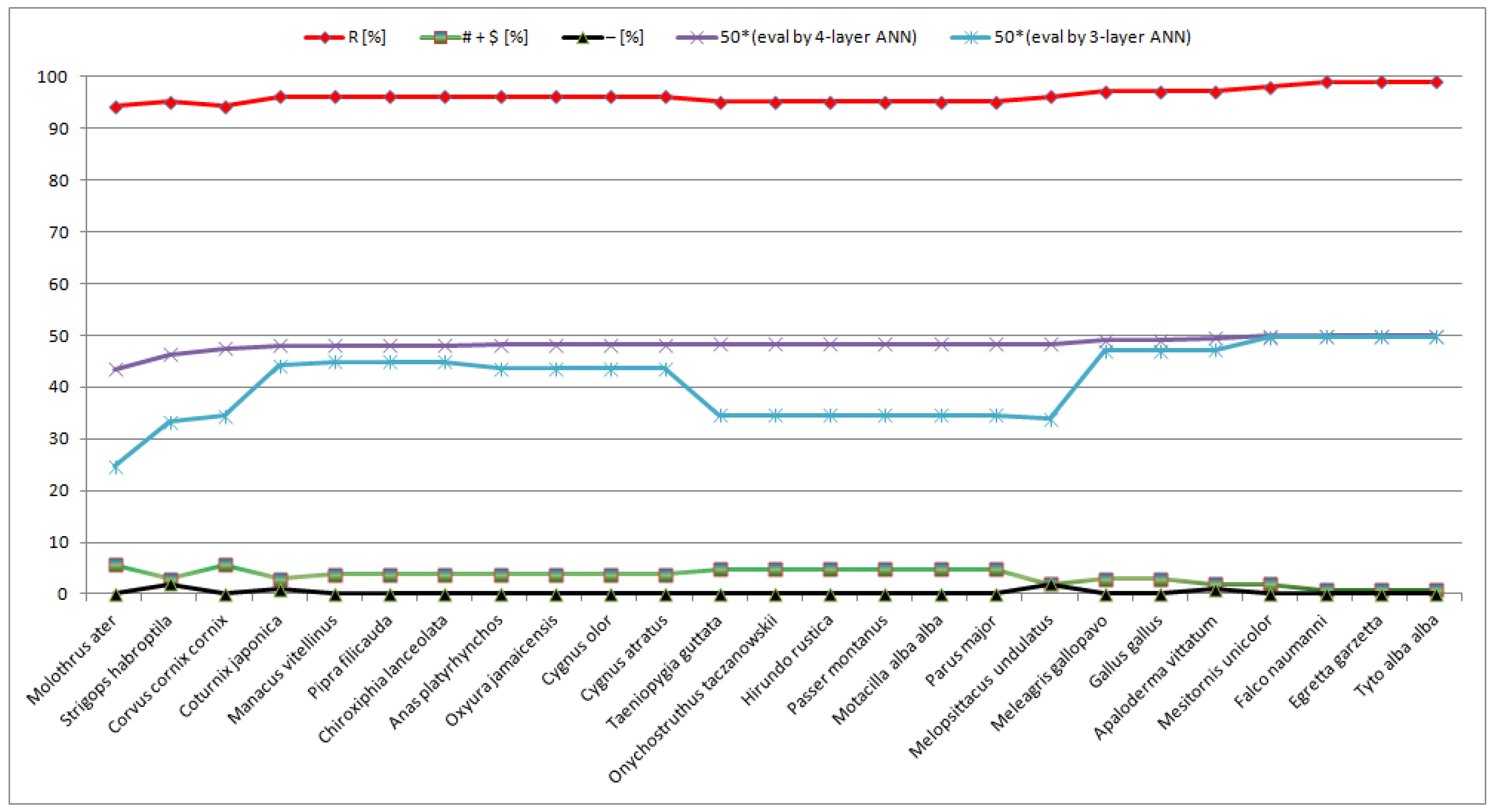
Selected representatives of birds have been checked in relation to Eagle (#13, Aquila chrysaetos chrysaetos). The results of calculations (i.e., recognized evolutionary similarities between Aquila chrysaetos chrysaetos and the selected representatives of birds by the three and four-layer neural networks and the number of homologous positions (i.e., “R” positions in [%]), semihomologous positions (i.e., sum of “#” and “$” positions in [%]), and the other positions (i.e., “-” positions in [%])) are presented in

Table A3. Evaluation of selected birds.

No.	Organism	Eval. by 4-Layer ANN	Eval. by 3-Layer ANN	[R/#/$/-]	R [%]	# + $ [%]	- [%]
1	Molothrus ater	0.87015	0.49342	[99/4/2/0]	94.29	5.71	0.00
2	Strigops habroptila	0.92589	0.66462	[99/2/1/2]	95.19	2.88	1.92
3	Corvus cornix cornix	0.94945	0.69007	[99/4/2/0]	94.29	5.71	0.00
4	Coturnix japonica	0.96097	0.88357	[101/2/1/1]	96.19	2.86	0.95
5	Manacus vitellinus	0.96223	0.89800	[101/1/3/0]	96.19	3.81	0.00
6	Pipra filicauda	0.96223	0.89800	[101/1/3/0]	96.19	3.81	0.00
7	Chiroxiphia lanceolata	0.96223	0.89800	[101/1/3/0]	96.19	3.81	0.00
8	Anas platyrhynchos	0.96240	0.87343	[101/2/2/0]	96.19	3.81	0.00
9	Oxyura jamaicensis	0.96240	0.87343	[101/2/2/0]	96.19	3.81	0.00
10	Cygnus olor	0.96240	0.87343	[101/2/2/0]	96.19	3.81	0.00
11	Cygnus atratus	0.96240	0.87343	[101/2/2/0]	96.19	3.81	0.00
12	Taeniopygia guttata	0.96549	0.69058	[100/3/2/0]	95.24	4.76	0.00
13	Onychostruthus taczanowskii	0.96549	0.69058	[100/3/2/0]	95.24	4.76	0.00
14	Hirundo rustica	0.96549	0.69058	[100/3/2/0]	95.24	4.76	0.00
15	Passer montanus	0.96549	0.69058	[100/3/2/0]	95.24	4.76	0.00
16	Motacilla alba alba	0.96549	0.69058	[100/3/2/0]	95.24	4.76	0.00
17	Parus major	0.96549	0.69058	[100/3/2/0]	95.24	4.76	0.00
18	Melopsittacus undulatus	0.96686	0.67747	[100/1/1/2]	96.15	1.92	1.92
19	Meleagris gallopavo	0.98139	0.93982	[102/2/1/0]	97.14	2.86	0.00
20	Gallus gallus	0.98139	0.93982	[102/2/1/0]	97.14	2.86	0.00
21	Apaloderma vittatum	0.99072	0.94316	[102/1/1/1]	97.14	1.90	0.95
22	Mesitornis unicolor	0.99760	0.99278	[103/1/1/0]	98.10	1.90	0.00
23	Falco naumanni	0.99826	0.99487	[104/1/0/0]	99.05	0.95	0.00
24	Egretta garzetta	0.99826	0.99487	[104/1/0/0]	99.05	0.95	0.00
25	Tyto alba alba	0.99826	0.99487	[104/1/0/0]	99.05	0.95	0.00

(see Appendix A) and in Figure 3.

The organisms presented in Figure 3 and in Table A3 (see Appendix A) have been set in the order of increasing evaluation by the four-layer neural network, i.e., in the order of increasing evolutionary similarities in relation to Aquila chrysaetos chrysaetos (#13). From Figure 3 and the results presented in Table A3 (see Appendix A), it is visible that the use of the neural networks (both the three and four-layer networks) allows the recognition of the bird-kind genome attractor (characterized by high average evaluations (i.e., high average evolutionary similarities) by the three and four-layer neural networks equal to 0.82162 and 0.96594, respectively). Additionally, to check this conclusion, the semihomologous approach has been applied. In this case, the use of the semihomologous approach also indicates the separation of birds (i.e., the big average number of “R” positions equal to 96.30 [%]) from the other organisms. Based on the results (Figure 3 and Table A3), a conclusion can be drawn that is presented as Remark 1.

Remark 1.

During evolution in this organism-kind genome attractor (indicated by increasing evolutionary similarities recognized by the four-layer neural network), the number of homologous positions (i.e., “R” positions) increases and the number of semihomologous positions (i.e., “# + $” positions) decreases, while the number of “-” positions remains small. It can be concluded that during evolution, semihomologous positions undergo changes to homologous positions, gradually increasing the number of homologous positions.

Selected representatives of fish have been checked in relation to Cod (#11, Gadus morhua). The results of calculations (i.e., recognized evolutionary similarities between Gadus morhua and the selected representatives of fishes by the three and four-layer neural networks and the number of homologous positions (i.e., “R” positions in [%]), semihomologous positions (i.e., sum of “#” and “$” positions in [%]), and the other positions (i.e., “-” positions in [%])) are presented in

Table A4. Evaluation of selected fish.

No.	Organism	Eval. by 4-Layer ANN	Eval. by 3-Layer ANN	[R/#/$/-]	R [%]	# + $ [%]	- [%]
1	Ictalurus furcatus	0.38863	0.21549	[93/6/4/1]	89.42	9.62	0.96
2	Danio rerio	0.70093	0.27851	[95/3/4/2]	91.35	6.73	1.92
3	Esox lucius	0.82171	0.90620	[98/1/3/2]	94.23	3.85	1.92
4	Cyprinodon tularosa	0.84813	0.86989	[94/3/6/1]	90.38	8.65	0.96
5	Fundulus heteroclitus	0.86372	0.56898	[93/3/5/3]	89.42	7.69	2.88
6	Larimichthys crocea	0.90449	0.65765	[97/1/3/3]	93.27	3.85	2.88
7	Simochromis diagramma	0.90905	0.74875	[94/2/6/2]	90.38	7.69	1.92
8	Pimephales promelas	0.95603	0.90426	[96/2/3/3]	92.31	4.81	2.88
9	Nothobranchius furzeri	0.96948	0.69571	[93/2/6/3]	89.42	7.69	2.88
10	Gasterosteus aculeatus aculeatus	0.97053	0.97994	[99/0/4/1]	95.19	3.85	0.96
11	Sander lucioperca	0.97813	0.93573	[99/0/3/2]	95.19	2.88	1.92
12	Megalops cyprinoides	0.98243	0.96318	[98/3/2/1]	94.23	4.81	0.96
13	Pungitius pungitius	0.98384	0.96021	[99/0/3/2]	95.19	2.88	1.92
14	Toxotes jaculatrix	0.98480	0.93835	[95/2/5/2]	91.35	6.73	1.92
15	Salmo salar	0.98535	0.97369	[97/3/1/3]	93.27	3.85	2.88
16	Xiphias gladius	0.98822	0.94512	[96/2/4/2]	92.31	5.77	1.92
17	Cheilinus undulatus	0.98853	0.97860	[97/4/1/2]	93.27	4.81	1.92
18	Oncorhynchus mykiss	0.98959	0.97672	[97/2/1/4]	93.27	2.88	3.85
19	Salvelinus namaycush	0.99351	0.98941	[98/1/4/1]	94.23	4.81	0.96
20	Acanthopagrus latus	0.99378	0.98557	[98/2/3/1]	94.23	4.81	0.96
21	Perca fluviatilis	0.99505	0.99017	[99/0/3/2]	95.19	2.88	1.92
22	Sebastes umbrosus	0.99563	0.99535	[99/1/2/2]	95.19	2.88	1.92
23	Amphiprion ocellaris	0.99675	0.99079	[99/1/1/3]	95.19	1.92	2.88
24	Oncorhynchus keta	0.99752	0.99548	[98/1/1/4]	94.23	1.92	3.85
25	Scophthalmus maximus	0.99756	0.99103	[98/1/3/2]	94.23	3.85	1.92

(see Appendix A) and in Figure 4.

The organisms presented in Figure 4 and in Table A4 (see Appendix A) have been set in the order of increasing evaluation by the four-layer neural network, i.e., in the order of increasing evolutionary similarities in relation to Gadus morhua (#11). From Figure 4 and the results presented in Table A4 (see Appendix A), it is visible that the use of the neural networks (both the three and four-layer networks) allows recognition of the fish-kind genome attractor (characterized by high average evaluations (i.e., high average evolutionary similarities) by the three and four-layer neural networks equal to 0.85739 and 0.92734, respectively). Additionally, to check this conclusion, the semihomologous approach has been applied. In this case, the use of the semihomologous approach also indicates the separation of fishes (i.e., the big average number of “R” positions equal to 93.04 [%]) from the other organisms. Oscillations of the number of “R”, “# + $”, and “-” positions can indicate a bigger variability of fishes in the fish-kind genome attractor, but the conclusion presented as Remark 1 is also valid in this case.

Standard deviation applied to the number of homologous (i.e., “R”), semihomologous (i.e., sum of “#” and “$” (i.e., “# + $”)), and “-” positions in the semihomologous approach has been calculated in order to check the variability of the selected organisms in their organism-kind genome attractors (

Table 4. Standard deviation applied to the number of homologous (i.e., “R”), semihomologous (“# + $”), and “-” positions in the semihomologous approach.

Organisms	Standard Deviation of the Number of
	R	# + $	-
Hominoids	0.447	0	0.447
OWM	0.667	0.782	0
NWM	0.877	0.65	0.65
Birds	1.485	1.497	0.597
Fish	2.087	2.235	0.898

).

The higher standard deviations obtained for fish indicate that the numbers of “R”, “# + $”, and “-” positions are spread out over a wider range (among the checked organisms) for these organisms (Table 4). This can also indicate that for the checked organisms, the variability of fishes in the fish-kind genome attractor is the highest. The evolutionary relationships recognized by the artificial neural networks are also characterized by the largest differences between the results obtained using the three and four-layer networks for fish. The variability of birds in the bird-kind genome attractor is smaller than the variability of fishes in the fish-kind genome attractor. Taking into account standard deviations of the number of “R” positions, the variability of hominoids in the hominoid-kind genome attractor is the smallest (Table 4). Based on these results, it can be concluded that more developed organisms show greater persistence (stability) in their organism-kind genome attractors. Since the real challenge is to find unambiguous intermediate transitional forms, for this reason, it can be concluded that organisms have been trapped in their organism-kind genome attractors eons ago. Being trapped in genome attractors, organisms undergo perturbations that drive microevolution. Looking at the multi-level organization of nature, most biologists are typically thinking that cause and effect events come from a lower (molecular) level of hierarchy of organization [45]. These events, in the form of perturbations, travel up this hierarchy [45]. Taking into account this point of view and in accordance with unified cell bioenergetics (UCB), the effects of bioenergetic disturbances (perturbations) can be depicted as shown in Figure 5.

In accordance with UCB, small disturbances (at molecular level) of cell bioenergetics can lead to small disturbances related, among others, to the Pasteur, Crabtree, Kluyver, and glucose effects; i.e., small disturbances can cause reversible effects (see Figure 5a). For example, these disturbances can be caused by a moderate ROS level that may affect a number of cell biological processes through transcriptional regulation (see Introduction). That means that small disturbances of cell bioenergetics can stimulate organism evolution without a change of genome attractor (i.e., can stimulate microevolution). However, huge or long-lasting (for example age-related) disturbances of cell bioenergetics can lead to specific diseases (including Alzheimer’s disease and cancer transformation) (see Figure 5b) [21,28]. The propagation of disturbances caused by a high level of ROS (resulting in severe oxidative damage to DNA, see Introduction) can also lead to changes of genome attractors by transformed cells [8].

4. Conclusions

In view of the presented results and conducted discussion, the following conclusions can be drawn:

• Sequences of cytochrome c, similarly to the sequences of cytochrome b, have written patterns that can be used to identify the evolution of organisms. In this work, it has been presented that these patterns can be recognized by artificial neural networks. Even small changes in the number of homologous positions and their distributions can be recognized by neural networks;
• The evolution analyzed on the basis of cytochrome c (and also cytochrome b) reveals a discontinuous character. Results obtained using the neural networks (both three and four-layer networks) point out that the analyzed groups of organisms (hominoids, OWM, NWM, birds, fish) are separated from each other, which may indicate that their evolution takes place in different organism-kind genome attractors (accordingly in hominoid-kind genome attractor, OWM-kind genome attractor, NWM-kind genome attractor, bird-kind genome attractor, and fish-kind genome attractor);
• Sequences of cytochrome c are much shorter compared to sequences of cytochrome b; for this reason, the use of cytochrome c allows the recognition of the patterns of organism evolution belonging to the attractors, but not so clearly as in the case of cytochrome b;
• The four-layer neural network usually more clearly recognized (comparing to the three-layer neural network) evolutionary similarities to the organisms that were used to train the neural networks. Using the language of attractors, the four-layer neural network more clearly recognized the affiliation of organisms to their organism-kind genome attractors;
• The variability of organisms in their organism-kind genome attractors depends on the development of organisms. Standard deviation applied to the number of “R”, “# + $”, and “-” positions (in the semihomologous approach) indicates that among the checked organisms, the most variable are fish, and the less variable are hominoids (Table 4). That can point out that hominoids, as the most developed among the checked organisms, are also the most stable in their organism-kind genome attractor. The consequence of the presented concept is the stabilization of the configuration of features typical for groups of highly developed organisms (for example, Old World Monkeys and hominoids) in different organism-kind genome attractors practically without the possibility of changing these attractors. That can indicate that the evolution of highly developed organisms occurs in their organism-kind genome attractors. On the other hand, primitive organisms can relatively easily change genome attractors. As an example, bacteria and also cells of developed multicellular organisms after the switch of cell-fate to cancerous cell-fate (i.e., atavistic cell-fate) can change genome attractors relatively easily (additionally, see [8]);
• In accordance with unified cell bioenergetics (UCB), disturbances (perturbations) of cell bioenergetics that lead to disturbances in the amount of NADH can be considered as a main driver of evolution.

References

1. Darwin, C. The Origin of Species; Oxford University Press: London, UK, 1859. [Google Scholar]
2. Gould, S.; Eldredge, N. Punctuated equilibrium comes of age. Nature 1993, 366, 223–227. [Google Scholar] [CrossRef] [PubMed]
3. Luo, D.; Huang, S. The genetic equidistance phenomenon at the proteomic level. Genomics 2016, 108, 25–30. [Google Scholar] [CrossRef]
4. Eldredge, N.; Gould, S.J. Punctuated equilibria: An alternative to phyletic gradualism. In Models in Paleobiology; Schopf, T.J.M., Ed.; Freeman. Cooper and Company: San Francisco, CA, USA, 1972. [Google Scholar]
5. Gould, S.J.; Eldredge, N. Punctuated Equilibria: The Tempo and Mode of Evolution Reconsidered. Paleobiology 1977, 3, 115–151. [Google Scholar] [CrossRef] [Green Version]
6. Ahad, A. The Direct Evidences (Paleontology/Fossils) of Evolution Opposite to Darwin’s Theory and Even Opposite to Human Evolution (Descent of Man) from the Lower Animal like Chimpanzee. Am. J. Life Sci. Res. 2015, 3, 56–76. [Google Scholar]
7. Vitas, M.; Dobovišek, A. Evolution, Transposition, Transformation and Flow of Information. Anali Pazu 2014, 4, 66–74. [Google Scholar]
8. Kasperski, A.; Kasperska, R. Study on attractors during organism evolution. Sci. Rep. 2021, 11, 9637. [Google Scholar] [CrossRef] [PubMed]
9. Lewin, R. Complexity: Life at the Edge of Chaos; Collier Books: Springfield, OH, USA, 1993. [Google Scholar]
10. Giuliani, A. Review of Thomas McCabe (ed.) 2021, Descente and Logic in Biosystematics. Juneau: Perseverant Publishing. Org. J. Biol. Sci. 2021, 5, 87–88. [Google Scholar] [CrossRef]
11. Kasperski, A.; Kasperska, R. A new approach to the automatic identification of organism evolution using neural networks. BioSystems 2016, 142–143, 32–42. [Google Scholar] [CrossRef] [PubMed]
12. Kasperski, A.; Kasperska, R. Application of n-dimensional dot-matrix to analysis of plant genetic diversity. Biul. IHAR 2015, 276, 69–83. [Google Scholar]
13. Kasperski, A.; Kasperska, R. Identifcation of protein family representatives. Curr. Bioinform. 2014, 9, 414–425. [Google Scholar] [CrossRef]
14. Kasperski, A.; Kasperska, R. A novel method of sequence similarity evaluation in n-dimensional sequence space. Curr. Bioinform. 2012, 7, 295–303. [Google Scholar] [CrossRef]
15. Zimatore, G.; Tsuchiya, M.; Hashimoto, M.; Kasperski, A.; Giuliani, A. Self-Organization of Whole Gene Expression Through Coordinated Chromatin Structural Transition: Validation of Self-Organized Critical Control of Genome Expression. BioRxiv 2019. [Google Scholar] [CrossRef] [Green Version]
16. Kumar, S. Molecular clocks: Four decades of evolution. Nat. Rev. Genet. 2005, 6, 654–662. [Google Scholar] [CrossRef] [PubMed]
17. Margoliash, E. Primary structure and evolution of cytochrome c. Proc. Natl. Acad. Sci. USA 1963, 50, 672–679. [Google Scholar] [CrossRef] [PubMed] [Green Version]
18. Keya, K.; Priya, S. A Study of Phylogenetic Relationships and Homology of Cytochrome C using Bioinformatics. Int. Res. J. Sci. Eng. 2016, 4, 65–75. [Google Scholar]
19. Kasperski, A.; Kasperska, R. Bioenergetics of life, disease and death phenomena. Theory Biosci. 2018, 137, 155–168. [Google Scholar] [CrossRef] [Green Version]
20. Kasperski, A.; Sun, K.; Tian, Y. New Approach to Control of the Dissolved Oxygen Concentration in a Biomass-Driven Self-Cycling Biochemical Process. Chem. Eng. Commun. 2016, 203, 75–93. [Google Scholar] [CrossRef]
21. Kasperski, A.; Kasperska, R. Selected disease fundamentals based on the unified cell bioenergetics. J. Investig. Biochem. 2013, 2, 93–100. [Google Scholar] [CrossRef]
22. Kasperski, A. Modelling of cells bioenergetics. Acta Biotheor. 2008, 56, 233–247. [Google Scholar] [CrossRef]
23. Kasperski, A.; Miśkiewicz, T. Optimization of pulsed feeding in a Baker’s yeast process with dissolved oxygen concentration as a control parameter. Biochem. Eng. J. 2008, 40, 321–327. [Google Scholar]
24. Kasperski, A.; Miśkiewicz, T. An adaptive fuzzy logic controller using the respiratory quotient as an indicator of overdosage in the baker’s yeast process. Biotechnol. Lett. 2002, 24, 17–21. [Google Scholar] [CrossRef]
25. Miśkiewicz, T.; Kasperski, A. A fuzzy logic controller to control nutrient dosage in a fed-batch baker’s yeast process. Biotechnol. Lett. 2000, 22, 1685–1691. [Google Scholar] [CrossRef]
26. Suchard, M.S.; Savulescu, D.M. Nicotinamide pathways as the root cause of sepsis – an evolutionary perspective on macrophage energetic shifts. FEBS J. 2021, 1–10. [Google Scholar] [CrossRef]
27. Alfarouk, K.O.; Verduzco, D.; Rauch, C.; Muddathir, A.K.; Bashir, A.H.H.; Elhassan, G.O.; Ibrahim, M.E.; Orozco, J.D.P.; Cardone, R.A.; Reshkin, S.J.; et al. Glycolysis, tumor metabolism, cancer growth and dissemination. A new pH-based etiopathogenic perspective and therapeutic approach to an old cancer question. Oncoscience 2014, 1, 777–802. [Google Scholar] [CrossRef] [PubMed]
28. Schwartz, L.; Henry, M.; Alfarouk, K.O.; Reshkin, S.J.; Radman, M. Metabolic Shifts as the Hallmark of Most Common Diseases: The Quest for the Underlying Unity. Int. J. Mol. Sci. 2021, 22, 3972. [Google Scholar] [CrossRef]
29. Cortassa, S.; Aon, M.A.; Winslow, R.L.; O’Rourke, B. A mitochondrial oscillator dependent on reactive oxygen species. Biophys. J. 2004, 87, 2060–2073. [Google Scholar] [CrossRef] [Green Version]
30. Damasco, A.; Giuliani, A. A resonance based model of biological evolution. Phys. A 2017, 471, 750–756. [Google Scholar] [CrossRef]
31. Harvey, P.H.; Pagel, M.D. The Comparative Method in Evolutionary Biology Vol. 239; Oxford University Press: Oxford, UK, 1991. [Google Scholar]
32. Heng, H.H. Debating Cancer: The Paradox in Cancer Research; World Scientific Publishing: Singapore, 2016; ISBN 978-981-4520-84-3. [Google Scholar]
33. Trachootham, D.; Alexandre, J.; Huang, P. Targeting cancer cells by ROS-mediated mechanisms: A radical therapeutic approach? Nat. Rev. Drug Discov. 2009, 8, 579–591. [Google Scholar] [CrossRef] [PubMed]
34. Trachootham, D.; Lu, W.; Ogasawara, M.A.; Nilsa, R.D.; Huang, P. Redox regulation of cell survival. Antioxid. Redox Sign. 2008, 10, 1343–1374. [Google Scholar] [CrossRef] [PubMed] [Green Version]
35. Heaton, J. Introduction to Neural Networks with Java, 1st ed.; Heaton Research, Inc.: St. Louis, MO, USA, 2005. [Google Scholar]
36. Masters, T. Practical Neural Network Recipes in C++; Academic Press: San Diego, CA, USA, 1993. [Google Scholar]
37. Leluk, J. A non-statistical approach to protein mutational variability. BioSystems 2000, 56, 83–93. [Google Scholar] [CrossRef]
38. Leluk, J. Regularities in mutational variability in selected protein families and the Markovian model of amino-acid replacement. J. Comput. Chem. 2000, 24, 659–672. [Google Scholar] [CrossRef]
39. Leluk, J.; Konieczny, L.; Roterman, I. Search for structural similarity in proteins. Bioinformatics 2003, 19, 117–124. [Google Scholar] [CrossRef]
40. Sumner, F.B. Is Evolution a Continuous or Discontinuous Process? Sci. Mon. 1929, 29, 72–78. [Google Scholar]
41. Hall, B.G. Phylogenetic Trees Made Easy; Oxford University Press Inc.: New York, NY, USA, 2017. [Google Scholar]
42. Munjal, G.; Hanmandlu, M.; Srivastava, S. Phylogenetics Algorithms and Applications. Ambient Commun. Comput. Sys. 2018, 904, 187–194. [Google Scholar] [CrossRef]
43. Xiong, J. Phylogenetic Tree Construction Methods and Programs. In Essential Bioinformatics; Cambridge University Press: Cambridge, UK, 2006; pp. 142–170. [Google Scholar] [CrossRef]
44. Kumar, S.; Stecher, G.; Li, M.; Knyaz, C.; Tamura, K. MEGA X: Molecular Evolutionary Genetics Analysis across Computing Platforms. Mol. Biol. Evol. 2018, 35, 1547–1549. [Google Scholar] [CrossRef] [PubMed]
45. Uversky, V.N.; Giuliani, A. Networks of Networks: An Essay on Multi-Level Biological Organization. Front. Genet. 2021, 12, 6260. [Google Scholar] [CrossRef]
Figure 1. The established order of the organisms from the most primitive (Bacteria (#1)) to the most developed organism (Rat (#19)) in relation to Homo sapiens (#20). The order has been established by calculating evolutionary distances and additionally using the semihomologous approach.
Processes 09 01646 g001
Figure 2. Evolution of New World Monkeys, Old World Monkeys, and hominoids examined in relation to Homo sapiens (#20) using the three and four-layer artificial neural networks (ANNs) and semihomologous approach.
Processes 09 01646 g002
Figure 3. Evolution of birds examined in relation to Aquila chrysaetos chrysaetos (#13) using the three and four-layer artificial neural networks (ANNs) and semihomologous approach.
Processes 09 01646 g003
Figure 4. Evolution of fish examined in relation to Gadus morhua (#11) using the three and four-layer artificial neural networks (ANNs) and semihomologous approach.
Processes 09 01646 g004
Figure 5. Disturbances (perturbations) of cell bioenergetics (CB) act (in view of unified cell bioenergetics) as a main driver of evolution that can lead to (a) reversible disturbances of cell bioenergetic effects and (b) specific diseases and also a change of genome attractor.
Processes 09 01646 g005