
Parallelization of a 3-Dimensional Hydrodynamics Model Using a Hybrid Method with MPI and OpenMP


Abstract
:1. Introduction
2. Materials and Methods
2.1. Research Trend in Parallel Calculation of EFDC Model
2.2. Development of Parallel Computational Code
2.3. Parallel Calculation Test Model Sets
3. Results and Discussion
3.1. Source Code Analysis for the EFDC-NIER Model
3.2. Parallel Performance Evaluation
3.3. Consistency Evaluation
4. Conclusions
- (1)
- The source code optimization and parallel code application resulted in a performance improvement by a factor of approximately five compared to the existing source code (Case 1). In the case of the existing EFDC, a large amount of time was consumed by a subroutine that wrote the results, and when this was improved, it took approximately half as much time for the calculation. As shown in Appendix B, the parallel calculation performance of the OpenMP and MPI methods applied in this study showed a similar level of performance as the results of the version developed and released by DSI. Therefore, the parallel calculation of the EFDC-NIER is better than or on par with that of the EFDC+ MPI, especially considering that its improvement values include the simulation results of the water quality factors.
- (2)
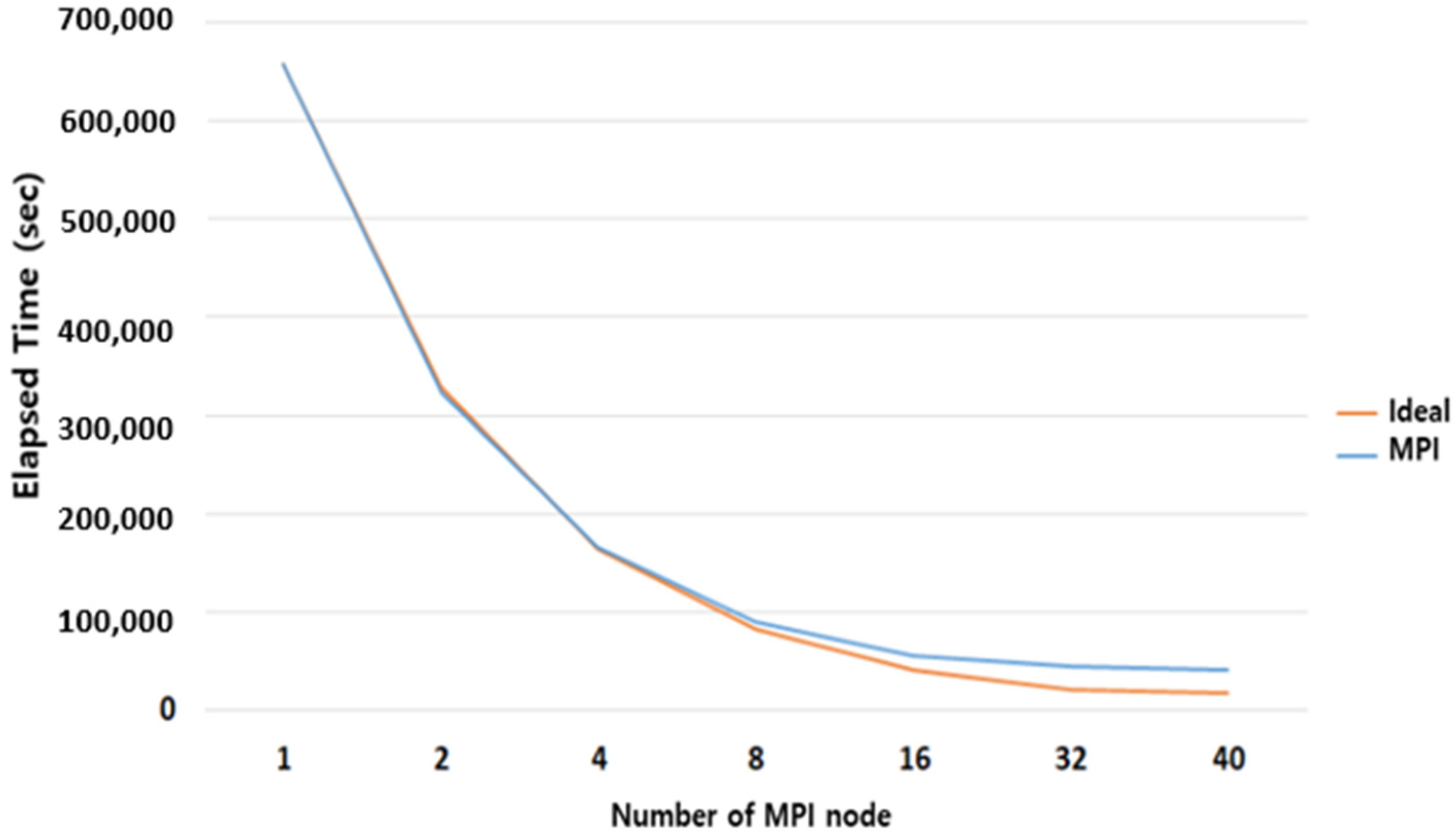
- For a Windows PC, there is no difference in the reduction of the calculation speed between the OpenMP and MPI methods because the core and thread resources are limited. However, as shown in Appendix C, when using a Linux server, the simulation is performed more ideally when the MPI method is used compared to the OpenMP method. In the case of the hybrid method that uses both the OpenMP and MPI methods, the optimal computing combination should be applied according to the performance and computing resources of the computer on which the simulation will be performed.
- (3)
- In the case of South Korea, algae prediction information for the water supply source sections of large rivers is sent to the water quality managers at eight-day intervals. When predicting the algae eight days into the future, all prediction work must be completed within 8 h. The fastest simulation’s calculation time (0.65 h) is a very important factor; if the optimization and the parallel computational source code applied in this study are used, quick calculation will be facilitated when urgent decision-making is required for an event such as a water pollution incident.
Author Contributions
Funding
Institutional Review Board Statement
Informed Consent Statement
Data Availability Statement
Acknowledgments
Conflicts of Interest
Appendix A

| Variables | Code Description | |
|---|---|---|
| Improved | IF (ISCFL.GE.1.AND.DEBUG) THEN IF (MYRANK.EQ.0) THEN OPEN (1, FILE = ‘CFL.OUT’, STATUS = ‘UNKNOWN’, POSITION = ‘APPEND’) ENDIF IF (MYRANK.EQ.0) THEN IF (ISCFL.EQ.1) WRITE (1,1212) DTCFL, N, ICFL, JCFL, KCFL IF (ISCFL.GE.2.AND.IVAL.EQ.0) WRITE (1,1213) IDTCFL ENDIF ENDIF |
| Conventional | DO NSP = 1, NXSP DO K = 1, KC; DO L = 2, LA WQ = WQVX(L, K, NSP) WRITE (95) WQ ENDDO; ENDDO ENDDO |
| Improved | DO NSP = 1, NXSP WRITE (95) WQVX (:,:,NSP) ENDDO |
| Category | Description |
|---|---|
| Sequential code | DO L = 2,LA RCG_R8(L) = CCC(L)*P(L) + CCS(L)*PSOUTH(L) + CCN(L)*PNORTH(L) & + CCW(L)*P(L-1) + CCE(L)*P(L + 1)-FPTMP(L) ENDDO DO L = 2,LA RS8Q = RS8Q + RCG_R8(L)*RCG_R8(L) ENDDO |
| Parallel code | !$OMP PARALLEL DO DO L = LMPI2,LMPILA RCG_R8(L) = CCC(L)*P(L) + CCS(L)*PSOUTH(L) + CCN(L)*PNORTH(L) & +CCW(L)*P(L-1) + CCE(L)*P(L + 1)-FPTMP(L) ENDDO !$OMP PARALLEL DO REDUCTION(+:RS8Q) DO L = LMPI2,LMPILA RS8Q = RS8Q + RCG_R8(L)*RCG_R8(L) ENDDO CALL MPI_ALLREDUCE(RS8Q,MPI_R8,1,MPI_DOUBLE, & MPI_SUM,MPI_COMM_WORLD,IERR) RS8Q = MPI_R8 |
Appendix B
| Category | EFDC-NIER | EFDC+ |
| Study area | Nakdong River | Chesapeake Bay |
| Number of horizontal grids | 116,473 | 204,000 |
| Vertical layers | 11 | 4 |
| Simulation factors | Hydraulics, water temperature, salinity, water quality, suspended sediments | Hydraulics, water temperature, salinity |
| CPU | Xeon E5-2650 v3 ×2 | Xeon Platinum 8000 Series |
| Number of cores | 10 (×2) | 36 |
| Number of nodes | 10 | 4 |
| Category | MPI Processor (Unit for Speed Improvement: Times) | |||
|---|---|---|---|---|
| 4 | 8 | 16 | 32 | |
| EFDC-NIER | 3.97 | 7.29 | 11.77 | 15.01 |
| EFDC+ | 4 | 7 | 11 | 17 |
Appendix C
| Category | Cluster | |
|---|---|---|
| CPU | Product | Intel Xeon CPU E5-2650 v3 * 2 ea |
| #Cores | 10 (Total 20) | |
| Frequency | 2.30 GHz | |
| Cache | 25 MB | |
| Instruction | 64-bit | |
| Extension | Intel AVX2 | |
| Memory | 64 GB | |
| OS | CentOS release 6.7 | |
| Network | InfiniBand ConnectX-3 VPI FDR, IB (56 Gb/s) | |
| Compiler | Intel Parallel Studio 2017.1.043 | |
| OpenMP | Intel OpenMP | |
| MPI | Intel MPI 2017.1.132 | |
- (1)
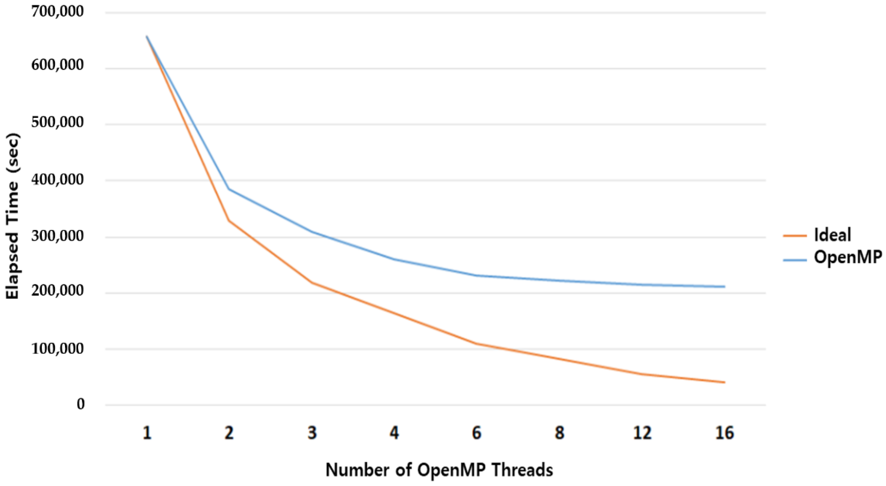
- OpenMP Parallel Performance Evaluation.
| Category | Number of OpenMP Threads | |||||||
|---|---|---|---|---|---|---|---|---|
| 01 | 02 | 03 | 04 | 06 | 08 | 12 | 16 | |
| HDMT2T | 656,953 | 385,124 | 308,917 | 259,871 | 231,408 | 221,675 | 215,195 | 210,575 |
| CALAVB | 21,823 | 11,475 | 8013 | 6445 | 5056 | 4282 | 3425 | 3083 |
| CALTSXY | 1722 | 1053 | 802 | 746 | 726 | 743 | 751 | 752 |
| CALEXP2T | 52,024 | 29,061 | 21,940 | 18,948 | 17,606 | 17,201 | 16,832 | 16,910 |
| CALCSER | 1006 | 1013 | 1148 | 1022 | 1059 | 1091 | 1088 | 1085 |
| CALPUV2C | 19,746 | 13,194 | 10,790 | 9814 | 9245 | 8976 | 8742 | 8842 |
| ADVANCE | 9040 | 7050 | 6393 | 6352 | 6367 | 6323 | 6266 | 6228 |
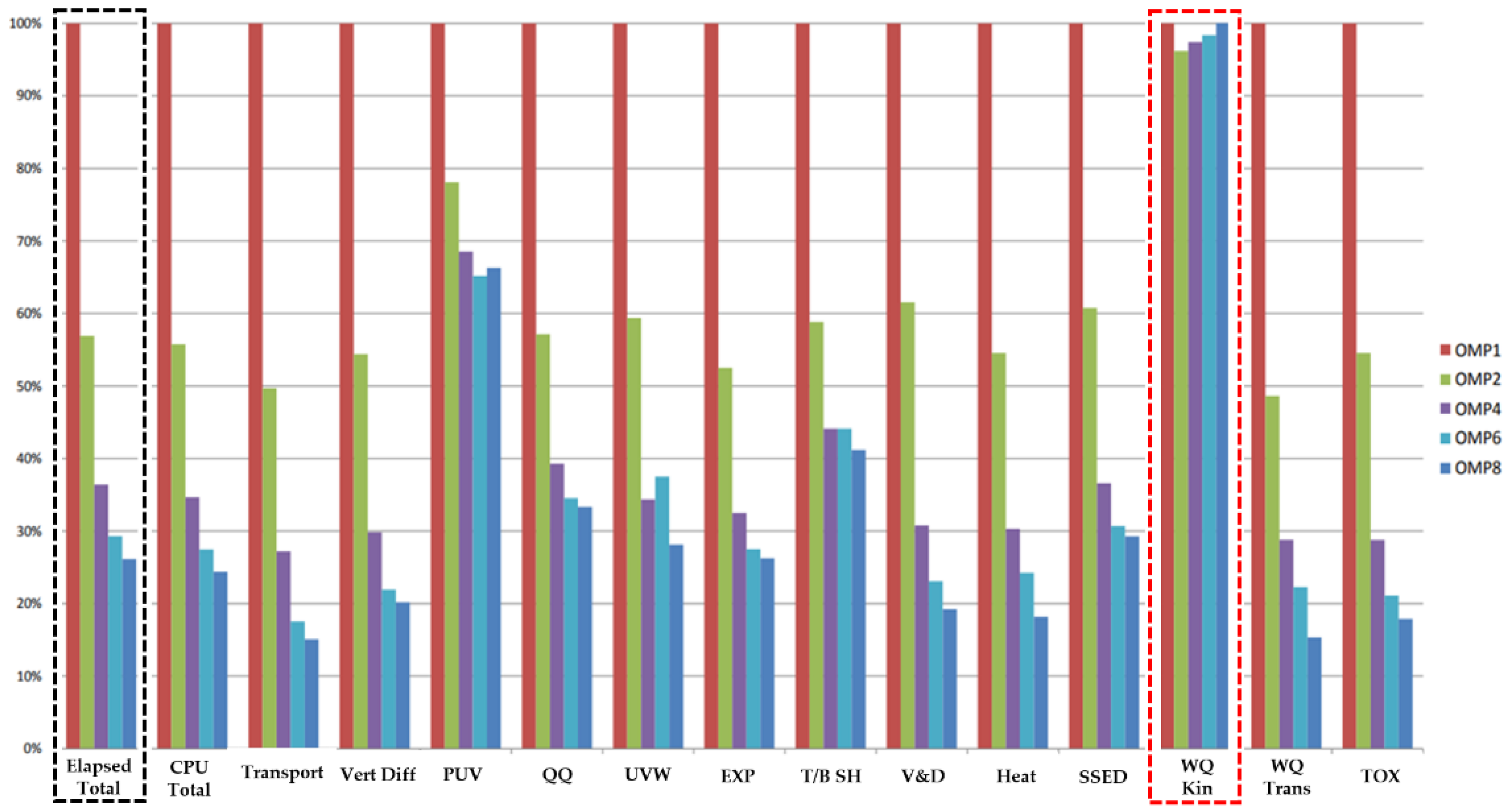
| CALUVW | 54,457 | 32,161 | 25,360 | 22,692 | 20,167 | 18,573 | 17,323 | 16,409 |
| CALCONC | 92,621 | 53,055 | 42,789 | 36,727 | 32,873 | 31,405 | 30,168 | 29,506 |
| SEDIMENT | 1931 | 1001 | 712 | 557 | 425 | 360 | 294 | 278 |
| WQ3D | 283,800 | 169,636 | 141,214 | 114,729 | 101,733 | 98,847 | 98,500 | 96,071 |
| CALBUOY | 6102 | 4293 | 3823 | 3716 | 3672 | 3619 | 3637 | 3691 |
| NLEVEL | 1781 | 971 | 678 | 549 | 486 | 489 | 491 | 505 |
| CALHDMF | 37,468 | 19,858 | 14,267 | 11,580 | 9188 | 8022 | 6687 | 6335 |
| CALTBXY | 10,391 | 5492 | 3768 | 2973 | 2278 | 1857 | 1446 | 1257 |
| QQSQR | 3063 | 1667 | 1199 | 997 | 786 | 673 | 559 | 555 |
| CALQQ2T | 55,889 | 29,635 | 21,593 | 17,561 | 15,242 | 14,577 | 14,262 | 14,231 |
| SURFPLT | 16 | 17 | 17 | 17 | 18 | 20 | 21 | 24 |
| VELPLTH | 38 | 37 | 38 | 37 | 39 | 43 | 48 | 55 |
| SALPTH | 726 | 824 | 827 | 861 | 864 | 878 | 862 | 883 |
| EEXPOUT | 3184 | 3499 | 3416 | 3423 | 3444 | 3448 | 3483 | 3536 |

- (2)
- MPI Parallel Performance Evaluation.
| Category | Number of MPI Nodes | ||||||
|---|---|---|---|---|---|---|---|
| 1 | 2 | 4 | 8 | 16 | 32 | 40 | |
| HDMT2T | 656,953 | 323,191 | 165,614 | 90,132 | 55,814 | 43,759 | 40,212 |
| CALAVB | 21,823 | 10,987 | 5606 | 2816 | 1435 | 857 | 703 |
| CALTSXY | 1722 | 860 | 487 | 290 | 179 | 124 | 108 |
| CALEXP2T | 52,024 | 25,490 | 12,655 | 6546 | 3541 | 2365 | 2006 |
| CALCSER | 1006 | 1018 | 995 | 1015 | 1122 | 1996 | 1936 |
| CALPUV2C | 19,746 | 9959 | 5517 | 3125 | 2020 | 1628 | 1733 |
| ADVANCE | 9040 | 4205 | 2126 | 1107 | 656 | 592 | 456 |
| CALUVW | 54,457 | 26,806 | 13,885 | 6912 | 3739 | 2350 | 1879 |
| CALCONC | 92,621 | 46,994 | 23,973 | 13,098 | 7977 | 7168 | 6571 |
| SEDIMENT | 1931 | 954 | 477 | 239 | 124 | 72 | 57 |
| WQ3D | 283,800 | 130,926 | 63,214 | 30,843 | 15,659 | 9898 | 8316 |
| CALBUOY | 6102 | 3123 | 1623 | 765 | 404 | 321 | 252 |
| NLEVEL | 1781 | 293 | 146 | 76 | 41 | 30 | 23 |
| CALHDMF | 37,468 | 17,835 | 12,250 | 9587 | 10,347 | 9145 | 9478 |
| CALTBXY | 10,391 | 4420 | 2206 | 1105 | 577 | 332 | 274 |
| QQSQR | 3063 | 1444 | 732 | 375 | 197 | 122 | 99 |
| CALQQ2T | 55,889 | 27,152 | 13,673 | 7129 | 3762 | 2349 | 1920 |
| SURFPLT | 16 | 18 | 17 | 17 | 17 | 19 | 19 |
| VELPLTH | 38 | 39 | 37 | 38 | 37 | 42 | 46 |
| SALPTH | 726 | 376 | 183 | 88 | 55 | 55 | 40 |
| EEXPOUT | 3184 | 3641 | 3474 | 3438 | 3481 | 3980 | 3988 |
| COMMUNICATION | 0 | 6606 | 2291 | 1497 | 413 | 278 | 272 |

- (3)
- Hybrid Parallel Performance Evaluation.
| Category | Hybrid (MPI + OpenMP) Combination (40 cpu) | |||||||
|---|---|---|---|---|---|---|---|---|
| MPI | OMP | MPI | OMP | MPI | OMP | MPI | OMP | |
| 4 | 10 | 8 | 5 | 20 | 2 | 40 | 1 | |
| HDMT2T | 54,457 | 39,300 | 41,800 | 40,212 | ||||
| CALAVB | 975 | 752 | 765 | 703 | ||||
| CALTSXY | 213 | 122 | 135 | 108 | ||||
| CALEXP2T | 3411 | 1921 | 2126 | 2006 | ||||
| CALCSER | 1078 | 1079 | 1307 | 1936 | ||||
| CALPUV2C | 3224 | 1724 | 2128 | 1733 | ||||
| ADVANCE | 1350 | 515 | 436 | 456 | ||||
| CALUVW | 3293 | 2283 | 2213 | 1879 | ||||
| CALCONC | 8102 | 5851 | 5816 | 6571 | ||||
| SEDIMENT | 155 | 88 | 73 | 57 | ||||
| WQ3D | 17,240 | 11,109 | 10,090 | 8316 | ||||
| CALBUOY | 1016 | 357 | 245 | 252 | ||||
| NLEVEL | 122 | 42 | 27 | 23 | ||||
| CALHDMF | 4039 | 5794 | 8882 | 9478 | ||||
| CALTBXY | 324 | 279 | 263 | 274 | ||||
| QQSQR | 152 | 104 | 100 | 98 | ||||
| CALQQ2T | 3738 | 2065 | 2295 | 1920 | ||||
| SURFPLT | 20 | 19 | 19 | 19 | ||||
| VELPLTH | 43 | 45 | 43 | 46 | ||||
| SALPTH | 178 | 57 | 32 | 40 | ||||
| EEXPOUT | 3625 | 3584 | 3516 | 3988 | ||||
| COMMUNICATION | 2101 | 1477 | 1256 | 272 | ||||
References
- Thornton, K.W.; Kimmel, B.L.; Payne, F.E. Reservoir Limnology-Ecological Perspectives; A Wiley Interscience Publication, John Wiley & Sons, Inc.: Hoboken, NJ, USA, 1990. [Google Scholar]
- Winston, W.E.; Criss, R.E. Geochemical variations during flash flooding, Meramec River basin. J. Hydrol. 2000, 265, 149–163. [Google Scholar] [CrossRef]
- You, K.A.; Byeon, M.S.; Hwang, S.J. Effects of hydraulic-hydrological changes by monsoon climate on the zooplankton community in lake Paldang, Korea. Korean J. Limnol. 2012, 45, 278–288. [Google Scholar]
- Jung, W.S.; Kim, Y.D. Effect of abrupt topographical characteristic change on water quality in a river. KSCE J. Civ. Eng. 2019, 23, 3250–3263. [Google Scholar] [CrossRef]
- Bomers, M.; Schielen, R.M.J.; Hulscher, S.J.M.H. The influence of grid shape and grid size on hydraulic river modelling performance. Environ. Fluid Mech. 2019, 19, 1273–1294. [Google Scholar] [CrossRef] [Green Version]
- Avesani, D.; Galletti, A.; Piccolroaz, S.; Bellin, A.; Majone, B. A dual-layer MPI continuous large-scale hydrological model including Human Systems. Environ. Model. Softw. 2021, 139, 105003. [Google Scholar] [CrossRef]
- Neal, J.; Fewtrell, T.; Bates, P.; Wright, N. A comparison of three parallelisation methods for 2D flood inundation models. Environ. Model. Softw. 2010, 25, 398–411. [Google Scholar] [CrossRef]
- Rouholahnejad, E.; Abbaspour, K.C.; Vejdani, M.; Srinivasan, R.; Schulin, R.; Lehmann, A. A parallelization framework for calibration of hydrological models. Environ. Model. Softw. 2012, 31, 28–36. [Google Scholar] [CrossRef]
- Liu, J.; Zhu, A.X.; Liu, Y.; Zhu, T.; Qin, C.Z. A layered approach to parallel computing for spatially distributed hydrological modeling. Environ. Model. Softw. 2014, 51, 221–227. [Google Scholar] [CrossRef]
- Neal, J.; Fewtrell, T.; Trigg, M. Parallelisation of storage cell flood models using OpenMP. Environ. Model. Softw. 2009, 24, 872–877. [Google Scholar] [CrossRef]
- Lawrence Livermore National Laboratory. Available online: https://computing.llnl.gov/tutorials/parallel_comp/ (accessed on 5 April 2021).
- Gropp, W.; Lusk, E.; Doss, N.; Skjellum, A. A high-performance, portable implementation of the MPI message passing interface standard. Parallel Comput. 1996, 22, 789–828. [Google Scholar] [CrossRef]
- Chapman, B.; Jost, G.; Van Der Paas, R. Using OpenMP: Portable Shared Memory Parallel Programming; MIT Press: Cambridge, MA, USA, 2007. [Google Scholar]
- Eghtesad, A.; Barrett, T.J.; Germaschewski, K.; Lebensohn, R.A.; McCabe, R.J.; Knezevic, M. OpenMP and MPI implementations of an elasto-viscoplastic fast Fourier transform-based micromechanical solver for fast crystal plasticity modeling. Adv. Eng. Softw. 2018, 126, 46–60. [Google Scholar] [CrossRef]
- Jiao, Y.; Zhao, Q.; Wang, L.; Huang, G.; Tan, F. A hybrid MPI/OpenMP parallel computing model for spherical discontinuous deformation analysis. Comput. Geotech. 2019, 106, 217–227. [Google Scholar] [CrossRef]
- Ouro, P.; Fraga, B.; Lopez-Novoa, U.; Stoesser, T. Scalability of an Eulerian-Lagrangian large-eddy simulation solver with hybrid MPI/OpenMP parallelisation. Comput. Fluids 2019, 179, 123–136. [Google Scholar] [CrossRef]
- Zhou, H.; Tóth, G. Efficient OpenMP parallelization to a complex MPI parallel magnetohydrodynamics code. J. Parallel Distrib. Comput. 2020, 139, 65–74. [Google Scholar] [CrossRef]
- Klinkenberg, J.; Samfass, P.; Bader, M.; Terboven, C.; Müller, M.S. Chameleon: Reactive load balancing for hybrid MPI + OpenMP task-parallel applications. J. Parallel Distrib. Comput. 2020, 138, 55–64. [Google Scholar] [CrossRef]
- Stump, B.; Plotkowski, A. Spatiotemporal parallelization of an analytical heat conduction model for additive manufacturing via a hybrid OpenMP + MPI approach. Comput. Mater. Sci. 2020, 184, 109861. [Google Scholar] [CrossRef]
- Zhao, Z.; Ma, R.; He, L.; Chang, X.; Zhang, L. An efficient large-scale mesh deformation method based on MPI/OpenMP hybrid parallel radial basis function interpolation. Chin. J. Aeronaut. 2020, 33, 1392–1404. [Google Scholar] [CrossRef]
- Noh, S.J.; Lee, J.H.; Lee, S.; Kawaike, K.; Seo, D.J. Hyper-resolution 1D-2D urban flood modelling using LiDAR data and hybrid parallelization. Environ. Model. Softw. 2018, 103, 131–145. [Google Scholar] [CrossRef]
- Stacey, M.W.; Pond, S.; Nowak, Z.P. A numerical model of circulation in Knight Inlet, British Columbia, Canada. J. Phys. Oceanogr. 1995, 25, 1037–1062. [Google Scholar] [CrossRef] [Green Version]
- Adcroft, A.; Campin, J.M. Rescaled height coordinates for accurate representation of free-surface flows in ocean circulation models. Ocean Model. 2004, 7, 269–284. [Google Scholar] [CrossRef]
- Tetra Tech. EFDC Technical Memorandum. Theoretical and Computational Aspects of the Generalized Vertical Coordinate Option in the EFDC Model; Tetra Tech, Inc.: Fairfax, VA, USA, 2007. [Google Scholar]
- Tetra Tech. The Environmental Fluid Dynamics Code, User Manual, US EPA Version 1.01; Tetra Tech, Inc.: Fairfax, VA, USA, 2007. [Google Scholar]
- Ahn, J.M.; Kim, J.; Park, L.J.; Jeon, J.; Jong, J.; Min, J.H.; Kang, T. Predicting cyanobacterial harmful algal blooms (CyanoHABs) 2 in a regulated river using a revised EFDC model. Water 2021, 13, 439. [Google Scholar] [CrossRef]
- Ahn, J.M.; Kim, B.; Jong, J.; Nam, G.; Park, L.J.; Park, S.; Kang, T.; Lee, J.K.; Kim, J. Predicting cyanobacterial blooms using hyperspectral images in a regulated river. Sensors 2021, 21, 530. [Google Scholar] [CrossRef]
- Hamrick, J.M. A Three-Dimensional Environmental Fluid Dynamics Computer Code: Theoretical and Computational Aspects. In Applied Marine Science and Ocean Engineering; Special Report No. 317; Virginia Institute of Marine Science: Gloucester Point, VA, USA, 1992; p. 58. [Google Scholar]
- Craig, P.M. Users Manual for EFDC_Explorer: A Pre/Post Processor for the Environmental Fluid Dynamics Code, Ver 160307; DSI LLC: Edmonds, WA, USA, 2016. [Google Scholar]
- DSI. EFDC_DSI/EFDC_Explorer Modeling System, Use and Applications for Alberta ESRD Environmental Modelling Workshop; DSI LLC: Edmonds, WA, USA, 2013. [Google Scholar]
- O’Donncha, F.; Ragnoli, E.; Suits, F. Parallelisation study of a three-dimensional environmental flow model. Comput. Geosci. 2014, 64, 96–103. [Google Scholar] [CrossRef]
- GitHub EFDC-MPI. Available online: https://github.com/fearghalodonncha/EFDC-MPI (accessed on 12 April 2021).
- Kwedlo, W.; Czochanski, P.J. A hybrid MPI/OpenMP parallelization of K-means algorithms accelerated using the triangle inequality. IEEE Access 2019, 7, 42280–42297. [Google Scholar] [CrossRef]
- Gropp, W.; Hoefler, T.; Thakur, R.; Lusk, E. Using Advanced MPI: Modern Features of the Message-Passing Interface; MIT Press: Cambridge, MA, USA, 2014. [Google Scholar]
- Mausolff, Z.; Craig, P.; Scandrett, K.; Mishra, A.; Lam, N.T.; Mathis, T. EFDC + Domain Decomposition: MPI-Based Implementation; DSI LLC: Edmonds, WA, USA, 2020. [Google Scholar]
- Amdahl, G.M. Validity of the single processor approach to achieving large scale computing capabilities. In Proceedings of the AFIPS Conference, Atlantic city, NJ, USA, 18–20 April 1967; AFIPS Press: Reston, VA, USA, 1967; Volume 30, pp. 483–485. [Google Scholar]


| Function | Description |
|---|---|
| MPI_INITIALIZE | Initializes MPI and sets up MPI variables (number of nodes, rank of each node) |
| MPI_DECOMPOSITION | Partitions the LA index |
| BROADCAST_BOUNDARY | Performs communication of boundary values between MPI nodes (1D variable) |
| BROADCAST_BOUNDARY_ARRAY | Performs communication of boundary values between MPI nodes (2D and 3D) |
| COLLECT_IN_ZERO | Performs collective communication to send the variables to the master node (1D) |
| COLLECT_IN_ZERO_ARRAY | Performs collective communication to send the variables to the master node (2D and 3D) |
| MPI_TIC/MPI_TOC | Timestamp for hotspot analysis (MPI Walltime) |
| Case | Description | Comparison Method | |
|---|---|---|---|
| Case 1 | Before optimization and parallel code application | Consistency of calculation times and results for simulations from 1 July 2015 to 9 July 2015 | |
| Case 2 | 1 | Sequential code optimization | |
| 2 | Case 2-1 + Changed method of writing the result file | ||
| Case 3 | Case 2-2 + OpenMP (6 threads) | ||
| Case 4 | Case 2-2 + MPI (6 nodes) | ||
| Case 5 | 1 | Case 2-2 + Hybrid (1 thread + 5 nodes) | |
| 2 | Case 2-2 + Hybrid (2 threads + 4 nodes) | ||
| 3 | Case 2-2 + Hybrid (3 threads + 3 nodes) | ||
| 4 | Case 2-2 + Hybrid (4 threads + 2 nodes) | ||
| 5 | Case 2-2 + Hybrid (5 threads + 1 node) | ||
| Category | Description | |
|---|---|---|
| Model | Number of grids | Horizontal: 6998 units, vertical: 11 layers |
| Windows PC | CPU | Inter Core i7-8700 3.20 GHz, 6 cores |
| Memory | 32 GB | |
| OS | Microsoft Windows 10 Pro 64-bit | |
| Compiler | Intel parallel studio XE 2020, 19.1.2.254 20200623 | |
| Function Name | Description | Proportion of Execution Time (%) |
|---|---|---|
| HDMT2T | Main code of numerical simulation | 100.00 |
| WQ3D | Water quality component simulation | 38.03 |
| CALUVW | Flow rate/direction component simulation | 18.45 |
| CALCONC | Concentration (water temperature, sediment) simulation | 10.65 |
| CALQQ2T | Turbulence intensity simulation | 7.33 |
| CALEXP2T | Explicit momentum equation calculation | 6.17 |
| CALHDMF | Simulation of horizontal viscosity and spreading momentum | 4.66 |
| CALPUV2C | Simulation of surface P, UHDYE, and VHDXE | 4.12 |
| EEXPOUT | Writing a result file | 3.15 |
| CALAVB | Simulation of vertical viscosity and dispersion | 3.12 |
| ADVANCE | Updating the next timestep value | 0.98 |
| CALBUOY | Buoyancy simulation | 0.98 |
| CALTBXY | Bottom friction factor calculation | 0.60 |
| QQSQR | Updating the turbulence intensity value | 0.56 |
| CALCSER | Updating the boundary data | 0.35 |
| CALTSXY | Updating the surface wind stress | 0.28 |
| SEDIMENT | Sediment simulation | 0.25 |
| NLEVEL | Distribution of variables for each timestep | 0.11 |
| SALPTH | Writing the salinity result | 0.09 |
| DUMP | Recording the model variable dump | 0.06 |
| Case | Simulation Time (h) | |
|---|---|---|
| Case 1 | 3.22 | |
| Case 2 | 1 | 2.68 |
| 2 | 1.69 | |
| Case 3 | 0.74 | |
| Case 4 | 0.69 | |
| Case 5 | 1 | 0.66 |
| 2 | 0.73 | |
| 3 | 0.68 | |
| 4 | 0.65 | |
| 5 | 0.79 | |
| Variable | Case 1 | Case 3 | Case 4 |
|---|---|---|---|
| TSX | 6.173959 × 10⁻⁴ | 6.173959 × 10⁻⁴ | 6.173959 × 10⁻⁴ |
| TSY | 6.763723 × 10⁻⁴ | 6.763723 × 10⁻⁴ | 6.763723 × 10⁻⁴ |
| TBX | 2.715987 × 10⁻² | 2.715987 × 10⁻² | 2.715987 × 10⁻² |
| TBY | 3.796839 × 10⁻¹ | 3.796839 × 10⁻¹ | 3.796839 × 10⁻¹ |
| AV | 6.224335 | 6.224335 | 6.224335 |
| AB | 7.667015 | 7.667015 | 7.667015 |
| AQ | 2.551961 | 2.551961 | 2.551961 |
| HP | 3.046219 × 10⁴ | 3.046219 × 10⁴ | 3.046219 × 10⁴ |
| HU | 3.080725 × 10⁴ | 3.080725 × 10⁴ | 3.080725 × 10⁴ |
| HV | 3.018550 × 10⁴ | 3.018550 × 10⁴ | 3.018550 × 10⁴ |
| P | 1.726112 × 10⁶ | 1.726112 × 10⁶ | 1.726112 × 10⁶ |
| U | 1.927491 × 10² | 1.927491 × 10² | 1.927491 × 10² |
| V | 1.632354 × 10³ | 1.632354 × 10³ | 1.632354 × 10³ |
| W | 8.197821 × 10⁻¹ | 8.197821 × 10⁻¹ | 8.197821 × 10⁻¹ |
| TEM | 1.677452 × 10⁵ | 1.677452 × 10⁵ | 1.677452 × 10⁵ |
| SEDT | 4.259870 × 10⁵ | 4.259870 × 10⁵ | 4.259870 × 10⁵ |
| 1.507725 × 10 | 1.507725 × 10 | 1.507725 × 10 | |
| QQL | 1.070996 | 1.070996 | 1.070996 |
| WQV | 2.552020 × 10⁵ | 2.552020 × 10⁵ | 2.552020 × 10⁵ |
| WQVX | 5.815869 × 10⁴ | 5.815869 × 10⁴ | 5.815869 × 10⁴ |
| Date | Case 1 | Case 3 | Case 4 | Case 5-4 | ||||||||
|---|---|---|---|---|---|---|---|---|---|---|---|---|
| BOD | T-N | T-P | BOD | T-N | T-P | BOD | T-N | T-P | BOD | T-N | T-P | |
| 01-07-2015 | 1.453 | 3.590 | 0.080 | 1.453 | 3.590 | 0.080 | 1.453 | 3.590 | 0.080 | 1.453 | 3.590 | 0.080 |
| 02-07-2015 | 1.481 | 3.609 | 0.079 | 1.481 | 3.609 | 0.079 | 1.481 | 3.609 | 0.079 | 1.481 | 3.609 | 0.079 |
| 03-07-2015 | 1.521 | 3.658 | 0.080 | 1.521 | 3.658 | 0.080 | 1.521 | 3.658 | 0.080 | 1.521 | 3.658 | 0.080 |
| 04-07-2015 | 1.547 | 3.700 | 0.081 | 1.547 | 3.700 | 0.081 | 1.547 | 3.700 | 0.081 | 1.547 | 3.700 | 0.081 |
| 05-07-2015 | 1.520 | 3.712 | 0.079 | 1.520 | 3.712 | 0.079 | 1.520 | 3.712 | 0.079 | 1.520 | 3.712 | 0.079 |
| 06-07-2015 | 1.596 | 3.672 | 0.081 | 1.596 | 3.672 | 0.081 | 1.596 | 3.672 | 0.081 | 1.596 | 3.672 | 0.081 |
| 07-07-2015 | 1.637 | 3.612 | 0.080 | 1.637 | 3.612 | 0.080 | 1.637 | 3.612 | 0.080 | 1.637 | 3.612 | 0.080 |
| 08-07-2015 | 1.563 | 3.568 | 0.081 | 1.563 | 3.568 | 0.081 | 1.563 | 3.568 | 0.081 | 1.563 | 3.568 | 0.081 |
| 09-07-2015 | 1.634 | 3.493 | 0.081 | 1.634 | 3.493 | 0.081 | 1.634 | 3.493 | 0.081 | 1.634 | 3.493 | 0.081 |
Publisher’s Note: MDPI stays neutral with regard to jurisdictional claims in published maps and institutional affiliations. |
© 2021 by the authors. Licensee MDPI, Basel, Switzerland. This article is an open access article distributed under the terms and conditions of the Creative Commons Attribution (CC BY) license (https://creativecommons.org/licenses/by/4.0/).
Share and Cite
Ahn, J.M.; Kim, H.; Cho, J.G.; Kang, T.; Kim, Y.-s.; Kim, J. Parallelization of a 3-Dimensional Hydrodynamics Model Using a Hybrid Method with MPI and OpenMP. Processes 2021, 9, 1548. https://doi.org/10.3390/pr9091548
Ahn JM, Kim H, Cho JG, Kang T, Kim Y-s, Kim J. Parallelization of a 3-Dimensional Hydrodynamics Model Using a Hybrid Method with MPI and OpenMP. Processes. 2021; 9(9):1548. https://doi.org/10.3390/pr9091548
Chicago/Turabian StyleAhn, Jung Min, Hongtae Kim, Jae Gab Cho, Taegu Kang, Yong-seok Kim, and Jungwook Kim. 2021. "Parallelization of a 3-Dimensional Hydrodynamics Model Using a Hybrid Method with MPI and OpenMP" Processes 9, no. 9: 1548. https://doi.org/10.3390/pr9091548
APA StyleAhn, J. M., Kim, H., Cho, J. G., Kang, T., Kim, Y.-s., & Kim, J. (2021). Parallelization of a 3-Dimensional Hydrodynamics Model Using a Hybrid Method with MPI and OpenMP. Processes, 9(9), 1548. https://doi.org/10.3390/pr9091548