Quantitative Analysis Regarding the Incidents to the Pipelines of Petroleum Products for an Efficient Use of the Specific Transportation Infrastructure

Abstract

The transportation infrastructure for petroleum products contains complex pipeline systems, developed on a global scale and totaling investments of hundreds of millions of dollars. The operation and maintenance of these systems have to be performed in relation to the analysis of incidents of various types, which take place in various areas of the world. The present paper aims to analyze in as much detail as possible, from a statistical point of view, the case of the pipeline system for petroleum products in Romania in order to streamline the operation of this critical infrastructure for Romania. Through the statistical tools, we established the hierarchies of the causes of the analyzed incidents, weights of the effects generated by these sources of accidents, and correlations between various parameters, in order to create a useful plan of measures and actions in the efficient operation of the pipeline system. The importance and topicality of the subject is also demonstrated by the major negative impact of the accidents in this sector, through product leaks from pipes in the soil and in watercourses, which generate significant pollution values, thus influencing the balance of the environment.

1. Introduction

The world’s oil and gas pipeline system covers hundreds and thousands of miles. This has been conducted as a major investment for areas or countries that do not have such resources to benefit from their processing. These investments have now become a priority for companies that own these pipelines, as incidents have begun to occur and it is necessary to monitor and manage such situations. Incidents such as accidents, breakdowns, or failures are unfortunate events because of the consequences they entail: in some cases, the consequences can be economic, environmental or, in the worst conditions imaginable, accidents that can cause loss of life [1]. Pipeline safety and integrity are crucial for a sustainable future and responsible development [2]. Precisely out of the desire to ensure increased safety in the transport of petroleum products, it is necessary to analyze in as much detail as possible the causes of incidents produced over time.

Basically, the main question for this study is: what are the main causes in the generation of incidents in the pipeline system of petroleum products? This must be ascertained in order to design appropriate measures and actions, including maintenance solutions, to make the specific transport infrastructure more efficient and less polluting.

Therefore, this study identifies the main factors and causes of incidents for the pipeline system of petroleum products in Romania. Available data from 2017 to 2019 are statistically analyzed. There are generated hierarchies for causes of incidents, and correlations are checked for different parameters, related to the pipeline incidents. The analysis is necessary for the implementation of a plan of measures to include: investments in equipment and for the replacement of some sections of pipes that have been affected; protection of lands that have pipes in their basement; complex measures for monitoring areas that have pipelines; updated maintenance plans, etc.

The causes of oil spills must be known, analyzed, and treated in order to eliminate the loss of oil products through pipeline systems and protect the environment.

There are various databases around the world related to pipeline incidents in the transportation of petroleum products, as follows:

-

In the US, Pipeline and Hazardous Materials Safety Administration (PHMSA);

-

In Canada, Pipeline Incident Database (PID);

-

In the United Kingdom, United Kingdom Onshore Pipeline Operators’ Associations (UKOPA);

-

In Europe, European Gas Pipeline Incident Data Group (EGIG);

-

In Russia, initially National Technical Inspectorate and then Federal Service for Environmental, Technological and Nuclear Supervision; and

-

In Australia, Australian Pipeline Industry Association (APIA).

Most countries in the world (including Romania) do not have a database system for reporting oil and gas pipeline incidents. Why would a globally unified database be needed? Because each database, at regional or national level, contains different criteria for reporting incidents in this category. In addition, the presentation and debate of cases declared at the level of certain areas or countries must be conducted through the prism of common, standardized elements and must be unanimously accepted by experts.

In addition, there are organizations and associations that specialize in conducting studies dedicated to this sector. One such globally recognized and representative entity is the European Oil Company Organisation for Environment, Health and Safety (CONCAWE). CONCAWE, a European association that includes a group of leading oil companies (more than 40), carries out regular research on environmental issues relevant to the oil industry. The topics cover wide areas, such as: fuel quality and emissions, air quality, water quality, waste, soil contamination, cross-country pipeline performance, etc.

At the same time, some specialists describe, in a simplified way, the causes of pipeline failure. For example, a classification was proposed with four sources of incidents [3]:

-

Third-party damage;

-

Corrosion;

-

Design and construction error; and

-

Incorrect operation conditions.

In order to demonstrate the lack of unity of points of view in classifying the causes of pipeline incidents, two of the most representative databases are presented: PHMSA and EGIG.

PHMSA database proposes a system that contains eight categories of pipeline failure causes: corrosion (external; internal; stress corrosion cracking; selective seam corrosion); excavation damage; natural force damage; material/weld failure; equipment failure; incorrect operation; and all other causes. EGIG database has a classification that contains only five categories: corrosion; external interference; construction defect/material failure; ground movements; other and unknown.

In the US, pipeline operators are required by law to report pipeline incidents, while in Europe this is not mandatory.

The importance of the subject is demonstrated by the fact that such accidents incur high material costs for the oil pipeline’s operating companies and significant damage to the environment, people, and property in the vicinity of the pipeline failures.

The topicality of the studied topic is proven by the provision of information based on the content of the PHMSA database in the period 2010–2020 (

Table 1. Summary of pipeline incidents in the US from 2010 to 2020 (authors’ own processing from PHMSA database).

Report	Incidents	Injuries	Fatalities	Evacuees	Fires	Explosions	Damages ($)
Gas Distribution	1222	539	115	27,870	714	273	2,408,976,046
Gas Transmission & Gathering	1369	110	27	13,153	146	63	1,492,746,535
Hazardous Liquids	4359	39	14	2780	145	19	2,962,900,530
Totals	6950	688	156	43,803	1005	355	6,864,623,111

). From these data, it is easy to deduce the major negative effect produced by these incidents from the point of view of the affected persons, on the environment and from a financial point of view.

On the other hand, at present, the Romanian national company operates a pipeline transport system with a length of 3809 km, of which 3161 km (82% of the total) is actually used for the transport of crude oil, gasoline, condensate, and liquid ethane. The action area is located mainly in the southern part of the country and with a direct connection to the main port on the Black Sea, Constanta.

The crude oil transport via pipelines in Romania has a history of over 115 years. In 1901, the first crude oil transport via pipelines in Romania was along the route Buştenari-Băicoi Rail Station, Prahova County. Today, the company transports crude oil via the national pipeline system describing 3800 km in length and 27 million tons’ throughput, crossing 24 counties. The maximum allowable losses during transportation are <0.365% from the total transported quantity; otherwise, the company should pay taxes due to the losses incurred and environmental pollution.

Therefore, the crude oil transport activity must be carefully monitored so that the number of incidents in the pipeline system decreases and the negative impact, generated by these incidents, manifests itself on a much smaller scale.

The paper is designed in a standard way, so that after the Introduction, Section 2 is dedicated to Literature Review, then Section 3, entitled Materials and Methods, is integrated, followed by Section 4 for Results, and finally, Section 5, containing Conclusions, is included.

2. Literature Review

The pipelines are considered the safest way to transport petroleum products [4]. Actually, the idea of using pipelines to transport hazardous products as a preferred method is related to the safety and cost, when compared to train and ground transportation [5]. Still, the pipeline systems are associated with risks, leading to negative consequences [6,7].

Oil spills are environmental disasters and their long-term impact is not just a concern for the environment and economy, but also for health and well-being of all living things [8]. Moreover, along with the benefits of pipelines come the risks to health and property generated by fires and explosions [9].

The study of accident causes for the pipeline industry is relatively rare, which severely restricts the perception of pipeline accidents and limits the adequacy and timeliness of the proposed response measures [10] (p. 1).

In principle, CONCAWE produces extensive studies on most of the topics mentioned above annually or every few years. The most recent study on the subject of the oil pipeline is from May 2021 and considers the performance of European cross-country oil pipelines. Specifically, this report covers an important period, namely 1971–2019, in connection with spillage data on European cross-country oil pipelines, referring to a current network of pipelines in Europe of approximately 36,000 km, which provides annual transport of 620 million m³ of crude oil and petroleum products. Below, the next section will include some useful information from this report regarding spillage causes and other incident causes for the oil pipelines.

In the last 10–15 years, some specific analyses regarding the pipeline incidents were carried out. In 2013, a study regarding transportation of gas and hazardous liquid, carried out by representatives from the Manhattan Institute, stated that road transportation had an annual accident rate of 19.95 incidents per billion ton miles, while rail transportation had 2.08 incidents per billion ton miles, compared to 0.89 incidents per billion ton miles for natural gas transmission, and 0.58 incidents per billion ton miles for hazardous liquid pipelines [11].

In 2015, a statistical analysis was published which declared that over 75% of accidents were caused by third party interference, external corrosion, material failure, and internal corrosion in the case of the onshore gas transmission pipelines in the US [12].

One year later, the pipeline incident data for the onshore gas transmission pipelines in the US were investigated, and it was stated that 53% of the accidents occurred on pipelines installed between 1950 and 1960 [13].

Many specialists consider the issue of the mechanical integrity and ageing of the pipeline systems to be critical. In this sense, it is known that most European pipeline systems were built in the 1960s and 1970s. In 2019, less than 2% of the pipelines were 10 years old or less and 70% were over 40 years old [14]. In the same time, 40% of the pipeline networks worldwide have reached their projected 20-year service lifetime [15].

There are also analyses/studies that claim that complex enviro-technical systems, such as oil pipelines which are characterized by oil spills, are designed, firstly, for economic efficiency rather than environmental protection [16].

In the face of accidents, people always think about the causes of accidents. This way of thinking led to the theory of accident causes and became the theoretical basis for understanding accidents [17].

According to different statistics reports regarding the pipeline accidents [18,19], the causes of pipeline accidents are manifold, caused by multiple factors.

The views expressed in this regard are diverse. For example, a first view states that the spillage causes can be grouped into five main categories: mechanical failure, operational, corrosion, natural hazard, and third party [14].

Another approach considers that the pipe incidents appear where corrosion, degradation, inadequate installation, or manufacturing defects affect the pipes’ structural integrity [20].

Accidents that cause product spills have even more dangerous consequences if they occur near to the ignition sources and under certain conditions [21]. As a confirmation, another research study identified that the most dangerous scenarios are oil spills, fire, and oil vapor explosion due to the loss of piping integrity (rupture) of the pipeline’s section [22].

At the same time, these pipe accidents generate important economic losses every year and include property damage, commodity loss, and/or environmental remediation [23]. Therefore, the costs produced by a loss of containment are used for risk-based decision-making processes [24]. Additionally, the costs are often used to classify the severity of pipeline failures [25]. On the other hand, risk-based decision-making processes have as a defining tool a risk assessment approach. In this regard, a risk assessment is carried out by estimating the probability of occurrence and the severity of the consequences that this event may produce [26].

In order to reduce the risk of leakage accidents and to prevent major spills, it is necessary to conduct safety assessments of heavy oil gathering pipelines. In many situations, failure data for these pipelines are insufficient or irrelevant, and the use of statistical methods is difficult, so a risk assessment system for heavy oil gathering pipelines is proposed in the absence of failure data [27]. To estimate the risk of oil pipeline failure, different risk assessment methods are used; for example, event tree analysis [28,29], fault tree analysis [28,30], bowtie [31,32], and others [28,32].

Given the complexity of pipeline transportation of petroleum products, risk management strategies should no longer be selected solely in terms of economic and technical aspects. Decision makers have to address the sustainability of risk management by assessing the effect of their decisions regarding the sustainable development of a given territory [33].

Analysis of causes and consequences of pipeline failures is necessary and useful for the development of realistic risk models [34]. Risk models can be developed based on relationships between pipeline design variables and common consequences of pipeline accidents.

Another useful idea states that oil and gas pipelines can present fatal damage that leads to accidents in the form of a rupture or, more frequently, in the form of latent damage that can result in failure at a later date [35].

Applied research provides a statistical analysis approach to the frequency and consequences of gas, oil, and refined products of onshore pipelines, using data from Europe, Canada, UK, US, and Brazil [36]. In this research study, the distribution of significant failure causes is associated with pipeline parameters.

Another recent study contains a statistical analysis of accidents related to hazardous products pipeline failure; in order to identify the most common causes, the analysis comprises three classes of products among the most commonly transported through pipelines: crude oil, natural gas, and oil refined products, and highlights differences and similarities between them [37].

Among the concerns regarding the rigorous establishment of a hierarchy of the causes of incidents occurring in oil pipelines, a paper can be mentioned that proposes an expert system in onshore pipelines, highlighting failure mechanisms with the following frequency order: external corrosion, internal corrosion, third parties, erosion, material failure, and vandalism [38].

In order to avoid incidents of pipeline failure and maintain safe and reliable pipeline infrastructure, substantial research efforts have been carried out to implement pipeline leak detection and localization using different approaches [39].

There are also newer concerns that examine the relationships among environmental accidents and incidents, environmental consciousness, and financial performance [40]. In this regard, the results show that environmental consciousness has an expected significant negative effect on financial performance, whereas pipeline accidents and incidents have no expected negative effect on financial performance.

3. Materials and Methods

Based on detailed historical data regarding the incidents that occurred in Romania in the crude oil pipeline transport system, information was processed using a very developed tool of statistical methods.

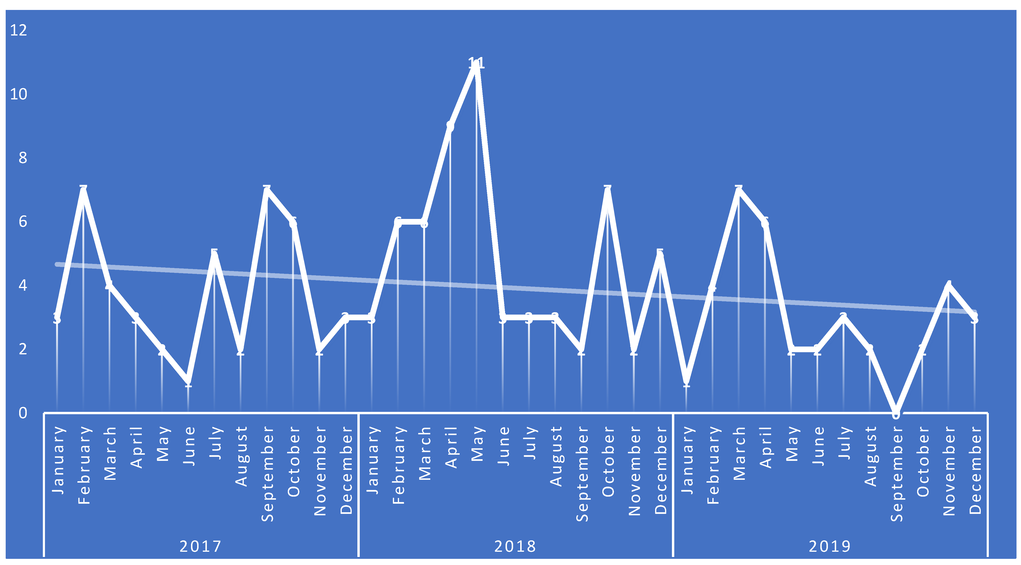
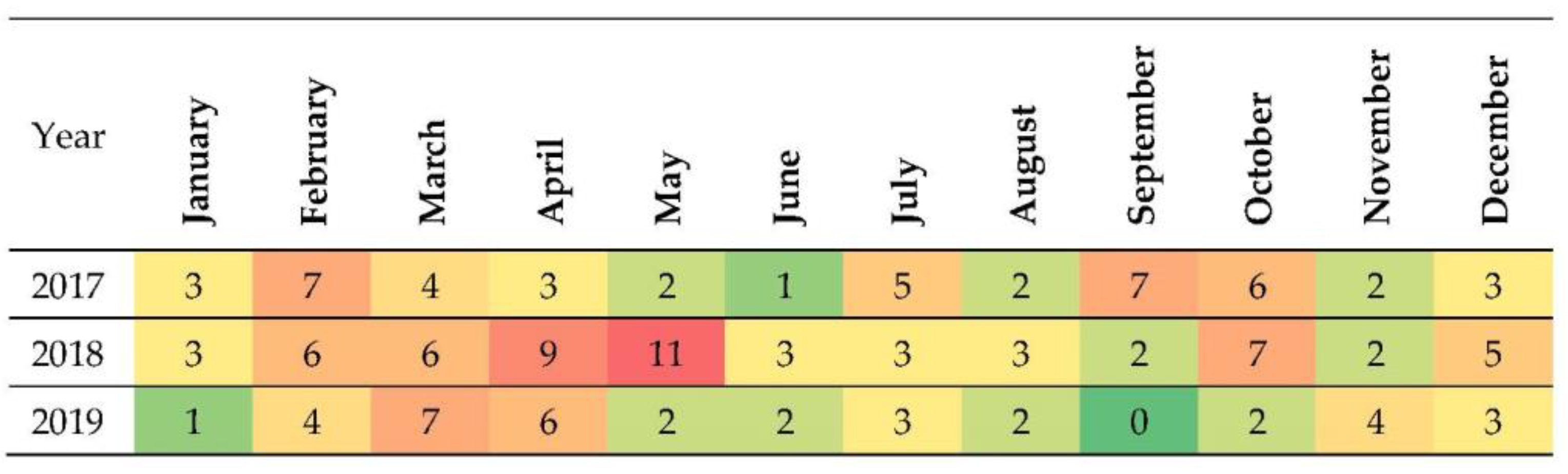
In order to analyze the seasonality of the data, we graphically represented the chronogram (Figure 1) and “heat map” (Figure 2) using Excel, for the analyzed period.

When modelling this component, it is necessary to determine to what extent and in what direction the seasonality of the time series terms deviates from the central tendency, in different phases of the period, usually of the year [41] (p. 215), since in the profile literature the seasonality is investigated after the elimination of the trend [42] (p. 233).

The seasonality index represents a relative issue that expresses the intensity of the seasonal wave that characterizes the evolution of the economic process in the annual sub period j (quarter, month) [43] (p. 207). The seasonality index results, in the case of the stationary series, are generated by relating the level of sub period j or the average of the values regarding sub period j for several years to the general average return for an annual sub period, according to the formula [43] (p. 207):

$$I_j^s=\frac{{{\displaystyle \sum }}_{i=1}^m\frac{y_{ij}}{m}}{\overline{y}}$$

(1)

where

$$\{\begin{array}{l}i=1,2,\dots m\mathrm{years}\\ j=1,2,\dots h\mathrm{quarters}/\mathrm{months}\\ \overline{y}=\mathrm{quarterly}/\mathrm{monthly}\mathrm{average}\mathrm{over}\mathrm{the}\mathrm{entire}\mathrm{interval}\end{array}$$

In the case of the trend series (non-stationary time series), it is recommended that, in a first phase, “to eliminate the trend can be achieved by relating the empirical (real) values y_i to the (adjusted) trend values Y_i and then calculating the indices of seasonality” using the formula [44] (p. 199). Therefore, [43] (p. 207):

$$I_j^s=\frac{\left[{{\displaystyle \sum }}_i\left(y_{ij}/Y_{ij}\right)\right]:m}{\left({{\displaystyle \sum }}_i{{\displaystyle \sum }}_j{y}_{ij}/Y_{ij}\right):mh}$$

(2)

where Y_ij = the central trend.

In the situation when $I_j^s$ > 1, the evolution from “season” j is higher than the average (peak season); if $I_j^s$ < 1, the evolution from “season” j is lower than the average (weak season).

To determine the seasonality indices, we used the multiplicative model. The specific stages are [41] (pp. 218–219):

(a) The ratio between the terms of the chronological series (y_ij) and the corresponding values of the trend (Y_ij), obtained by the method of moving averages or other trend analytical methods, is determined. The reports contain the seasonal component and the random component (ε_ij), according to the relation:

$$y_{ij}/Y_{ij}=S_j{}^{*}\cdot {\epsilon }_{ij}$$

where: i = 1, …, n; and j = 1, …, m.

(b) The partial means ($S_j{}^{*’}$) are calculated on sub periods with the help of the arithmetic mean, partial means called estimators of the seasonal component:

$$S_j{}^{*’}=\frac{1}{n}\left[{\displaystyle \sum \frac{y_{ij}}{Y_{ij}}}\right]=\frac{1}{n}{\displaystyle \sum \left(S_j{}^{*}\cdot {\epsilon }_{ij}\right)}=S_j{}^{*}\frac{{\displaystyle \sum {\epsilon }_{ij}}}{n}\cong S_j{}^{*}$$

(3)

If the trend was not calculated based on an analytical adjustment method, the product of the estimators $S_j{}^{*’}$ is different from 1 (Πs_j^*’ ≠ 1), we move on to the next step.

(c) The ratios between the estimators and their average are calculated, the calculation is for each sub period (season/month); thus, the corrected estimator of the seasonal component is obtained, also called seasonality index $S_j{}^{*}\left(I^S{}_j\right)$ of the sub period/month (season) “j” after the relationship:

$$S^{*}{}_j=S^{*’}{}_j:S^{*’}{}_j$$

(4)

meaning

$$S_j{}^{*}\left(I^S{}_j\right)=\left[\frac{1}{n}{\displaystyle \sum \frac{y_{ij}}{Y_{ij}}}\right]:\left(\frac{1}{m}{\displaystyle \sum S_j{}^{*’}}\right)=\frac{S^{*’}{}_j}{\frac{1}{m}\left({\displaystyle \sum S^{*’}{}_j}\right)}\cdot 100$$

(5)

The number of seasonality indices is equal to the number of sub periods (m).

The intensity of the seasonal wave is expressed by seasonality indices, determined according to the following formula, based on the method of reporting to the average [45] (p. 664):

$$I_j=\frac{{\overline{y}}_j}{\overline{y}}\cdot 100$$

(6)

The interpretation of seasonality indices is similar to that of the difference (Δ_j); in other words, an index greater than or equal to 100% corresponds to a peak period, and an index less than 100% is specific to a weak period.

Moreover, the linear function was used to calculate the trend for the pipeline incidents.

The principle of linear adjustment [46] (p. 169) is based on minimizing the vertical distances between the observed (empirical) values and the theoretical (adjusted) values provided by the adjustment line, also known as the method of smaller squares, respectively, $Min={{\displaystyle \sum }}^{\text{}}{\left(y_i-Y_i\right)}^2$ [41] (p. 209).

The linear trend is used if it is found that the graph shows an absolutely constant upward or downward trend, verified by a small variation of the absolute changes with the moving base [44] (p. 187), [41] (p. 209).

The linear model is based on the first degree function according to the relation:

$$Y_i=a+b*t_i$$

(7)

where a and b are the parameters of the function that are determined from the system of normal equations, obtained by the least squares method, as follows [45] (p. 637):

$$\{\begin{array}{c}a*n+b*{{\displaystyle \sum }}^{\text{}}{t}_i={{\displaystyle \sum }}^{\text{}}{y}_i\\ a*{{\displaystyle \sum }}^{\text{}}{t}_i+b*{{\displaystyle \sum }}^{\text{}}{t}_i^2={{\displaystyle \sum }}^{\text{}}{t}_i{y}_i\end{array}$$

(8)

and if the condition is set as ${{\displaystyle \sum }}^{\text{}}{t}_i$ = 0, the system (8) becomes:

$$\{\begin{array}{c}a*n={{\displaystyle \sum }}^{\text{}}{y}_i\\ b*{{\displaystyle \sum }}^{\text{}}{t}_i^2={{\displaystyle \sum }}^{\text{}}{t}_i{y}_i\end{array}$$

(9)

hence, the parameter $a=\frac{{{\displaystyle \sum }}^{\text{}}{y}_i}{n}$ and the parameter $b=\frac{{{\displaystyle \sum }}^{\text{}}{t}_i{y}_i}{{{\displaystyle \sum }}^{\text{}}{\mathrm{t}}_{\mathrm{i}}^2}$.

To analyze the data, descriptive statistics were used; the calculations were performed using SPSS 23.0 licensed (Statistical Package for Social Science), respectively: mean, standard deviation, minimum value, and maximum value.

To analyze whether there are differences between the mean values of each variable, the Kruskal–Wallis test was applied using SPSS 23.0 software. The Kruskal–Wallis test by ranks, Kruskal–Wallis H test (or one-way ANOVA on ranks) is a non-parametric method for testing whether samples originate from the same distribution. It is used for comparing two or more independent samples of equal or different sample sizes.

The Kruskal–Wallis test is a non-parametric test that takes into account not the absolute value of the observations but their rank, the calculation formula being the following:

$$K=12\times {\displaystyle \sum \left(T_j^2/n_j\right)/[N(N+1)]-3(N+1)}$$

(10)

where N = total number of observations;

T_j = total treatment modalities j.

Additionally, the calculation of the Pearson parametric correlation coefficient was taken into account. The calculation of the Pearson parametric correlation coefficient is based on the following formula:

$$R_{xy}=\frac{n{{\displaystyle \sum }}_{i=1}^n{x}_i{y}_i-\left({{\displaystyle \sum }}_{i=1}^n{x}_i\right)\left({{\displaystyle \sum }}_{i=1}^n{y}_i\right)}{\sqrt{\left[n{{\displaystyle \sum }}_{i=1}^n{x}_i^2-{\left({{\displaystyle \sum }}_{i=1}^n{x}_i\right)}^2\right]\left[n{{\displaystyle \sum }}_{i=1}^n{y}_i^2-{\left({{\displaystyle \sum }}_{i=1}^n{y}_i\right)}^2\right]}}$$

(11)

In order to test whether there are statistically significant differences of registered incidents depending on year of incident/incident type/product type/month/county/year of incident occurred, referring to the cause of the breakdown, the Chi-Square bivariate test was applied, the results being presented in structured tables in the Section 4. The SPSS 23.0 software was used to process data while the Chi-Square bivariate test used the following general hypothesis: H₀ = There are no statistically significant differences depending on year of incident/incident type/product type/month/county/year of incident occurred, referring to the cause of the breakdown.

In order to be able to verify this hypothesis, the following formula will be applied for the calculation of the statistics χ², statistics that will be calculated for a significance level of p-value α = 0.05.

$${\mathsf{\chi }}^2={\displaystyle \sum }_{i=1}^k[\frac{{\left(f_0-f_t\right)}^2}{f_t}]$$

(12)

where

$$\{\begin{array}{l}{f}_0=observedfrequencies\\ f_t=theoreticalfrequencies\end{array}$$

It is analyzed if the requirements of application of the test are met, respectively:

-

The sample has more than 50 statistical observations;

-

There are no cells with values less than 5 or equal to zero;

-

Values are absolute values and not percentages.

-

The decision to reject or accept the statistical hypothesis is as follows:

-

Comparing the two values (calculated with SPSS and the theoretical one, from the distribution tables); if it is observed that χ²_calculated < χ²_theoretical then it results in the null hypothesis H₀ being accepted and therefore there are no statistically significant differences;

-

Comparing the two values (calculated with SPSS and the theoretical one, from the distribution tables); if it is observed that χ²_calculated > χ²_theoretical then it results in the null hypothesis H₀ being rejected and therefore there are statistically significant differences.

For continuous variables from the study, the Student t test (independent) is used to analyze the statistically significant differences, and the results are presented in the last part of the next section.

4. Results

From Figure 1 it is observed that, regarding the number of incidents per month, in the analyzed period we can say that there is certainty regarding their seasonality; respectively, the peak season is the first quarter, more specifically for 2018 and 2019, March–April. The weak seasons are represented by the summer months, predominantly. For the analyzed period, the trend of the number of incidents/month was decreasing, as can be seen in Figure 1. Although the seasonality by quarters indicates the 2nd quarter as the peak season for all years, detailed by months, atypical aspects are observed, respectively, asymmetries within a quarter. For 2017, February is the peak season, while for 2018, the peak season is represented by May and for 2019 by March. Another atypical situation is shown by the fact that, for the years 2017 and 2018, September is also the peak season, while for 2019, in September, no incidents were registered. A symmetry that must be signaled is shown by the fact that, in each of the 3 years, June represents the weak season.

We made, for the same indicator, Number of incidents per month, and a graph type “heat map” (Figure 2), the data being monthly in order to better see the months of the year with the highest number of such events. The figure contains values on green background (reduced number of breakdowns per month) and values on red background (increased number of incidents per month).

It can be seen that the large number of events is concentrated in spring and September–October with a maximum in 2018 in April and May.

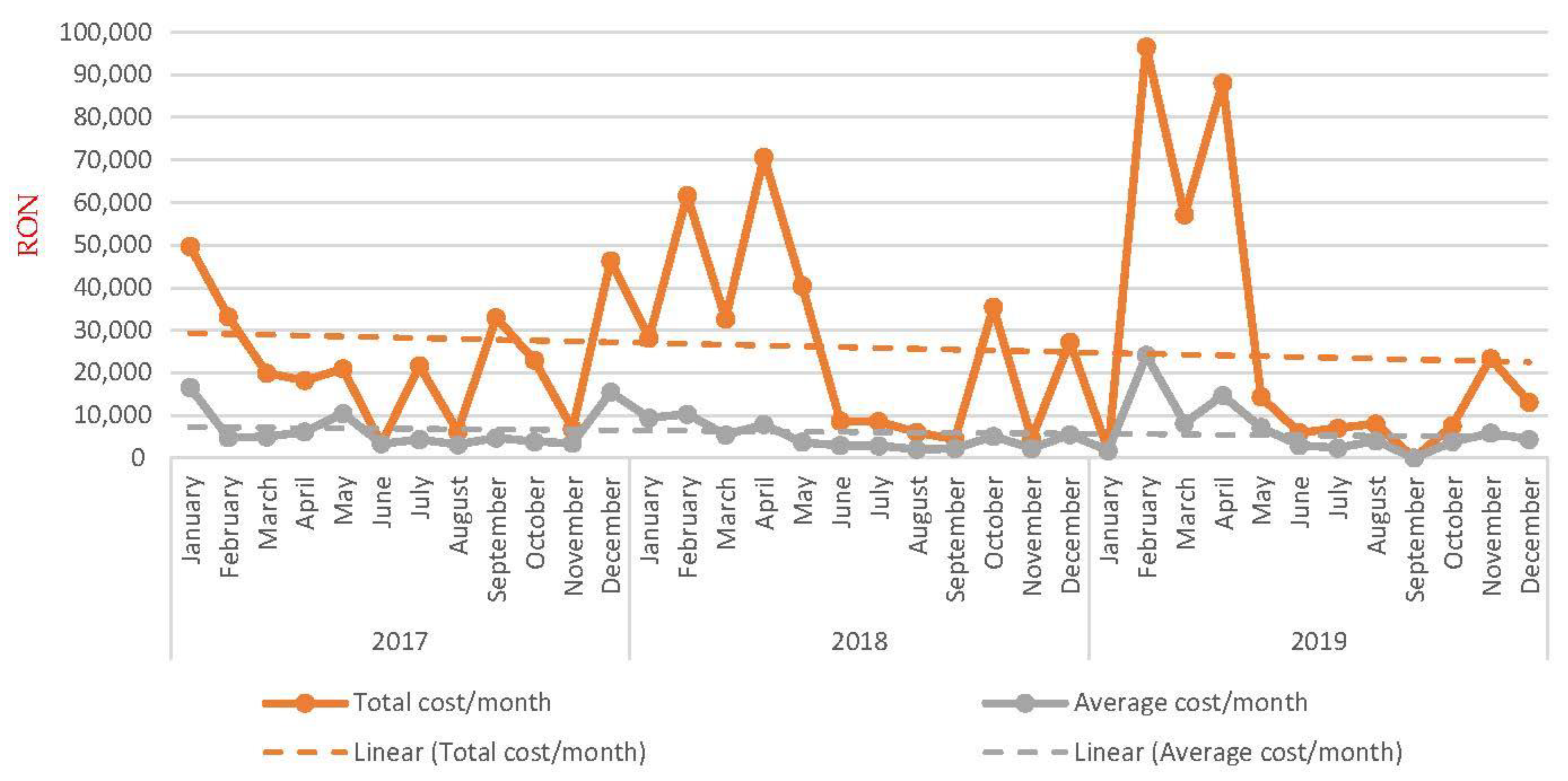
Figure 3 shows the time series (chronogram) for the variables total cost per month and average cost per month. From Figure 3 it can be seen that, for the analyzed period, both variables had a decreasing trend. The values from Y axis refer to the local currency (1 USD = 4.2 RON).

Table 2. Descriptive statistics and p-value for number of incidents, total cost/month, and average cost/month.

	2017	2018	2019	p-Value *
Total number of incidents/month	4 ± 2 (1–7)	5 ± 3 (2–11)	3 ± 2 (0–7)	0.182
Total cost/month (RON)	23,525.75 ± 14,843.16 (3331.05–49,662.80)	27,361.56 ± 22,425.64 (4405.09–70,687.77)	26,897.18 ± 34,105.78 (0–96,548.27)	0.710
Average cost/month (RON)	6751.52 ± 4747.47 (3114.22–16,554.27)	4942.23 ± 2877.15 (1996.36–10,278.50)	6595.06 ± 6706.59 (0–24,137.07)	0.567

* p-value was calculated with the Kruskal–Wallis test.

presents descriptive statistics for the variables number of incidents, total cost/month, and average cost/month. Data are presented as: mean ± std. Deviation (minimum–maximum). To analyze whether there are differences between the mean values of each variable in column 1, the Kruskal–Wallis test was applied using SPSS software.

Since the p-values of the level are not statistically significant, based on the Kruskal–Wallis test they are over 0.05, there are no statistically significant differences between the average values of these indicators, depending on the year in which they were recorded (

Table 3. Results for Kruskal–Wallis Test ^a,b.

	Total Number of Incidents/Month	Total Cost/Month	Average Cost/Month
Chi-Square	3.405	0.686	1.135
df	2	2	2
Asymp. Sig.	0.182	0.710	0.567

^a Kruskal–Wallis test; ^b grouping variable: year of incident registration.

).

Thus, the normality of the distribution of these indicators was further tested using the One-Sample Kolmogorov–Smirnov test; the p-value < 0.05 for all three indicators, so all of them had a normal distribution (

Table 4. Results for normal distribution test with One-Sample Kolmogorov–Smirnov Test.

		Total Number of Incidents/Month	Total Cost/Month (RON)	Average Cost/Month (RON)
N		36	36	36
Normal Parameters a,b	Mean	3.92	25,928.1658	6096.2682
	Std. Deviation	2.430	24,410.74107	4950.79784
Most Extreme Differences	Absolute	0.230	0.153	0.224
	Positive	0.230	0.153	0.224
	Negative	−0.132	−0.144	−0.160
Test Statistic		0.230	0.153	0.224
Asymp. Sig. (2-tailed)		0.000 c	0.033 c	0.000 c

^a Test distribution is normal; ^b calculated from data; ^c Lilliefors significance correction.

).

It was tested if there are statistically significant correlations between the three indicators, the results being presented in

Table 5. Pearson Correlation coefficients.

		Total Incidents/Month	Total Cost/Month	Average Cost/Month
Total number of incidents/month	Pearson Correlation	1	0.622 **	0.175
	Sig. (2-tailed)		0.000	0.306
	N	36	36	36
Total cost/month	Pearson Correlation		1	0.827 **
	Sig. (2-tailed)			0.000
	N		36	36
Average cost/month	Pearson Correlation			1
	Sig. (2-tailed)
	N			36

**. Correlation is significant at the 0.01 level (2-tailed).

. Thus, there is a direct (positive) correlation of medium to strong intensity (0.622) that is statistically significant (p-value = 0.000) between the total number of incidents per month and the total cost. Moreover, Table 5 presents the results obtained with SPSS software (in fact x and y in the Formula (11) take the values of each pair in turn, for example: total number of incidents per month and total costs per month, etc.).

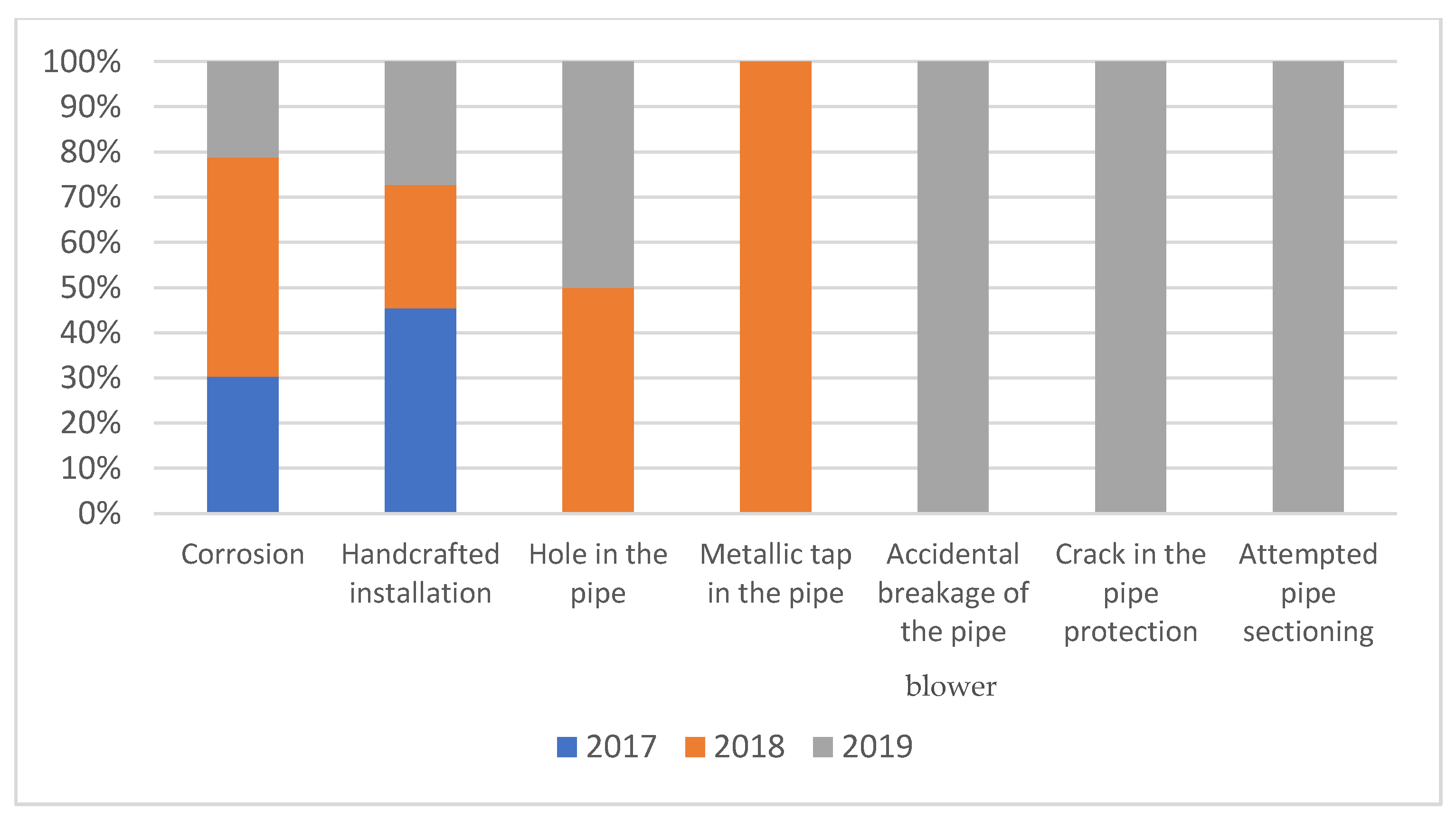
The following table is related to the cross-tabulation (

Table 6. The cross-tab for cause and year of incident registration.

	Year of Incidence	2017	2018	2019	Total
Cause
Corrosion		30	48	21	99
Handcrafted installation		15	9	9	33
Hole in the pipe		0	1	1	2
Metallic tap in the pipe		0	1	0	1
Accidental breakage of the pipe blower		0	0	2	2
Crack in pipe protection		0	0	1	1
Attempted pipe sectioning		0	0	2	2
Total		45	59	36	140

) and summarizes the causes of incidents for each year and also this info is represented graphically in Figure 4.

For the total analyzed period, the distribution of the incident causes is in the following table (

Table 7. Hierarchy of incident causes for 2017–2019.

	Frequency	Percent	Valid Percent	Cumulative Percent
Corrosion	99	70.2	70.7	70.7
Handcrafted installation	33	23.4	23.6	94.3
Hole in the pipe	2	1.4	1.4	95.7
Metallic tap in the pipe	1	0.7	0.7	96.4
Accidental breakage of the pipe blower	2	1.4	1.4	97.9
Crack in pipe protection	1	0.7	0.7	98.6
Attempted pipe sectioning	2	1.4	1.4	100.0
Total	140	99.3	100.0
Missing system	1	0.7
Total	141	100.0

), the most common being corrosion—70.2% and handcrafted installation—23.4% of the total causes.

According to the analysis of the recorded incidents, in the table below the absolute and relative frequencies of where the incidents occurred were calculated, and most of the events took place at the following pipes, marked in red in the table (

Table 8. Recorded incidents by pipe localization and type.

	Frequency	Percent	Valid Percent	Cumulative Percent
Ø 10 3/4” Icoana-Cartojani	4	2.8	2.8	2.8
Ø 10 3/4” Madulari-Botorani	1	0.7	0.7	3.5
Ø 10 3/4” Vermesti-Tg. Ocna	1	0.7	0.7	4.3
Ø 10 3/4” F1 Bărbătești-Orleș	2	1.4	1.4	5.7
Ø 10 3/4” F1 Barbatesti-Orlesti	1	0.7	0.7	6.4
Ø 10 3/4” F1 Orlesti-P. Lacului	1	0.7	0.7	7.1
Ø 10 3/4” F1 Orlesti-Poiana Lacul	1	0.7	0.7	7.8
Ø 10 3/4” F1 P. Lacului-Siliste	1	0.7	0.7	8.5
Ø 10 3/4” F2 Orlesti-P. Lacului	1	0.7	0.7	9.2
Ø 10 3/4” F2 Orlesti-Poiana Lacul	2	1.4	1.4	10.6
Ø 10 3/4” F2 Poiana Lacului-Silis	1	0.7	0.7	11.3
Ø 10 3/4” F2 Rădinești-Orlești	1	0.7	0.7	12.1
Ø 10 3/4” F2 Siliste-Ploiesti	3	2.1	2.1	14.2
Ø 10 3/4” Icoana-Cartojani	2	1.4	1.4	15.6
Ø 10” Centura	1	0.7	0.7	16.3
Ø 10” F1 Barbatesti-Ploiesti	1	0.7	0.7	17.0
Ø 10” Ghercesti-Icoana	1	0.7	0.7	17.7
Ø 10” Icoana-Cartojani	1	0.7	0.7	18.4
Ø 10” Poiana Lacului-Siliste F1	1	0.7	0.7	19.1
Ø 10” Lascar C.-Independenta	1	0.7	0.7	19.9
Ø 12 3/4” Cartojani-Ploiesti	3	2.1	2.1	22.0
Ø 12” Cartojani-Ploiesti	1	0.7	0.7	22.7
Ø 12” F1 Calareti-Ploiesti	1	0.7	0.7	23.4
Ø 14 3/4” Brazi Refinery	1	0.7	0.7	24.1
Ø 14 3/4” Cartojani-Ploiesti	2	1.4	1.4	25.5
Ø 14” Calareti-Pitesti	2	1.4	1.4	27.0
Ø 14” Constanta-Arpechim	2	1.4	1.4	28.4
Ø 14” Constanta-Baraganu	1	0.7	0.7	29.1
Ø 20” Baraganu-Calareti	2	1.4	1.4	31.2
Ø 20” Baraganu-Călăreți	1	0.7	0.7	29.8
Ø 20” Călăreți-Pitești	1	0.7	0.7	31.9
Ø 20” Constanta-Baraganu	16	11.3	11.3	43.3
Ø 24” Baraganu-Calareti	15	10.6	10.6	53.9
Ø 24” Calareti-Pietrosani	2	1.4	1.4	55.3
Ø 24” Calareti-Ploiesti	7	5.0	5.0	60.3
Ø 24” Constanta-Petromidia	3	2.1	2.1	62.4
Ø 28” Constanta-Baraganu	5	3.5	3.5	66.0
Ø 4 + 5” Surani-Matita	1	0.7	0.7	66.7
Ø 4” Recea-Mislea	1	0.7	0.7	67.4
Ø 4”+ 5” Surani-Magurele	2	1.4	1.4	68.8
Ø 4”+ 5” Surani-Matita	2	1.4	1.4	70.2
Ø 5 9/16” G. Vitioarei-Ploiesti	2	1.4	1.4	71.6
Ø 5 9/16” Gura Vit.-Magurele	1	0.7	0.7	72.3
Ø 5 9/16” Păcureți-Măgurele	1	0.7	0.7	73.0
Ø 5” GuraVitioarei-Boldești	1	0.7	0.7	73.8
Ø 6 + 5” GuraVitioarei-Boldeșt	1	0.7	0.7	74.5
Ø 6 5/8” Baicoi-Banesti	1	0.7	0.7	75.2
Ø 6 5/8” F1 Ticleni-Ploiesti	5	3.5	3.5	78.7
Ø 6 5/8” Grindu-Urziceni	2	1.4	1.4	80.1
Ø 6 5/8” Izvoru-Izvoruracordare	2	1.4	1.4	81.6
Ø 6 5/8” Moreni-Ploiesti	1	0.7	0.7	82.3
Ø 6 5/8” Ochiuri-Moreni	1	0.7	0.7	83.0
Ø 6 5/8” Padure II-Buda	2	1.4	1.4	84.4
Ø 6 5/8” Teis-Moreni	3	2.1	2.1	86.5
Ø 6 5/8” Urlati-Ploiesti	3	2.1	2.1	88.7
Ø 6 5/8” Urziceni-Albesti	6	4.3	4.3	92.9
Ø 6 5/8” Urziceni-Ploiesti	2	1.4	1.4	94.3
Ø 6 5/8” Lact-Icoana	1	0.7	0.7	95.0
Ø 6” Izvoru-Izvoruracordare	1	0.7	0.7	95.7
Ø 8” Lucacesti-Vermesti	1	0.7	0.7	96.5
Ø 8 + 6”Oprisenesti-Ciresu	1	0.7	0.7	97.2
Ø 8 5/8” Boldesti-Raf Teleajen	1	0.7	0.7	97.9
Ø 8 5/8” Centura	1	0.7	0.7	98.6
Ø 8” Lucacesti-Vermesti	1	0.7	0.7	100.0
Ø 8” Lucăcești-Vermești	1	0.7	0.7	99.3
Total	141	100.0	100.0

).

The table below includes the counties with the highest number of pipe incidents in the analyzed period, marked in red in the table (

Table 9. Recorded incidents by county.

	Frequency	Percent	Valid Percent	Cumulative Percent
Ialomita	10	7.1	7.1	7.1
Valcea	6	4.3	4.3	11.3
Arges	15	10.6	10.6	22.0
Calarasi	19	13.5	13.5	35.5
Prahova	32	22.7	22.7	58.2
Ilfov	4	2.8	2.8	61.0
Dambovita	17	12.1	12.1	73.0
Constanta	23	16.3	16.3	89.4
Bacau	4	2.8	2.8	92.2
Teleorman	2	1.4	1.4	93.6
Gorj	3	2.1	2.1	95.7
Giurgiu	3	2.1	2.1	97.9
Galati	1	0.7	0.7	98.6
Olt	1	0.7	0.7	99.3
Braila	1	0.7	0.7	100.0
Total	141	100.0	100.0

).

Among the transported oil products, the product most affected by the incidents was domestic crude oil (55.3%), followed by imported crude oil product with 41.1% (

Table 10. Recorded incidents by transported product.

	Frequency	Percent	Valid Percent	Cumulative Percent
Crude oil (from Romania)	78	55.3	55.3	55.3
Imported crude oil	58	41.1	41.1	96.5
Gasoline	5	3.5	3.5	100.0
Total	141	100.0	100.0

).

The most common incident is the technical one with 73% of the total, the difference being represented by the intentionally caused incident, with 27% of the total (

Table 11. Recorded incidents by incident type.

	Frequency	Percent	Valid Percent	Cumulative Percent
Technical	103	73.0	73.0	73.0
Intentionally caused	38	27.0	27.0	100.0
Total	141	100.0	100.0

).

It is worth highlighting the high frequency of “intentionally caused” incidents. The fact that petroleum products (representing important and expensive conventional resources) are transported on these pipelines, which, through excise duty, are sold at significantly higher price values, explains the temptation to use artisanal installations through which to divert substantial quantities. This situation reveals the continuous concern of the decision makers in proposing ample measures and actions for monitoring on the ground and in the air, through which to prevent such incidents/provoked breakdowns.

In order to perform the Chi-Square test, cross-tabulation is used again. Cross-tabulation greatly helps in research by identifying patterns, trends, and the correlation between parameters. Therefore, a cross-tabulation is made regarding the year of incident registration and causes of incident for each analyzed year.

Table 12. The cross-tab for year of incident registration and cause of incident.

	Cause	Corrosion	Handcrafted Installation	Hole in the Pipe	Metallic Tap in the Pipe	Accidental Breakage of the Pipe blower	Crack in Pipe Protection	Attempted Pipe Sectioning	Total
Year of Incident Registration
2017		30	15	0	0	0	0	0	45
2018		48	9	1	1	0	0	0	59
2019		21	9	1	0	2	1	2	36
Total		99	33	2	1	2	1	2	140

was built based on it.

The defining results of the Chi-Square test can be found in

Table 13. Results for Chi-Square bivariate test.

	Value	df	Asymptotic Sig. (2-Sided)
Pearson Chi-Square	22.360	12	0.034
Likelihood Ratio	22.440	12	0.033
Linear-by-Linear Association	7.363	1	0.007
N of Valid Cases	140

.

From Table 13, because the p-value is <0.05, the null hypothesis H₀ is rejected and therefore there are significant differences depending on the cause of the incident related to the year in which the incident occurred (one of the observable differences in Table 12—cross-tab being the much higher number of incidents in 2016 caused by handcrafted installations).

Another cross-tabulation concerns the incident type–incident cause pair. The cross-tabulation results are mentioned in

Table 14. The crosstab for incident type and cause.

	Cause	Corrosion	Handcrafted Installation	Hole in the Pipe	Metallic Tap in the Pipe	Accidental Breakage of the Pipe Blower	Crack in Pipe Protection	Attempted Pipe Sectioning	Total
Incident Type
Technical		99	0	0	0	2	1	0	102
Intentionally caused		0	33	2	1	0	0	2	38
Total		99	33	2	1	2	1	2	140

.

Table 15. The results for Chi-Square bivariate test.

	Value	df	Asymptotic Sig. (2-Sided)
Pearson Chi-Square	140.000	6	0.000
Likelihood Ratio	163.709	6	0.000
Linear-by-Linear Association	39.822	1	0.000
N of Valid Cases	140

contains the Chi-Square test, and in this case it is observed that the null hypothesis H₀ is rejected (p-value = 0.000) and therefore there are statistically significant differences depending on the cause of the pipe incident and the incident type for the analyzed period.

Another pair of elements refers to the type of product transported through the pipeline and the incident cause. The cross-tabulation results are included in

Table 16. The cross-tab for product type and cause.

	Cause	Corrosion	Handcrafted Installation	Hole in the Pipe	Metallic Tap in the Pipe	Accidental Breakage of the Pipe Blower	Crack in Pipe Protection	Attempted Pipe Sectioning	Total
Product Type
Crude oil (from Romania)		53	20	0	0	2	1	2	78
Imported crude oil		41	13	2	1	0	0	0	57
Gasoline		5	0	0	0	0	0	0	5
Total		99	33	2	1	2	1	2	140

.

Thus,

Table 17. The results for Chi-Square bivariate test.

	Value	df	Asymptotic Sig. (2-Sided)
Pearson Chi-Square	10.380	12	0.583
Likelihood Ratio	14.384	12	0.277
Linear-by-Linear Association	2.564	1	0.109
N of Valid Cases	140

describes the corresponding Chi-Square test.

The conclusion is that regarding the cause of the pipe incident and the type of product, the results indicate that there are no statistically significant differences.

Moreover, there are no differences depending on the cause and the month of the year when the incident occurred, according to the results of the Chi-Square test in the table below (

Table 18. The results for Chi-Square bivariate test.

	Value	df	Asymptotic Sig. (2-Sided)
Pearson Chi-Square	65.515	66	0.494
Likelihood Ratio	49.988	66	0.929
Linear-by-Linear Association	0.866	1	0.352
N of Valid Cases	140

).

In addition, there are no differences depending on the cause and the county in which the incident occurred, according to the results of the Chi-Square test in the table below (

Table 19. The results for Chi-Square bivariate test.

	Value	df	Asymptotic Sig. (2-Sided)
Pearson Chi-Square	89.482	84	0.321
Likelihood Ratio	62.467	84	0.962
Linear-by-Linear Association	0.309	1	0.579
N of Valid Cases	140

).

Last but not least, there are no differences depending on the cause and the year in which the incident occurred, according to the results of the Chi-Square test in the table below (

Table 20. The results for Chi-Square bivariate test.

	Value	df	Asymptotic Sig. (2-Sided)
Pearson Chi-Square	840.000	834	0.435
Likelihood Ratio	234.739	834	1.000
Linear-by-Linear Association	2.497	1	0.114
N of Valid Cases	140

).

To analyze whether there are statistically significant differences depending on the type of incident between the average values of the other indicators in the study, the Student’s t test was applied, the results being presented in the following tables (

Table 21. Descriptive statistics of Student’s t test.

	Incident Type	N	Mean	Std. Deviation	Std. Error Mean
Cause	Technical	102	1.13	0.740	0.073
	Intentionally caused	38	2.37	1.172	0.190
Cost	Technical	103	7344.4314	11,934.05523	1175.89740
	Intentionally caused	38	4656.2511	3531.61935	572.90431
Incident data	Technical	103	30 May 2018	276.07:22:36.543	27.05:24:32.304
	Intentionally caused	38	15 May 2018	326.05:09:54.642	52.22:03:29.885
County	Technical	103	5.42	2.721	0.268
	Intentionally caused	38	6.29	3.075	0.499
Month	Technical	103	6.17	3.552	0.350
	Intentionally caused	38	5.87	3.086	0.501
Transported product	Technical	103	1.50	0.592	0.058
	Intentionally caused	38	1.42	0.500	0.081

and

Table 22. Results for Student’s t test.

		Levene’s Test for Equality of Variances		t-Test for Equality of Means
		F	Sig.	t	df	Sig. (2-Tailed)	Mean Difference	Std. Error Difference	95% Confidence Interval of the Difference
									Lower	Upper
Cause	Equal variances assumed	6.975	0.009	−7.444	138	0.000	−1.241	0.167	−1.571	−0.911
	Equal variances not assumed			−6.089	48.419	0.000	−1.241	0.204	−1.651	−0.831
Cost	Equal variances assumed	4.413	0.037	1.364	139	0.175	2688.18	1970.92749	−1208.69361	6585.05423
	Equal variances not assumed			2.055	135.174	0.042	2688.18	1308.03442	101.32089	5275.03973
Incident type	Equal variances assumed	5.628	0.019	0.271	139	0.787	14.22:52:18.27	55.02:58:48.902	−94.00:53:43.219	123.22:38:19.765
	Equal variances not assumed			0.251	57.712	0.803	14.22:52:18.27	59.12:16:57.600	−104.04:27:02.096	134.02:11:38.642
County	Equal variances assumed	0.462	0.498	−1.630	139	0.105	−0.872	0.535	−1.930	0.186
	Equal variances not assumed			−1.540	59.657	0.129	−0.872	0.566	−2.005	0.261
Month	Equal variances assumed	1.964	0.163	0.470	139	0.639	0.306	0.652	−0.982	1.595
	Equal variances not assumed			0.502	75.469	0.617	0.306	0.611	−0.910	1.523
Transported product	Equal variances assumed	2.949	0.088	0.776	139	0.439	0.084	0.108	−0.130	0.297
	Equal variances not assumed			0.838	77.581	0.404	0.084	0.100	−0.115	0.283

).

The above results show that, if we group the study data according to the type of incident, there are statistically significant differences between the averages of the following variables in the study: cause of incident, total cost of incident, and incident type (p-value < 0.05), and for the transported product, a level of statistical significance of 91.2%.

Table 23. Pearson correlation coefficients.

		Cause	Cost	County	Month	Product	Incident Type
Cause	Pearson Correlation	1	0.134	0.047	−0.079	−0.136	0.535 **
	Sig. (2-tailed)		0.114	0.580	0.354	0.110	0.000
	N	140	140	140	140	140	140
Cost	Pearson Correlation		1	−0.075	−0.172 *	−0.006	−0.115
	Sig. (2-tailed)			0.380	0.041	0.945	0.175
	N		141	141	141	141	141
County	Pearson Correlation			1	0.110	0.069	0.137
	Sig. (2-tailed)				0.194	0.414	0.105
	N			141	141	141	141
Month	Pearson Correlation				1	0.105	−0.040
	Sig. (2-tailed)					0.213	0.639
	N				141	141	141
Product	Pearson Correlation					1	−0.066
	Sig. (2-tailed)						0.439
	N					141	141
Incident type	Pearson Correlation						1
	Sig. (2-tailed)
	N						141

** Correlation is significant at the 0.01 level (2-tailed). * Correlation is significant at the 0.05 level (2-tailed).

contains the matrix of Pearson parametric correlation coefficients.

The following statistically significant correlations are the result:

-

There is a statistically significant direct correlation of average intensity (Pearson correlation coefficient = 0.535) between the type of incident and its cause;

-

There is a statistically significant inverse correlation of low intensity (Pearson correlation coefficient = −0.172) between the month of incident and its cost.

5. Conclusions

This paper presents a statistical analysis of the main oil pipeline system from Romania in terms of failure event rates and the hierarchy of the main causes of incidents.

The causes identified and analyzed were classified into seven categories: corrosion; handcrafted (artisanal) installation; hole in the pipe; metallic tap in the pipe; accidental breakage of the pipe blower; crack in pipe’s protection; attempted pipe sectioning.

Major pipeline incident events often result in injuries, fatalities, property damage, fires, explosions, and release of hazardous materials. Because of these multiple consequences, detailed statistical analyses are needed related to the causes that generated these events.

In this sense, any analysis has to start from the following description regarding the general condition of the oil and gas transport systems: it is known that most European pipeline systems were built in the 1960s and 1970s, while in 2019 less than 2% of the pipelines were 10 years old or less and 70% were over 40 years old, and 40% of the pipeline networks worldwide have reached their projected 20-year service lifetime. This situation is similar in North America, Russia, and even Australia.

Over time, general and specific studies have been conducted on the analysis of incidents in oil and gas pipelines around the world. The most important studies were conducted in the United States (via PHMSA) and in Europe (by UKOPA and EGIG). The present study introduces representative elements in the case of incidents occurring in the national transport system of petroleum products in Romania in order to initiate useful steps in harmonizing the causes of these incidents with the analysis and recommendations of international professional associations in this field.

The main ideas and findings of the present analysis can be presented as follows:

-

The most common causes refer to corrosion (especially internal corrosion) and handcrafted (artisanal) installations (in this last case, the decision makers are inclined to intervene promptly by promoting ground and air patrol missions);

-

There is a linear tendency to reduce incidents due to artisanal installations (starting with 2017 when monitoring was started by patrolling crews with people, for land security and day by day checks);

-

Most incidents occurred in pipes with large diameters and while transporting imported crude oil;

-

The counties most affected by the incidents are represented by points of major interest (Constanta, with the crude oil terminal that ensures the supply of refineries with imported crude oil transported by vessels; Prahova, through the Brazi refinery that processes both crude and imported crude oil; Calarasi and Ialomita, as nodal points that have pumping stations for the transport of crude oil to Moldova and Muntenia);

-

There is a seasonality that shows that the 2nd quarter of each year (especially the months of March and April) presents an increased number of events; the explanation is given by the fact that these months are marked by numerous days with precipitation, and the patrol missions are hampered by the climatic conditions so that the incidents that have as a source the artisanal installations are more numerous; we meet the same situation in September.

-

There is a seasonality that shows up as well in the 2nd quarter of 2018 and 2019 (especially the months of February and April) for total cost per month and average cost per month due to the highest number of incidents in April and May 2018 (9, respectively, 11) from the entire analyzed period (according to the heat map from Figure 2);

-

Based on the results of the Kruskal–Wallis test, there are no differences between the studied years depending on number of incidents, total cost/month, and average cost/month;

-

There is positive statistical significance and medium through strong correlation between total cost/month and total number of incidents/month;

-

There is positive statistical significance and strong correlation between average cost/month and total cost/month;

-

According to the results of the Chi-Square bivariate test:

• There are statistically significant differences between the years from the study depending on the cause of incident and incident type;
• There are no statistically significant differences between the years from the study depending on product type, month in which incident occurred, county in which the incident occurred, cause of incident.

-

According to the results of Student’s t test, there are statistically significant differences depending on incident type between: the means of incident causes, the means of total cost, and the means of incident data;

-

There is positive statistical significance and medium correlation between incident type and incident cause;

-

There is negative statistical significance and weak correlation between the month of the incident and the total cost.

Taking into account these observations and the fact that crude oil is considered to be the “black” gold for a country’s economy, some measures have already been initiated, to which the authors add proposals to generate a more efficient use of crude oil resources (especially) using pipeline network. This more efficient use takes into account, on the one hand, natural economic requirements (cost of interventions, costs of replacing equipment and pipelines affected by accidents, monitoring costs, and costs of reducing or eliminating adverse effects on soil and water), and on the other hand, the creation of a much safer technical infrastructure to ensure the protection of the environment.

The concept targeted in the paper, including through statistical analysis, but also from the need to implement safe practices in order to prevent, detect, and mitigate incidents that may occur in the case of pipelines, refers to pipeline integrity. This approach chronologically includes the stages of prevention, detection, and mitigation. Each of these steps can significantly help reduce the negative financial, social, and environmental effects that any incident in this sector can generate at any given time.

Specifically, prevention involves: avoiding geo-hazards along pipelines; adequately protecting pipelines against corrosion; monitoring operating pressures; inspection of pipelines; and properly training all the operators and workers involved in the process.

Practically, detection deals with: external detection systems comprising sensors, imaging (with cameras, using drones and maybe helicopters), and patrols (with cars, helicopters, and drones); internal detection systems that check the commodity pressure and/or flow in the pipes, statistical analyses regarding the condition of the pipes made automatically by specialized interfaces. Mitigation aims to locate the area where there are spills, recover, by which quick measures are taken (maximum 6–8 h) to eliminate the effects generated by incidents, and, respectively, clean up, which refers to the cleaning of the place where commodity leaks have occurred.

Therefore, on the one hand, it is necessary to consider the continuation and development of the modernization programs initiated as follows: upgrading the hardware and software of the existing SCADA system (type MicroSCADA 8.4.3, produced and installed by ABB ENERGY INFORMATION SYSTEMS GMBH Germany, consisting of five Base System 1 and 2 servers-redundant, Frontend 1- and 2-redundant, and a remote access server); modernization of the cathodic protection system of the pipelines (currently consisting of a number of 218 cathodic protection stations—not integrated in a unitary automated system—located on the route of the main and local pipelines, respectively); implementation, for the first time, of a leak detection and location system (leak detection type); intelligent excavation of the pipeline system, respectively, through reconstruction by guided drilling (horizontal), of some important route segments, from the category of works of art (as is the case of crossing watercourses, as the currently established solution over crossing perpetually raises issues of the order of securing the supporting elements).

On the other hand, it is necessary to carry out concrete measures for strategic lines of action:

• Improvements of the national transport system by the implementation of the leak detection and location system, modernization of the cathodic protection system and supervisory, control, and data acquisition system (by developing existing SCADA system), and renewal of the pipeline network based on field data monitoring;
• Economic efficiency improvements by reduction of technological consumption within the storage and transport processes, minimization of energy, fuel, and lubricant consumptions, and reduction of the operating costs;
• Interconnection of the national crude oil pipeline transport system to the Regional and European Systems based on the implementation of Constanţa–Piteşti–Pancevo Project—an alternative crude oil transport solution in order to supply the Pancevo refinery (Serbia). This project has the following features:

  -

  Total length of the pipe—760 km;

  -

  Transport capacity—7.5 million tons/year;

  -

  Only the section pipe Pitești–Naidaș–Pancevo (440 km) needs to be built; the section pipe Constanta–Pitesti (320 km) is already built. Constanta is the main oil supply hub (for imported crude oil) in Eastern Europe and the Balkan countries.

• To comply with legal requirements applicable to the organization and to ensure a working environment in safe conditions, organizational, administrative, and financial efforts have to be continued to recertify the management systems already functional in the company (ISO 9001:2015; ISO 14001: 2015; ISO 45001:2018; ISO 50001:2018). Based on these recertified systems (last time in 2019), the inclusion of new procedures and the updating of existing ones regarding the inspection and maintenance plans of the pipeline systems must be considered.