Defect Detection on a Wind Turbine Blade Based on Digital Image Processing

Abstract

Wind power generation is a widely used power generation technology. Among these, the wind turbine blade is an important part of a wind turbine. If the wind turbine blade is damaged, it will cause serious consequences. The traditional methods of defect detection for wind turbine blades are mainly manual detection and acoustic nondestructive detection, which are unsafe and time-consuming, and have low accuracy. In order to detect the defects on wind turbine blades more safely, conveniently, and accurately, this paper studied a defect detection method for wind turbine blades based on digital image processing. Because the log-Gabor filter used needed to extract features through multiple filter templates, the number of output images was large. Firstly, this paper used the Lévy flight strategy to improve the PSO algorithm to create the LPSO algorithm. The improved LPSO algorithm could successfully solve the PSO algorithm’s problem of falling into the local optimal solution. Then, the LPSO algorithm and log-Gabor filter were used to generate an adaptive filter, which could directly output the optimal results in multiple feature extraction images. Finally, a classifier based on HOG + SVM was used to identify and classify the defect types. The method extracted and identified the scratch-type, crack-type, sand-hole-type, and spot-type defects, and the recognition rate was more than 92%.

1. Introduction

With the rapid development of the social economy and science and technology, people’s demand for the development of new energy is becoming more and more urgent [1]. Wind energy is a type of clean renewable energy that has advantages such as a relatively low difficulty of development and a small impact on the environment. It is understood that China’s installed wind power capacity jumped from 2007 until recently. Due to the increasing installed capacity, China has become one of the most important wind power countries in the world [2].

The blades of a wind turbine are a crucial component that determine whether the turbine can capture the wind efficiently and safely. Due to the impact of the working environment, the blades used by wind turbines require high strength, hardness, low density, and as long a service life as possible. Although great efforts have been made in the study of blade materials, various defects may occur during transportation, work, and installation, in the previously used wood blades to fiberglass blades, composite blades, and even the most advanced new composite blades [3]. The failure of blades will not only bring economic losses to wind power enterprises, but also cause serious safety problems. Therefore, timely and efficient detection of blade defects of wind turbines is particularly important.

Traditional defect-detection methods include percussion detection, telescope observation, and visual detection by sending people to high places to inspect the blades [4]. However, there are many kinds of defects, such as the sand-hole type, scratch type, crack type, and spot type. When judging these types, the accuracy of the above methods is often low, the process is time-consuming, and the manual-detection method has an especially high risk. These methods have to subjective factors, and the results are likely to be inaccurate [5]. Therefore, the purpose of this paper is to study a defect-detection method based on digital image processing. This method is simple and efficient, with higher accuracy and less risk than the traditional methods.

At present, the most widely used and direct method is the visual measurement method through manual detection [6]. We mainly observed the obvious defects such as scratches, sand hole, cracks and corrosion on the blade’s surface, as well as in its interior and on other areas [7], as shown in Figure 1.

With the development of new technology, acoustic-based nondestructive testing methods have been developed. Acoustic nondestructive testing (NDT) is a commonly used technology in wind turbine blade quality control worldwide, and includes the acoustic vibration method, ultrasonic echo method, laser ultrasonic method, and acoustic emission technology [8]. Among these, the ultrasonic echo method is the most widely used and has many advantages, such as a simple principle, convenient operation, low cost, strong penetration ability, and high sensitivity [9].

In recent years, with the continuous development of machine vision, using a machine-vision detection method is increasingly applied in practice. The first purpose of the use of digital image-processing technology is to improve the image quality [10]. Its principle is to convert the image signal into a digital signal via digital signal processing by computer [11], and then to convert the digital signal back to the image signal. Qiwu Luo et al. summarized the surface defect detection technologies using three typical flat steel plates for three typical flat steel products: continuous-casting slabs and hot- and cold-rolled steel strips [12]. Zhengming Li et al. proposed a PCB automatic optical inspection method based on digital image processing, established a detection system, and compared the standard image with the image to be tested [13]. Chen Ruxia et.al studied the key technologies of image acquisition, image preprocessing, image matching, peripheral equipment communication control, and visual operation in the inspection process, and created an empty bottle defect inspection system based on machine vision that was suitable for workshop and online production inspection [14]. Czimmermann et al. summarized automated visual-based defect-detection approaches applicable to various materials, such as metals, ceramics, and textiles [15]. Tongzheng et al. studied the integration of a fully convolutional network with a Gaussian-conditional random field (G-CRF) and an uncertainty framework, and probability-based rejection was proposed for detecting pavement defects [16].

In this paper, the surface-defect detection for wind turbine blades was studied. An unmanned aerial vehicle (UAV) was used to collect the images, and then the images were preprocessed to achieve the image sharpening [17]. After the sharpening, the log-Gabor filter was used to filter and compare the defect images [18]. A PSO algorithm [19] and an LPSO algorithm based on Lévy flight (referred to as LPSO) were used to extract defect features. The defect types were classified according to the images after feature extraction.

2. Image Acquisition and Preprocessing of Blade Surface Defects

2.1. Defect Image Acquisition

For different causes of wind power blade defects, the defect types are also different. The defects of wind power blades, no matter how large or small, should be discovered and dealt with promptly. If they are not, they will lead to very serious consequences [20]. Defects are mainly divided into the scratch, crack, sand-hole, and spot types, as shown in Figure 2a–d, respectively.

A UAV capable of wind turbine blade image acquisition must have at least three parts: a fuselage system that carries all the equipment on the UAV, a power system to enable the UAV to fly, and the control system, all of which are indispensable. Moreover, since the main working environment for the acquisition task follows the wind turbine, to the UAV must work on the plains and at sea, where the wind speed is high, the temperature is high, and the environment is harsh. Therefore, the wind-resistance capacity of the UAV must reach at least 10 m/s, and it must withstand temperatures of at least 40 °C. The UAV must be able to fly above 300 m; its battery life must be up to 30 min; and the camera resolution should be at least 10 million pixels to meet the acquisition requirements [21]. According to the above conditions, DJI Jingwei’s Matrice 210 RTK was finally selected. The parameters of the selected DJI Jingwei Matrice 210 RTK UAV are shown in

Table 1. Basic parameters of DJI Jingwei’s Matrice 210 RTK UAV.

—	Parameters
Overall dimension (expanded)	887 mm × 880 mm × 408 mm
Operating environment temperature	−2 °C~45 °C
Maximum take-off weight	6.14 kg
Maximum wind speed	12 m/s
Maximum flight time	32 min

.

This UAV could meet the basic needs of image acquisition for this paper and complete the task of defect image acquisition [22]. Through the combined operation of the UAV and aerial photography software, the quadrotor UAV could be used to collect and save the images of defects on wind turbine blades, providing a data basis for subsequent defect extraction [23]. An image that was acquired by the UAV is shown in Figure 3.

However, the actual collected images also contained background interference, large blade defects, small blade defects that were not easy to observe, and other factors that were not conducive to the study. Therefore, the defective part should be captured, and the blade part should be ignored for the convenience of research and use. Therefore, the effective part of the image was intercepted using the IMcrop function in MATLAB [24]. A region of interest for extraction is shown in Figure 4.

The collected images were extracted and saved for the region of interest, as shown in Figure 5:

2.2. Image Preprocessing

When an image of a wind turbine blade’s surface is collected, the image will contain interference from light and other external factors, which is inevitable. This causes the image of the wind turbine blade’s surface to have low definition and be relatively fuzzy. Therefore, the original images we collected that were shown in the previous section could not be used directly, and first required preprocessing.

The first step is to convert to grayscale. Grayscale refers to an image that contains brightness information but no color information. Generally, before image processing, the image needs to be grayed out first.

In this paper, we used the mean value method to grayscale the image. The main working principle of the mean value method is to take the mean value of the brightness of the three components of the color image to generate the corresponding gray value [25]. The mathematical expression of the mean value method is shown in Formula (1):

$$Gray(i,j)=\frac{R(i,j)+G(i,j)+B(i,j)}{3}$$

(1)

An image obtained after graying is shown in Figure 6.

The second step is image interpolation, which is a process of generating high-resolution images from low-resolution images based on the model framework. It is mainly used to recover the information lost in the process of image processing. After the graying, some subtle parts will be lost. Therefore, to carry out the subsequent processing more accurately, we need to use image interpolation. The bilinear interpolation method selected in this paper was an improved version based on such interpolation [26]. Bilinear interpolation is mainly aimed at the sampling points in a 2 × 2 neighborhood, while the biggest difference of the bicubic interpolation is carried out on the sampling points in a 4 × 4 neighborhood. This method is more precise, but slower. The image after bicubic interpolation is shown in Figure 7:

The third step is image denoising. In the process of image transmission, the image is often polluted by various noises, which will affect the subsequent processing and lead to inaccurate feature extraction, thus reducing the accuracy of the final type of judgment. The filtering method used in this paper was non-local means (NL-means) filtering, which was proposed by the scholar Beaudet in 2005.

The difference between the NL-means method and the traditional denoising method is that NL-means uses the entire image for denoising, takes the image block as the unit to find similar areas in the image [27], and then equalizes these areas, which has a better effect on Gaussian noise processing in the image. The NL-means filtering method can be expressed by the following formula:

$$\tilde{\mu }(x)={\displaystyle \sum _{y\in {\mathsf{\Omega }}_x}\omega (x,y)\upsilon (y)}$$

(2)

where Ω_x represents the neighborhood of the pixel x, namely the search area of the pixel x; v(y) denotes the original image with noise; and ω(x,y) is the weight used to represent the similarity degree of pixels x and y in the original image. Its range can be expressed by the following formula:

$$\omega (x,y)\in (0,+\infty ) and={\displaystyle \sum _{y\in {\mathsf{\Omega }}_x}\omega (x,y)=1,}\forall x\in \mathsf{\Omega },y\in {\mathsf{\Omega }}_x$$

(3)

So, the weights have to be greater than 0, and the sum of the weights have to be equal to 1. ω(x,y) can be obtained by calculating the Euclidean distance between two pixels, as shown in Equation (4):

$$\omega (x,y)=\frac{1}{n(x)}\exp (\frac{dist(x,y)}{h^2})$$

(4)

where dist(x,y) represents the Gaussian weighted Euclidean distance between the two neighborhoods, and the expression dist(x,y) is as follows:

$$dist(x,y)={‖V(x)-V(y)‖}_{2,a}^2$$

(5)

where a is the standard deviation of the Gaussian kernel, and the value is positive.

Therefore, Equation (5) can be understood as: the denoised result of each pixel x in the neighborhood is equal to the weighted sum of the pixel’s y in the neighborhood. When the search area is larger, the denoising effect is better, but the corresponding time is longer. The closer the Euclidean distance is, the greater the weight value will be, which indicates that the higher the neighborhood similarity is, the higher the pixel x,y will be. On the contrary, the smaller the Euclidean distance is, the lower the phase velocity of the pixel x,y will be.

In this paper, the above NL-means filtering method was used to denoise the internally interpolated image, and the result is shown in Figure 8:

3. Improved Adaptive Log-Gabor and Defect-Type Detection

3.1. Log-Gabor Filter

In image processing, the log-Gabor filter is very good at edge extraction. Its maximum bandwidth is limited within the range of approximately one frequency multiplier due to the existence of the dc component of the traditional Gabor filter, so the processing effect is not so good. The log-Gabor filter, as an improved version of the Gabor filter, has no DC component and no bandwidth limit. Therefore, the arbitrary bandwidth that the log-Gabor filter can pass through is established. Meanwhile, the bandwidth can be optimized to generate a filter with a minimum spatial domain, creating a visual field closer to the human eye.

The transfer function of the two-dimensional log-Gabor filter can be expressed as:

$$G(f,\theta )=G(f)G(\theta )$$

(6)

G(f) represents the radial component, and its expression is as follows:

$$G(f)=\exp \left[-\frac{{(\log (f/f_0))}^2}{2{(\log ({\sigma }_r/f_0))}^2}\right]$$

(7)

G(θ) represents the angle component, and its expression is as follows:

$$G(\theta )=\exp \left[-\frac{(\theta -{\theta }^2)}{2{\sigma }_{\theta }^2}\right]$$

(8)

Each parameter in the equation is as follows:

• f₀ is the center frequency of the filter; that is, the reciprocal of the bandwidth;
• θ₀ is the direction of the filter; and
• σ_r and σ_θ are used to determine the radial and directional bandwidth, respectively.

The mathematical expression of B_f and B_θ is as follows:

$$\left\{\begin{array}{l}{B}_f=2{(2/\log 2)}^{\frac{1}{2}}\left|\log ({\sigma }_r/f_0)\right|\\ B_{\theta }=2{\sigma }_{\theta }{(2\log 2)}^{\frac{1}{2}}\end{array}\right.$$

(9)

Convolved with the image and the filter, the corresponding feature image can be obtained:

$$E{0}_{f_0,\theta }(x,y)=I(x,y)\ast G_{f_0,\theta }$$

(10)

where I(x,y) represents the gray value of the original image and G_f0,θ represents the filter with a center frequency of f₀ and a direction of θ₀. The result of the convolution operation is E0_f0,θ(x,y); that is, the filtering result.

In the log-Gabor function, the direction θ₀ and center frequency f₀ are the decisive parameters for the generated filter template. In the same manner as in the previous section, under the condition that other parameters remain unchanged, these two main parameters are changed, and four different filter templates are generated by taking the central frequency of wavelength f₀ = 1/3 and f₀ = 1/12, and the direction θ₀ = 45 and θ₀ = 90, respectively. The resulting filter templates are shown in

Table 2. The template of the log-Gabor filter.

—	${\mathit{f}}_0=1/3$	${\mathit{f}}_0=1/12$
θ = 45°
θ = 90°

.

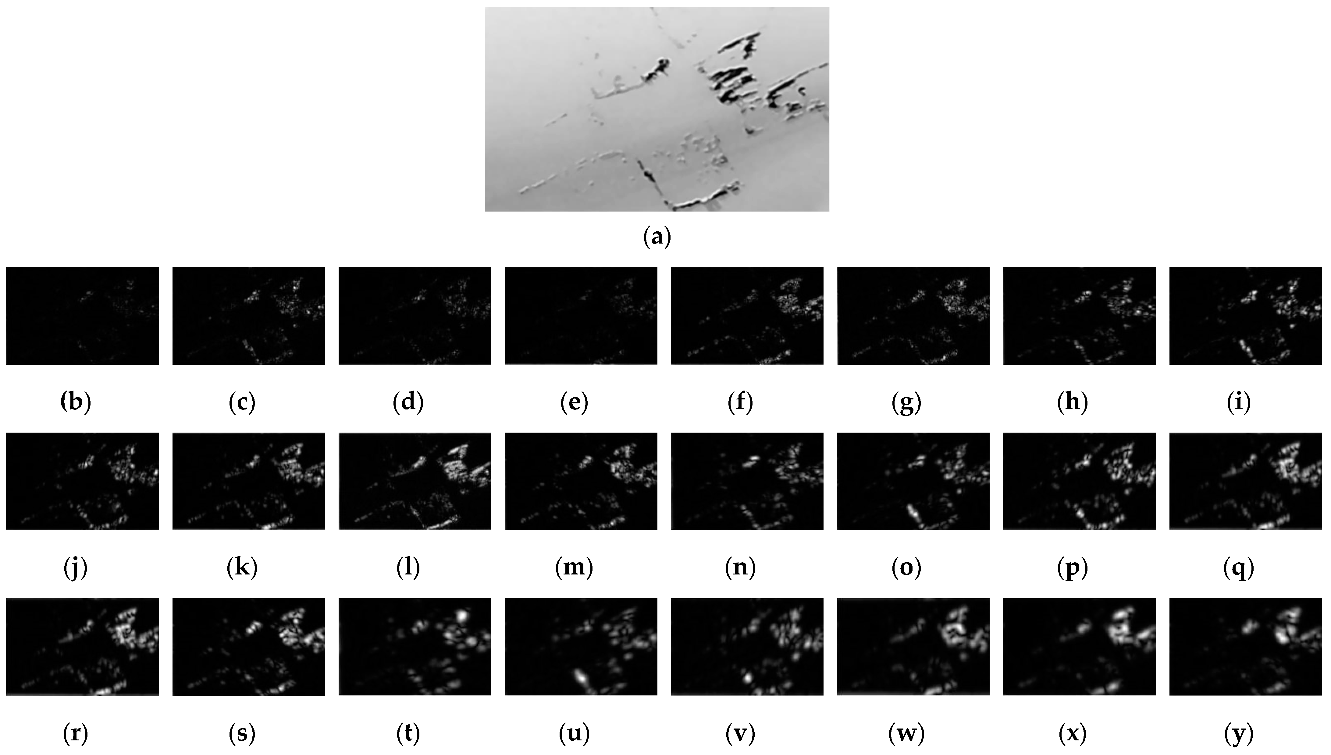
To achieve a better treatment effect, in which we put aside the workload and processing speed, we still choose four different wavelengths in the center frequency six different directions to generate the 24 different templates for processing, a scale of 4 (i.e., four different center frequencies), a direction to choose 6 different values, and a center frequency less than 2.5. The center frequencies f₀ (from left to right in Figure 9) were selected as 1/2, 1/5, 1/12.5, and 1/31.25, and the direction θ₀ (from top to bottom in Figure 9) was selected as 0, 30, 60, 90, 120, and 150. The 24 templates were used to convolve with the image respectively, and the results are shown in Figure 9.

In Figure 9b–y are the output images taken with the 24 templates.

To more intuitively observe the contrast results of the sharpness of each image after feature extraction using this method, we also calculated the average gradient value of the 24 images processed by the log-Gabor filter. The results are shown in

Table 3. The average gradient value of the 24 images after applying the log-Gabor filter.

—	f0 = 1/2	f0 = 1/5	f0 = 1/12.5	f0 = 1/31.25
θ0 = 0°	1.8397	4.8105	4.4452	5.2242
θ0 = 30°	4.4492	4.9924	4.3599	4.7948
θ0 = 60°	3.4320	4.6371	5.6060	4.8249
θ0 = 90°	3.0541	5.6833	5.5135	4.1957
θ0 = 120°	5.0495	6.5184	4.1957	4.9112
θ0 = 150°	5.5607	4.8111	4.9458	4.1872

.

It can be seen from the data in the table that when f₀ = 1/5 and θ₀ = 120, the average gradient value reached the maximum value of 6.5184. Therefore, when the log-Gabor filter f₀ = 1/5 and θ₀ = 120 was used for feature extraction, the edge information was clearer, and the noise was less.

3.2. Log-Gabor Defect Feature Extraction Based on the LPSO Algorithm

Particle swarm optimization (PSO) is an intelligent algorithm developed through swarm intelligence. It was mainly inspired by the predator–prey behavior of bird groups and was researched to simulate such behavior. It has been widely used in solving optimization problems.

The update of speed is mainly completed according to the following formula:

$$v_{im}^{k+1}=\omega v_{im}^k+c_1{r}_1(p_{im}^k-x_{im}^k)+c_2{r}_2(p_{gm}^k-x_{gm}^k)$$

(11)

The mathematical expression of the position update is as follows:

$$x_{im}^{k+1}=x_{im}^k+v_{im}^{k+1}$$

(12)

where $\omega$ represents the inertia weight; $m\in \left[1,M\right]$, $i\in \left[1,n\right]$; $v_{im}$ and $x_{im}$ represent the velocity and position of the $m$ particle, respectively; $c_1$ and $c_2$ are learning factors for the particle update speed; $r_1,r_2\in \left[0,1\right]$ is a random number; and $p_{im}$ and $p_{gm}$ represent the current locally and globally optimal solutions for the particle, respectively.

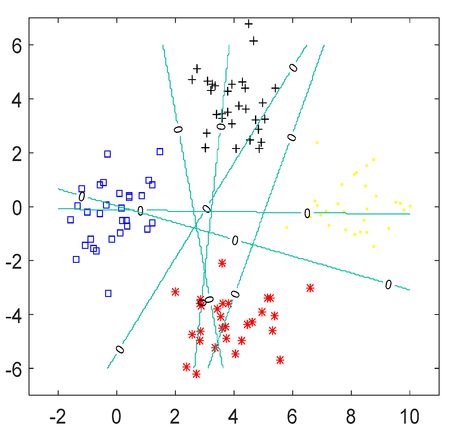
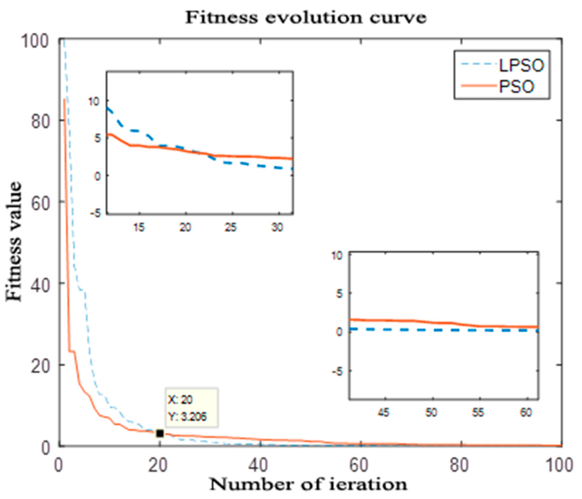
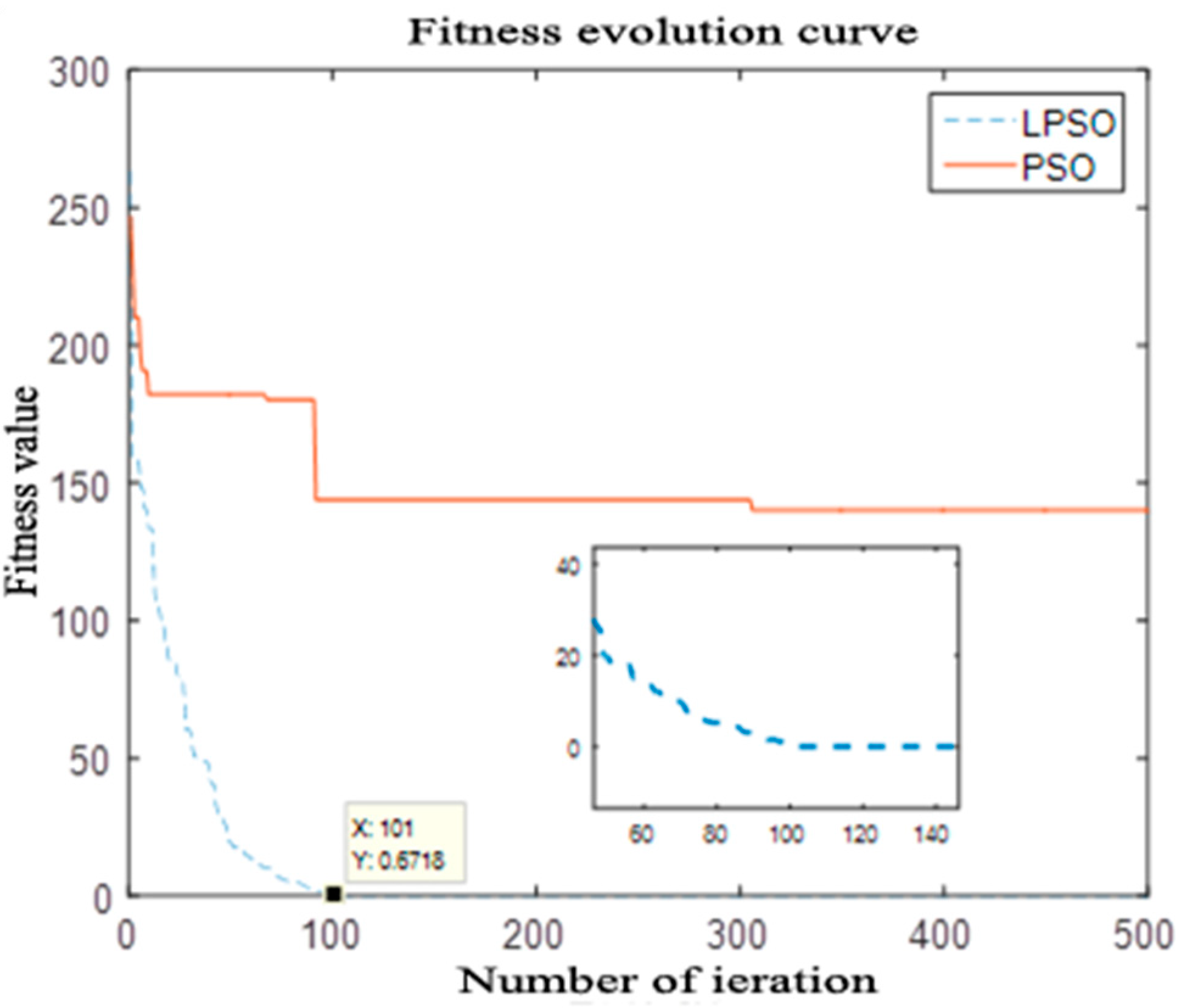
Because of the advantages of a distributed search, only a few parameters, and simple implementation, the PSO algorithm is often used to find an optimal solution. However, it also has some disadvantages, as shown in Figure 10. When it finds the optimal solution in the region, it concludes that it has found the global optimal solution. It soon stops iteration, falls into the local optimal solution, and cannot find the global optimal solution, resulting in poor solution quality.

So, we modified the PSO algorithm with the Lévy flight strategy. Lévy flight strategy is a particle flight strategy with strong randomness [28]. It initializes the spatial position of the bird flock through such random walk characteristics as frequent search at a short distance and small search at a long distance to expand the search range and enrich the population diversity, and it can jump out of the local optimal solution [29].

The variance of Lévy flight shows an exponential relationship over time. Many scholars have studied how to generate a random number that obeys the Lévy distribution. This method achieved good results and was gradually recognized by people and widely used. Thus, the method for generating random step sizes that obey Lévy’s distribution has been named after it ever since, and is known as the Mantegna algorithm. The formula can be expressed as:

$$L(\lambda )=\frac{\mu }{{\left|\nu \right|}^{-\beta }}$$

(13)

where $L\left(\lambda \right)$ represents the step length of Lévy flight; $\lambda$ is a power; $\beta$ is the learning factor of Lévy flight, usually 1.5; and $\mu$ and $v$ represent two random variables that conform to the distribution of Equation (14):

$$\left\{\begin{array}{l}\mu =N(0,{\sigma }_{\mu }^2)\\ \nu =N({\sigma }_{\nu }^2)\end{array}\right.$$

(14)

The parameter ${\sigma }_v=1$ in the above equation, and the other parameter, ${\sigma }_{\mu }$, can be obtained using Equation (15):

$${\sigma }_{\mu }=\left[\frac{\mathsf{\Gamma }(1+B)\cdot \sin (\frac{\pi \beta }{2})}{\mathsf{\Gamma }(\frac{1+B}{2})\cdot \beta \cdot 2^{\frac{\beta -1}{2}}}\right]$$

(15)

where Γ represents the standard Gamma function.

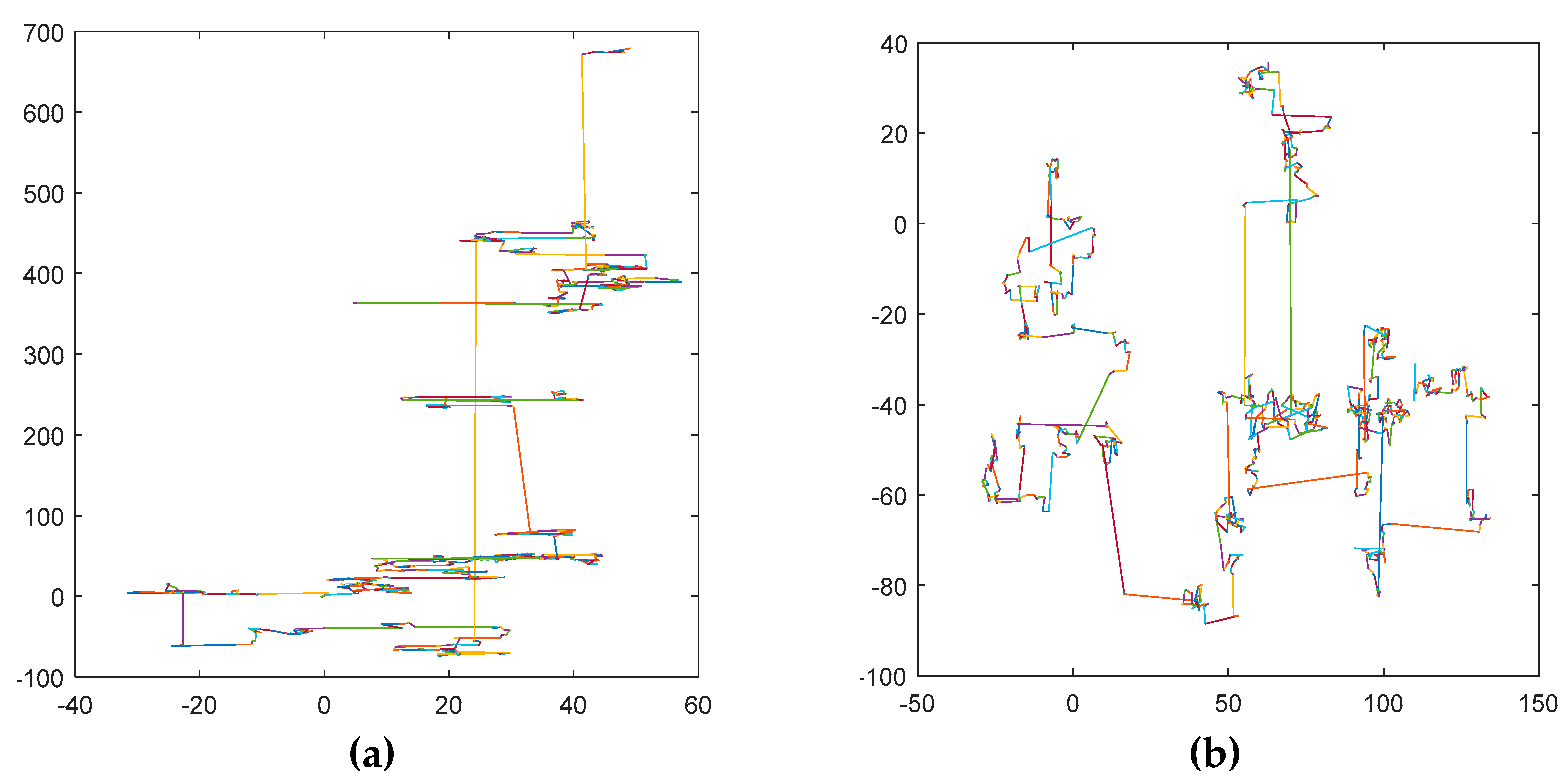
Figure 11 shows the trajectory simulation of the Lévy random flight algorithm. The left figure shows the flight trajectory of 500 iterations, and the right figure shows the flight trajectory of 1000 iterations. When observing its trajectory, it can be seen that the Lévy flight maintained its good flight characteristics after both 500 and 1000 iterations, and did not fall into the local optimal solution. However, the PSO algorithm can easily fall into the local optimal solution after a certain number of iterations.

Since Lévy flight has a good flight characteristic, in this article, the Lévy flight strategy was applied to the PSO algorithm in order to avoid using the PSO algorithm. Seeking an optimal solution from a locally optimal solution can affect the accuracy of solving the shortcomings, so it can expand the search scope in the solving process, jump out of the local optimum, and determine the global optimal solution.

The PSO algorithm improved by Lévy flight was called the LPSO algorithm. The mathematical expression of the particle velocity update is shown in Equation (16):

$$v_{im}^{k+1}=\omega v_{im}^k+c_1{r}_1(p_{im}^k-x_{im}^k)+\alpha L(\lambda )r_2(p_{gm}^k-x_{gm}^k)$$

(16)

where $\alpha$ is the step size factor.

Therefore, according to the velocity update expression, the mathematical expression of the particle position update can be obtained as shown in Equation (17):

$$x_{im}^{k+1}=x_{im}^k+v_{im}^{k+1}$$

(17)

Although the log-Gabor filter can be used to extract feature details in a very comprehensive way, the optimal parameters of different images are also different. This requires that many filters be used for each image, and the clarity of output images with different parameters is calculated and compared one by one, which leads to the low efficiency of the actual work. Therefore, an adaptive log-Gabor filter was proposed in this paper; that is, a filter could be obtained through the optimization algorithm so that the output result of this filter was the clearest, and no artificial screening was needed.

In this paper, an improved LPSO algorithm was used to improve the log-Gabor filter adaptively. According to the above, the main constituent parameters of the log-Gabor function are the center frequency $f_0$ and the direction ${\theta }_0$. So, the parameters to be adapted were $f_0$ and ${\theta }_0$. The two parameters were adjusted adaptively so that the filter could select the optimal parameters on its own for different defect images.

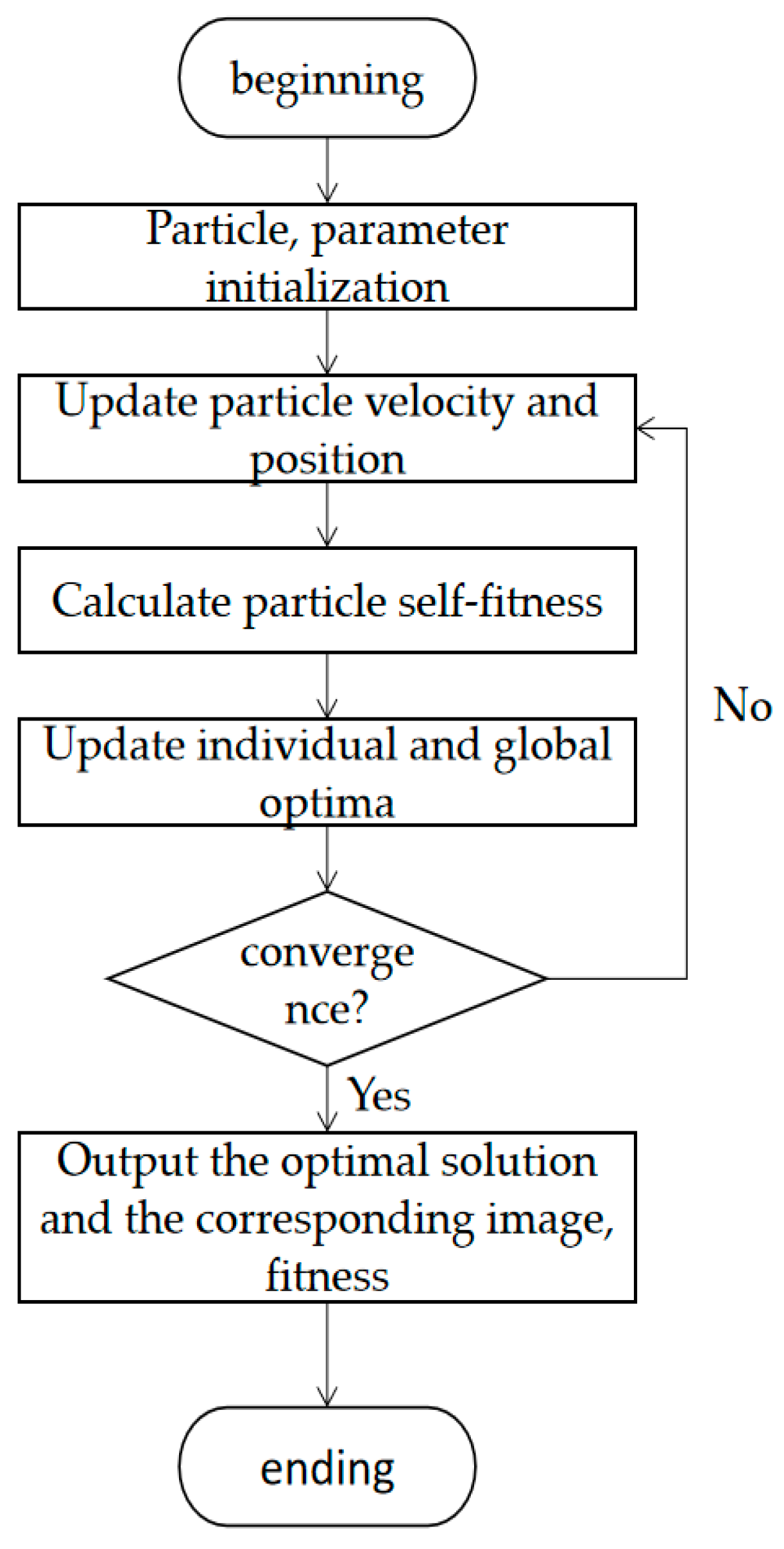
Firstly, the initial parameters of the adaptive algorithm were set. To achieve a better effect, the number of particles was selected as 50, and each particle contained a set of filter parameters, which was equivalent to generating 50 sets of filters. The initial velocity of each particle was randomly selected between −2 and 2; the initial values of the center frequency $f_0$ and radial bandwidth ${\sigma }_r$ were randomly selected between 0 and 1. The x direction was chosen randomly between 0 and ${\theta }_0$. The initial values of p_im and p_gm randomly determined were set to the initial values of the individual optimal solution and the global optimal solution.

Next, we set the fitness function, which was used to express the good or bad qualities of an individual image. In this paper, the definition of the image was determined by the average gradient value. The higher the average gradient was, the better the result of feature extraction, and the clearer the image was. Our goal was to find an image with the highest resolution and the most detailed information. At this point, the adaptive optimization filter we designed could be understood as a function aimed at solving the maximum value of the function. The average gradient value could be used as the criterion of the output result. Therefore, we could generate a fitness function employing the average gradient value function of the image. The mathematical expression for the mean gradient was briefly mentioned above, and is explained in detail here.

The mathematical expression of the average gradient value is shown in Equation (18):

$$\nabla G={\displaystyle \sum _{s_m}^{s_M}{\displaystyle \sum _{s_n}^{s_N}{(S(s_m,s_n)-\overline{S})}^2}}$$

(18)

where $\overline{S}$ represents the average gradient of the gradient image $S$; and the table $S\left(s_m,s_n\right)$ shows the gradient of the image at the point $\left(s_m,s_n\right)$. This can be expressed as follows:

$$S(s_m,s_n)=\sqrt{G_x{(s_m,s_n)}^2+G_y{(s_m,s_n)}^2}$$

(19)

where $G_x$ and $G_y$ respectively represent the gradient of the image in the $s_m$ and $s_n$ directions obtained by the Sobel gradient operator.

According to the definition of the average gradient, the higher the output average gradient is, the higher the definition will be. The above formula was used to solve the problem of the maximum, so when using an adaptive algorithm, we could take the reciprocal value, select the average gradient as the fitness function, and solve the convergence problem of the minimum; therefore, for this problem, we set the fitness function as the type shown in (20):

$$H=\frac{1}{{\displaystyle \sum _{s_m}^{s_M}{\displaystyle \sum _{s_n}^{s_N}{(S(s_m,s_n)-\overline{S})}^2}}}$$

(20)

where $H$ represents the fitness value.

Finally, we set the convergence conditions. In this problem, since the average gradient value was positive, the fitness function was always set as positive, and what we needed was a higher clarity; that is, the lower the fitness value in this paper, the better it would meet the standards of this paper. Therefore, no specific restriction was made on fitness, so only the convergence condition was set as the number of iterations. When the number of iterations reached the set value, the current global optimal solution and fitness at this time could be outputted. The basic flow chart for designing an adaptive log-Gabor filter is shown in Figure 12:

3.3. Defect-Type Detection

After feature extraction, binary images often still have some subtle miscellaneous points, and sometimes the edge information is not coherent enough, which will affect the accuracy of type judgment. To filter out the clutter and make the edge information smooth and coherent, the morphological processing method was used. Morphological processing can be divided into expansion, corrosion, open operation, and closed operation. The following four methods were introduced:

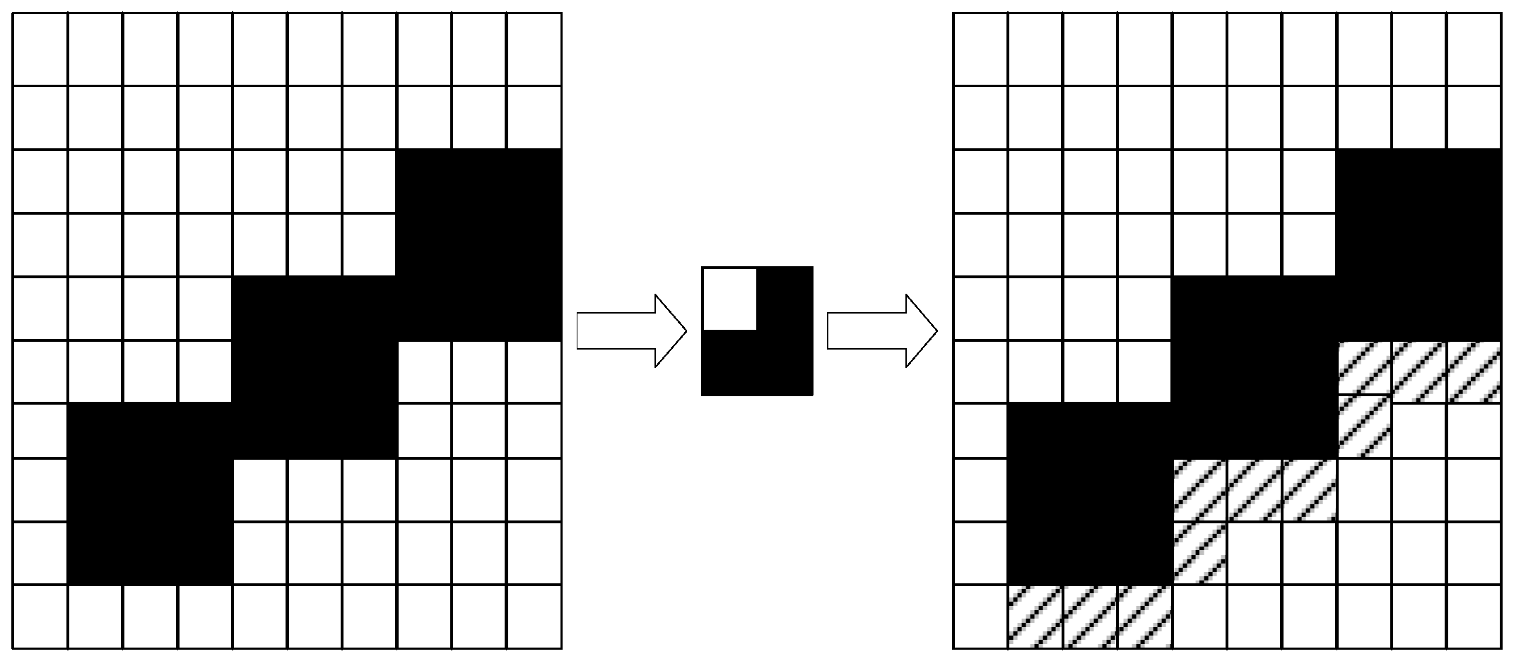
1. Expansion

The main function of expansion is to eliminate the clutter in feature areas extracted from binary images, fill in the gaps between useful information, make the lines of feature areas smooth and continuous, and highlight the area of interest more. The mathematical expression is as follows:

$$A\oplus B=\left\{x,y\left|{(B)}_{x,y}\cap A\ne \varnothing \right.\right\}$$

(21)

The principle of expansion is shown in Figure 13.

In the figure, the black and white boxes represent black and white pixels, and the dotted boxes represent pixels that have been expanded and filled.

Therefore, Formula (21) can be understood as: A was the feature image to be expanded, and we used structural element B to expand image A by placing the origin of structural element B on the position of the point in image A, obtaining the maximum value of the pixel point in the area covered by B, and assigning this maximum value to the specified pixel.

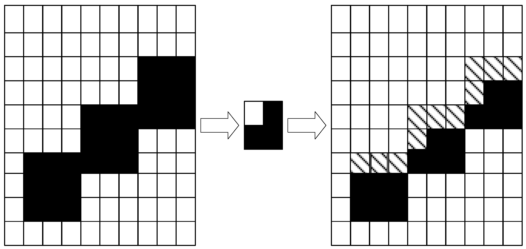
2. Corrosion

Corrosion is the main function of the binary image, including the characteristics of the region outside of the background on some useless eliminate miscellaneous points, leaving only useful features. The mathematical expression for corrosion operations is as follows:

$$A\mathsf{\Theta }B=\left\{x,y{\left|(B)\right.}_{x,y}\subseteq A\right\}$$

(22)

The corrosion principle is shown in Figure 14:

The black and white boxes in the figure represent black and white pixels, and the dashed boxes represent pixels that have been corroded away.

Formula (22) can be understood as using structure B to corrode image A. We placed the origin of structural element B at the position of the points in image A. If the element position of 1 in B was all white at the corresponding midpoint of A, then the value of the output image at the corresponding point was white; otherwise, the value was black. This is the opposite of expansion.

3. Open operation

In the combination of expansion and corrosion operations, the image is first corroded, and then expanded. The expression is as follows:

$$A\circ B=A\mathsf{\Theta }B\oplus B$$

(23)

4. Closed operation

Although understood in a similar way to an open operation, the principle is the opposite. A closed operation is an operation in which the image is first expanded and then corroded. The expression for the closed operation is shown below:

$$A•B=A\oplus B\mathsf{\Theta }B$$

(24)

Since the purpose of this paper was to extract the defective part and make a type judgment, to determine the accuracy of the defect, we needed to eliminate the useless information and highlight the defective part. Firstly, we needed to use the corrosion operation to corrode the useless elements, which was similar to the filtering process. The expansion operation was then used to connect the breakpoints and unclear points on some characteristic line segments.

As the number of connected regions was needed in the following defect type detection, the number of connected regions was identified to determine whether there was a defect, and the calculation of defect edge circumference also was used. Therefore, after the operation, the edge information of the feature was extracted to lay a foundation for the subsequent work.

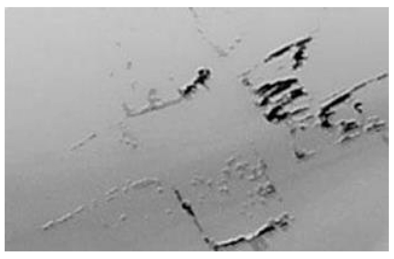
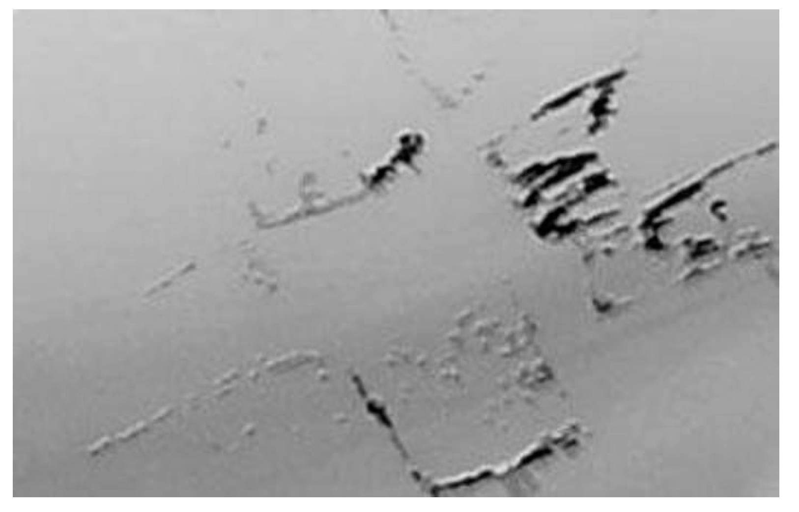
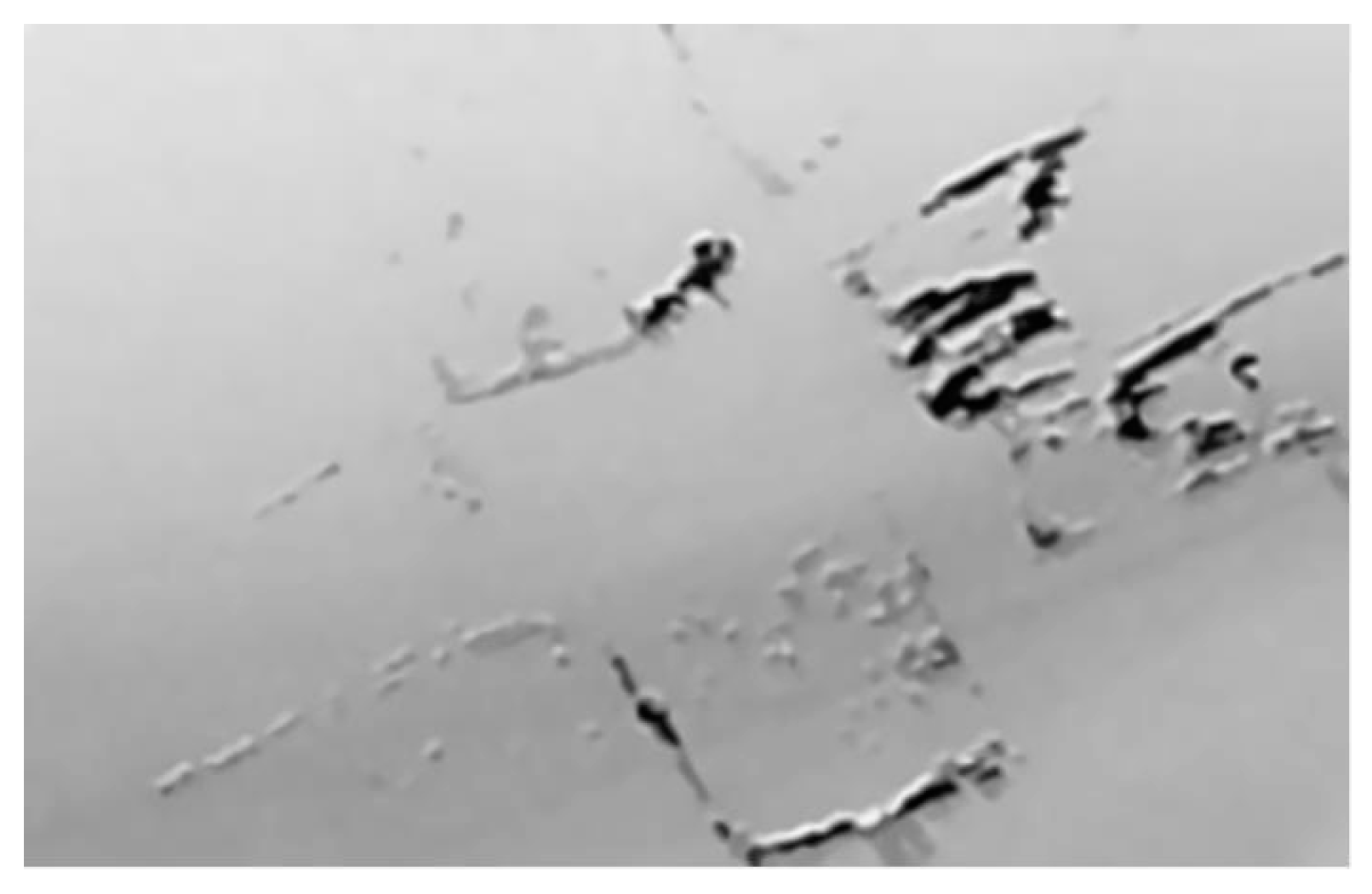
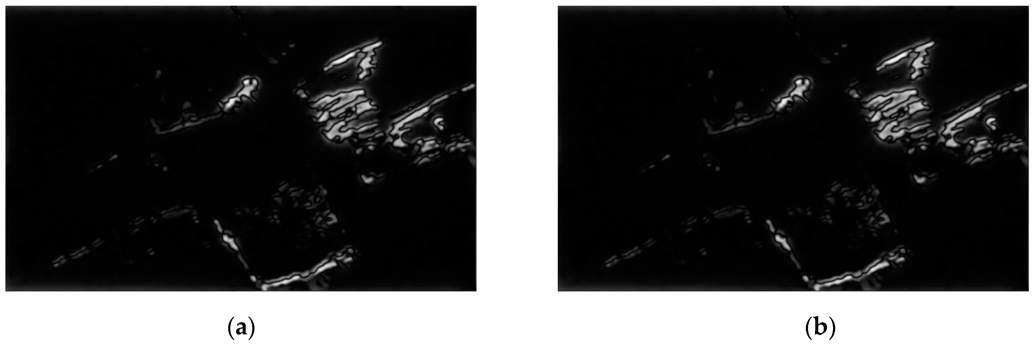
Taking the scratch image in Figure 8 as an example, the morphological processing method selected in this paper was completed for these two feature images, and the results of the open operation and extracted feature edge detection are shown in Figure 15.

As can be seen in the figure, after the operation was completed, the information in the feature area became more abundant, the defect location became more prominent, and some small useless points were filtered out. By observing the edge images obtained, it was found that this method could extract the edges of defects and form connected regions one by one. By calculating the number of connected regions, it could determine whether the image had defects. If the connected regions were not 0, it meant that the image had defects. This was used to screen whether the image had defects or not.

Defect-type detection is a process of classifying images by analyzing various attribute information of images and taking them as a classification basis. So far, the categories of classifiers are very complex. In this paper, the HOG+SVM classifier was used to classify leaf defects.

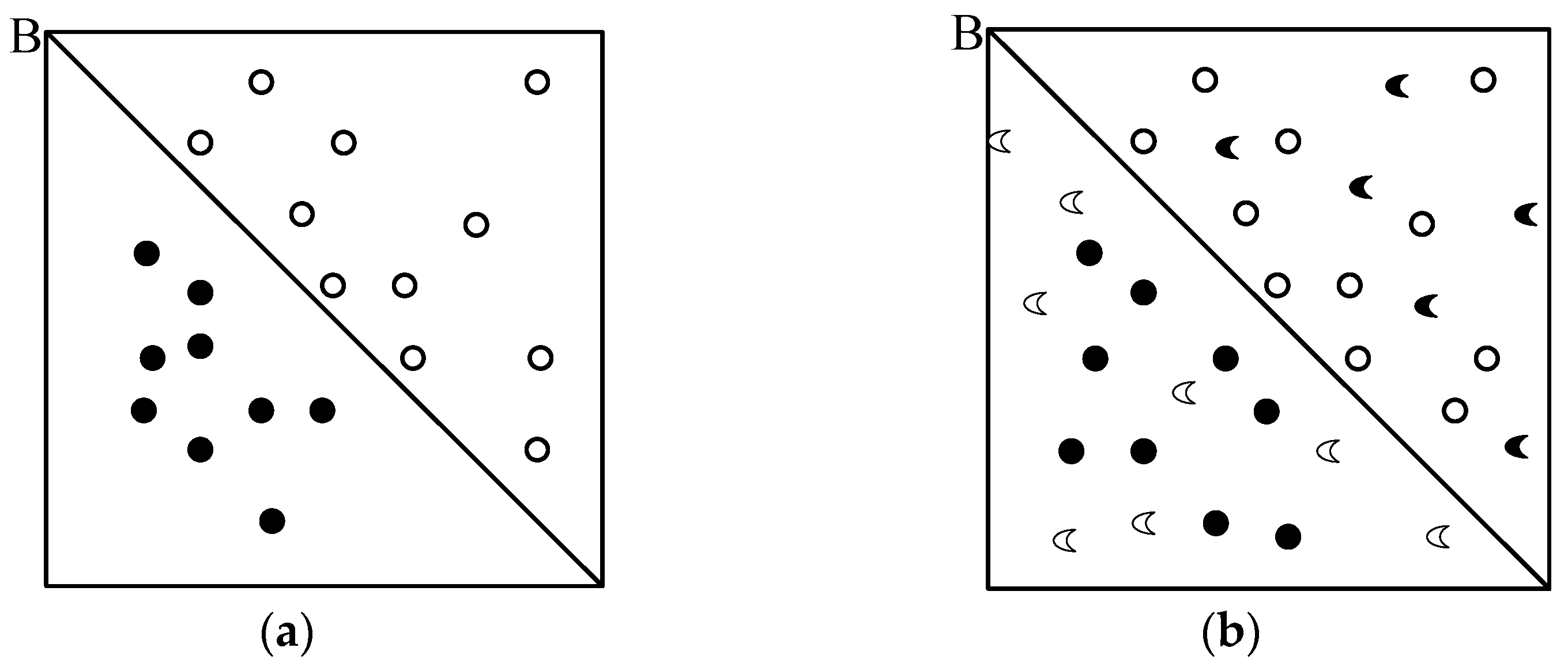
A support vector machine (SVM) classifier is a binary classifier and a supervised learning model in the field of machine learning. It is usually used to complete pattern recognition, classification, and regression analysis. It is divided into the training stage and testing stage. The main principle is to find a hyperplane between the two classes and separate the two classes by linear or nonlinear separation, as shown in Figure 16.

Figure 16a shows a classical SVM dichotomy model, while Figure 16b shows an SVM multi-classification model; B denotes the hyperplane used to divide. This hyperplane satisfies the formula:

$$\omega x-b=0$$

(25)

It is considered that the online part is 1 and the offline part is −1. The two ends of the plane are enlarged and distinguished by the positive and negative poles.

As a feature descriptor, the histogram of oriented gradient (HOG) is mainly used for object detection in visual and image processing. The HOG feature calculates and collects the histogram of the gradient direction of the local area of the image and combines these features into feature vectors. Its main working principle is to divide the image into each cell unit, collect the orientation histogram of the gradient or edge density of each cell point, and combine the collected histogram information into feature vectors, which can be used as the basis to describe the image features.

The main step of combining the two to generate a HOG+SVM classifier for binary classification was to input the positive and negative sample sets to be trained. Then, the positive and negative sample sets were read to calculate the HOG feature; the feature vector was then synthesized by the HOG feature and put into the SVM classifier for training, and the detection factor was generated. Finally, the positive and negative sample sets were put into the SVM classifier for training, and the training results were saved.

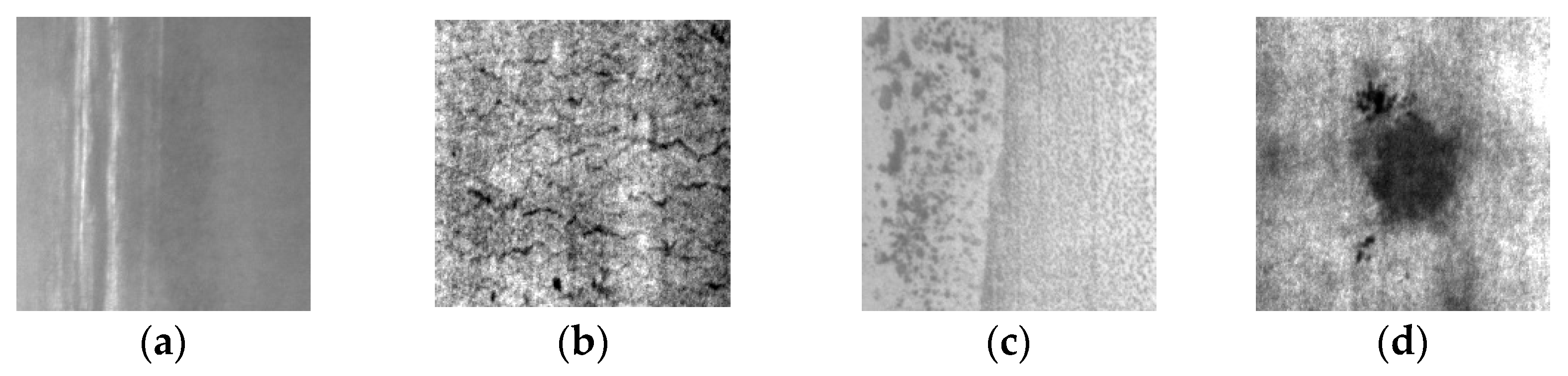
Due to the binary nature of the SVM classifier, the defect types that needed to be distinguished in this paper could be divided into four categories: spot type, sand-hole type, crack type, and scratch type. Therefore, the concept of the SVM multi-classifier was introduced, and a four-classifier system that met the requirements of this paper was designed. The basic idea of the quadclassifier was to divide the four categories into two groups of complementary classification sets. As shown in Figure 16b, the online part was considered as 1, while the offline part was −1.

According to this principle, every two different categories of the four categories are divided once to generate six training sets, namely six classical binary classifiers. When training type 1 was used, the sample set containing type 1 was positioned as a positive sample set, and the sample set not containing type 1 was defined as a negative sample set. These six binary classifiers were trained separately. During the test, when an image of type 1 was inputted, if the output results of the classifier containing type 1 were all positive, the image could be considered to belong to class 1.

The main steps of the HOG+SVM quadclassifier designed in this paper were as follows:

• Step 1: Input four sample sets;
• Step 2: Generate six different training sets and calculate the HOG feature of each training set;
• Step 3: Put the HOG feature into the SVM quadclassifier for training and generate detection factors;
• Step 4: Input the positive and negative sample sets of class I (I = 1, 2, 3, 4) into the SVM quadclassifier for training;
• Step 5: Save the training results and output the accuracy rate.

After the above steps, we tested and outputted the judgment accuracy of each type, and saved the training results. When entering the program, the training results could be directly called to input an image to be tested, and then the category to which the image belonged was outputted. The simulation results are shown in Figure 17.

4. Analysis of Experimental Results

4.1. Experiment and Analysis of Adaptive Log-Gabor Filter

Since this algorithm had two parameters to be optimized, it was equivalent to using the PSO algorithm to solve the binary function minima problem. Before the combination of the LPSO algorithm and the log-Gabor algorithm for feature extraction, to intuitively observe the comparison between the PSO and LPSO algorithms and illustrate the advantages and disadvantages of the improved LPSO algorithm, we selected two classic test functions in MATLAB, and completed the test and comparison of the algorithm before and after optimization through the MATLAB simulation. The first function was the Sphere, and the other was the Rastrigin, which are used as the representative of typical unimodal and typical multimodal functions, respectively. Both functions are known to obtain the optimal solution of the function $x_i=0$.

For the convenience of comparison, the same dimension D was selected for these two functions, both of which were 20; The number of particles was set to 50. The following simulation experiment was carried out:

1.

The mathematical expression of the Sphere function was as follows:

$$f_1(x)={\displaystyle \sum _{i=1}^n{x}_i^2}$$

(26)

Among them, $-5.12<x_i<5.12$.

The number of iterations T to be solved by the Sphere function was 100, the inertia weight $\omega$ was 0.8, and the initial velocity range was $2<v_0<2$. The fitness curve of the Sphere function is shown in Figure 18.

2.

The mathematical expression of the Rastrigin function is as follows:

$$f_2(x)={\displaystyle \sum _{i=1}^n(x_i^2-10\cos (2\pi x_i)+10)}$$

(27)

Among them, $-5.12<x_i<5.12$.

Similarly, the inertia weight of the selected Rastrigin function was 0.8. However, due to the complexity and slow solving speed of the bi-modal function, the number of iterations was increased to 500, while the initial speed range was still $2<v_0<2$. The fitness curve obtained is shown in Figure 19:

Here, we analyze the fitness curve from two aspects:

(1) In terms of stability, for these two fitness curves, it is obvious that the LPSO algorithm had good robustness, while the PSO algorithm had poor robustness, especially in multi-peak functions.

(2) From the perspective of convergence speed, the Sphere function using the LPSO algorithm was better than the PSO for the early convergence rate, but in the second half of the number of iterations after more than 20 times, the LPSO algorithm’s convergence rate was significantly higher than the PSO. When the number of iterations reached 45 times, the LPSO algorithm had determined the optimal solution, but the unimproved PSO algorithm was still in the process of seeking an optimal solution; When the Rastrigin function was solved by the LPSO algorithm, the convergence rate was significantly higher than that of the PSO algorithm. When the number of iterations reached 100, the Rastrigin function tended to the optimal solution, while the latter did not obtain the optimal solution after 500 iterations. In the second half of the function, after several MATLAB simulations, the PSO algorithm easily fell into the local optimal solution. Although the PSO algorithm was successful in solving the single-peak function, its effect was not good in seeking the extreme value of the multi-peak function. The LPSO algorithm successfully jumped out of the local optimal solution and converged to the global optimal solution $x_i=0$ in the solution of both functions. Therefore, no matter the above aspects, the improved LPSO algorithm was superior to the PSO algorithm.

The following is an example of the denoised image in Figure 8. Two improved algorithms were realized by MATLAB, and the results are shown in Figure 20.

As can be seen in the images, the image on the left is more blurred, and the boundary on the right is clearer. We then analyzed the differences between the two images through data.

Table 4. Comparison between the two adaptive feature-extraction algorithms.

—	Optimal W	Optimal Direction	Fitness
Output value based on PSO	12.0332	2.1483	0.1244
Output value based on LPSO	11.8662	2.0943	0.1172

shows the output of the optimal solution after 30 iterations.

In the table, the optimal W for the output value refers to the optimal solution of the inverse of the center frequency of the filter, while the optimal direction refers to the optimal solution of the direction angle of the filter. The inverse of the fitness here was taken to find the average gradient of the image.

An analysis of the data in Table 4 showed that although the gap between the optimal solutions obtained by the two algorithms was not very large, the optimal solution obtained by the LPSO algorithm was also slightly improved. From the perspective of the fitness value output, a small fitness value represented a high average gradient value, indicating that the image generated based on the LPSO algorithm had a higher definition. From a data point of view, by taking the reciprocal of the fitness value, the average gradient value of the image obtained based on the LPSO adaptive optimization algorithm was 8.5324. That was better than the average gradient of 6.5158 for our self-selected log-Gabor optimal image. The experimental results showed that the method was feasible.

4.2. Analysis of Experimental Results of Defect-Type Detection

In this paper, the HOG+SVM multi-classifier was implemented in MATLAB R2015b, and the data set was trained. There were a total of 1200 defect images in the existing data set, which covered the four defect types, namely spot, sand hole, crack, and scratch. There were 300 images of each type, and 250 of each type were randomly selected as training samples for a total of 1000 training samples. The remaining 200 images were reserved for the subsequent test algorithm.

Before the test, several improved algorithms proposed in this paper were used to complete the preprocessing and feature extraction of the remaining 200 images to be tested. We used the bigender function of MATLAB. The data were located in the folder for image batch reads and processes that did not improve the log-Gabor filter, based on an image fusion–Gabor filter, and based on an adaptive log-Gabor filter and several data sets, including adaptive algorithms based on the PSO and LPSO log-Gabor filter divided into two kinds for a total of four sets of data.

After training with 1000 training samples, four data sets generated after processing by different algorithms were tested and their accuracy was compared.

(1)

To improve the use of the log-Gabor feature extraction of the generated data sets, we determined the accuracy, as shown in

Table 5. The recognition accuracy of the log-Gabor feature extraction.

Type	Number of Tests to be Tested per Unit	Detected Number/Number	Accuracy/%
Spot	50	43	86%
Sand hole	50	41	82%
Crack	50	45	90%
Scratch	50	45	90%

.

(2)

With the use of feature extraction based on PSO and LPSO data sets, accuracy comparison results were obtained, as shown in

Table 6. The recognition accuracy of the log-Gabor feature extractions based on PSO and LPSO.

Type	Number of Tests per Unit	Detected Number		Accuracy/%
		PSO	LPSO	PSO	LPSO
Spot	50	45	46	90%	92%
Sand hole	50	46	48	92%	96%
Crack	50	46	46	92%	92%
Scratch	50	47	48	94%	96%

.

(3)

The recognition accuracy of other relevant methods in the literature was comparable to that of the method used in this paper, as shown in

Table 7. The accuracy of other methods in the literature compared with the method used in this paper.

Type	Reference A	Reference B	PSO	LPSO
Spot	85%	—	90%	92%
Sand hole	95%	92%	92%	96%
Crack	95%	94%	92%	92%
Scratch	95%	98%	94%	96%

. For reference A [17], the Gabor filtering method was used, and for reference B [20], the region processing method was used.

5. Conclusions

We have proposed an adaptive filter based on an improved LPSO algorithm and log-Gabor filter that could directly output multiple defect features to extract the best results from an image, and then used a HOG+SVM classifier to judge the defect type. This method could more effectively obtain accurate defect feature information, so as to improve the accuracy of defect classification. When dealing with sand-hole, spot, and crack defects, the filtering method improved by LPSO had a higher accuracy. Since the improved adaptive filter only selected the optimal result from a group of outputted parameters, the results of feature extraction were affected by the filter angle and bandwidth, but the information points were not necessarily complete when the result was optimal. Therefore, the scratch or spot information may be “smaller and thinner”, which may lead to misclassification. Therefore, obtaining more comprehensive defect feature information should be the direction of future research. In the design of the adaptive log-Gabor feature extraction algorithm, in order to obtain higher image clarity and richer feature information, the processing time was not considered, which led to an excessive processing time. Therefore, methods to simplify the process, shorten the time, and retain the feature accuracy remain to be studied.

References

1. Wang, L.; Zhang, Z. Automatic detection of wind turbine blade surface cracks based on UAV-taken images. IEEE Trans. Ind. Electron. 2017, 64, 7293–7303. [Google Scholar] [CrossRef]
2. Wang, X. Discussion on wind turbine technology development trend. Technol. Mark. 2019, 26, 161. [Google Scholar]
3. Chady, T.; Sikora, R.; Lopato, P.; Psuj, G.; Szymanik, B.; Balasubramaniam, K.; Rajagopal, P. Wind turbine blades inspection techniques. Organ 2016, 5, 16. [Google Scholar] [CrossRef] [Green Version]
4. Bo, T.; Jianyi, K.; Shiqian, W. Review of surface defect detection based on machine vision. J. Image Graph. 2017, 22, 1640–1663. [Google Scholar]
5. Ackermann, T.; Söder, L. Wind energy technology and current status: A review. Renew. Sustain. Energy Rev. 2000, 4, 315–374. [Google Scholar] [CrossRef]
6. Chu, H.-H.; Wang, Z.-Y. A vision-based system for post-welding quality measurement and defect detection. Int. J. Adv. Manuf. Technol. 2016, 86, 3007–3014. [Google Scholar] [CrossRef]
7. Yang, S.; Yang, P.; Wang, F.; Cao, H. Research on Defects and Nondestructive Testing Technology of Large-scale Wind Power Blade. Dongfang Turbine 2012, 10, 26–34. [Google Scholar]
8. Yang, R.; He, Y.; Zhang, H. Progress and trends in nondestructive testing and evaluation for wind turbine composite blade. Renew. Sustain. Energy Rev. 2016, 60, 1225–1250. [Google Scholar] [CrossRef]
9. Tian, F.; Hao, Y.; Zou, Z.; Zheng, Y.; He, W.; Yang, L.; Li, L. An ultrasonic pulse-echo method to detect internal defects in epoxy composite insulation. Energies 2019, 12, 4804. [Google Scholar] [CrossRef] [Green Version]
10. Han, K.; Hu, G.; Ren, J.; He, H.; Liu, J. Application of Image Processing in Wind Turbine Blade Flange End Face Feature Size Detection. Comput. Sci. 2019, 46, 562–565. [Google Scholar]
11. Chen, B.; Liu, H.; Meng, F. Present situation and development direction of digital image processing technology. Nat. Sci. Ed. 2009, 30, 63–70. [Google Scholar]
12. Luo, Q.; Fang, X.; Liu, L.; Yang, C.; Sun, Y. Automated Visual Defect Detection for Flat Steel Surface: A Survey. IEEE Trans. Instrum. Meas. 2020, 69, 626–644. [Google Scholar] [CrossRef] [Green Version]
13. Li, Z.; Li, H.; Sun, J. Printed circuit board defect detection based on digital image processing. Instrum. Technol. Sens. 2012, 87–89. [Google Scholar]
14. Chen, R.; Ren, D.; Yan, Z.; Gao, Y.; Fu, X. Machine vision-based defect detection system for injection empty bottles. Technol. Innov. 2018, 13–15. [Google Scholar]
15. Czimmermann, T.; Ciuti, G.; Milazzo, M.; Chiurazzi, M.; Roccella, S.; Oddo, C.M.; Dario, P. Visual-based defect detection and classification approaches for industrial applications-A SURVEY. Sensors 2020, 20, 1459. [Google Scholar] [CrossRef] [PubMed] [Green Version]
16. Tong, Z.; Yuan, D.; Gao, J.; Wang, Z. Pavement defect detection with fully convolutional network and an uncertainty framework. Comput. Aided Civ. Infrastruct. Eng. 2020, 35, 832–849. [Google Scholar] [CrossRef]
17. Qiu, Z. Defect Recognition of Wind Turbine Blade Based on UAV Image. Power Technol. 2018, 39, 277–285. [Google Scholar]
18. Kumar, P.P.; Rao, I.K. Log Gabor filter based feature detection in image verification application. Int. J. Sci. Res. 2014, 3, 703–707. [Google Scholar]
19. Jin-Feng, W.; Zhao, G.; Zhai, X.-Q.; Feng, L.-J. Study on the Improved PSO Algorithm Used in Coal Mine Safety Resource Allocation. In Proceedings of the 23rd International Conference on Industrial Engineering and Engineering Management 2016, Wuhan, China, 17–18 September 2016; pp. 149–156. [Google Scholar]
20. Márquez, F.P.G.; Tobias, A.M.; Pérez, J.M.P.; Papaelias, M. Condition monitoring of wind turbines: Techniques and methods. Renew. Energy 2012, 46, 169–178. [Google Scholar] [CrossRef]
21. Rao, Y.; Xiang, B.J.; Huang, B.; Mao, S. Wind Turbine Blade Inspection Based on Unmanned Aerial Vehicle (UAV) Visual Systems. In Proceedings of the 2019 IEEE 3rd Conference on Energy Internet and Energy System Integration (EI2), Changsha, China, 8–10 November 2019; pp. 708–713. [Google Scholar]
22. Zhao, C.; Guo, H.; Guo, T.; Liang, G. A fan blade image collection and defect detection system. Infrared Technol. 2020, 42, 1203–1210. [Google Scholar]
23. Mo, H.; Farid, G. Nonlinear and adaptive intelligent control techniques for quadrotor uav—A survey. Asian J. Control 2019, 21, 989–1008. [Google Scholar] [CrossRef]
24. Parmar, J.; Kaushal, L. Drive Fatigue Detection and Alerting System using MATLAB. Int. J. Sci. Res. Rev. UGC J. 2019, 4, 80–87. [Google Scholar]
25. Salama, A.; Smarandache, F.; ElGhawalby, H. Neutrosophic approach to grayscale images domain. Neutrosophic Sets Syst. 2018, 21, 13–19. [Google Scholar]
26. Li, P.; Liu, X. Bilinear interpolation method for quantum images based on quantum Fourier transform. Int. J. Quantum Inf. 2018, 16, 1850031. [Google Scholar] [CrossRef]
27. Kadhim, H.A.; Araheemah, W.A. A Comparative Between Corner-Detectors (Harris, Shi-Tomasi & FAST) in Images Noisy Using Non-Local Means Filter. J. Al-Qadisiyah Comput. Sci. Math. 2019, 11, 86–93. [Google Scholar]
28. Haklı, H.; Uğuz, H. A novel particle swarm optimization algorithm with Levy flight. Appl. Soft Comput. 2014, 23, 333–345. [Google Scholar] [CrossRef]
29. Yang, W.; Ma, X.; Bian, X. Adaptive improved bird flock algorithm based on Levy flight strategy. J. Hebei Univ. Technol. 2017, 46, 10–16, 22. [Google Scholar]
Figure 1. Typical images of defects: (a) scratch; (b) crack; (c) excoriation; (d) a blade cracked by lightning.
Processes 09 01452 g001
Figure 2. Four types of defects: (a) the nick type; (b) the crack type; (c) the blister type; (d) the spot type.
Processes 09 01452 g002
Figure 3. A collected blade image.
Processes 09 01452 g003
Figure 4. A region of interest for extraction.
Processes 09 01452 g004
Figure 5. An image of the region of interest.
Processes 09 01452 g005
Figure 6. The result of conversion to grayscale.
Processes 09 01452 g006
Figure 7. The image after bicubic interpolation.
Processes 09 01452 g007
Figure 8. Result after using the NL-means filter.
Processes 09 01452 g008
Figure 9. The images resulting from the log-Gabor filter: (a) is the original defect drawing; (by) are 24 feature extracted output images.
Processes 09 01452 g009
Figure 10. The PSO algorithm fell into the local optimal solution.
Processes 09 01452 g010
Figure 11. Trajectory simulation of Lévy flight: (a) 500 iterations of flight trajectory; (b) 1000 iterations of flight trajectory.
Processes 09 01452 g011
Figure 12. A flow chart for the adaptive log-Gabor function.
Processes 09 01452 g012
Figure 13. A diagram of the principle of expansion.
Processes 09 01452 g013
Figure 14. A diagram of the principle of corrosion.
Processes 09 01452 g014
Figure 15. The images resulting from the morphological processing: (a) scratch original; (b) scratch chart after opening operation chart; (c) scratch pattern edge.
Processes 09 01452 g015
Figure 16. (a) The classic SVM model; (b) the SVM multiple-classification model.
Processes 09 01452 g016
Figure 17. Visual model of the SVM quadclassifier.
Processes 09 01452 g017
Figure 18. The fitness curve of the Sphere function.
Processes 09 01452 g018
Figure 19. The fitness curve of the Rastrigin function.
Processes 09 01452 g019
Figure 20. Comparison of two adaptive feature extraction algorithms: (a) output image based on PSO; (b) output image based on LPSO.
Processes 09 01452 g020