Optimization of a Multi-Energy Complementary Distributed Energy System Based on Comparisons of Two Genetic Optimization Algorithms

Abstract

The development and utilization of low-carbon energy systems has become a hot topic of energy research in the international community. The construction of a multi-energy complementary distributed energy system (MCDES) is researched in this paper. Based on the multi-objective optimization theory, the planning optimization of an MCDES is studied, and a three-dimensional objective-optimization model is constructed by considering the constraints of the objective function and decision variables. Aiming at the optimization problem of building terminals for the MCDES studied in the paper, two genetic optimization algorithms—Non-Dominated Sorting Genetic Algorithm II (NSGA-II) and Non-Dominated Sorting Genetic Algorithm III (NSGA-III)—are used for calculation based on an example analysis. The constraint conditions of practical problems were added to the existing algorithms. Combined with the comparison of the solution quality and the optimal compromise solution of the two algorithms, a multi-decision method is proposed to obtain the optimal solution based on the Pareto optimal frontier of the two algorithms. Finally, the optimal decision scheme of the example is determined and the effectiveness and reliability of the optimization model are verified. Under the application of the MCDES optimization model studied in this paper, the iteration speed and hypervolume index of NSGA-III are found to be better than those of NSGA-II. The values of the life cycle cost and life cycle carbon emission objectives after the optimization of NSGA-III are indicated as 2% and 14% lower, respectively, than those of NSGA-II. The primary energy efficiency of NSGA-III is shown to be 20% higher than that of NSGA-II. According to the optimal decision, the energy operation strategies of the example MCDES with each typical day in the four seasons indicate that good integrated energy application and low-carbon operation performance are shown during the four-seasons operation process. The consumption of renewable energy is significant, which effectively reduces the application of high-grade energy. Thus, the theoretical guidance and engineering application reference are provided for MCDES design planning and operation optimization.

1. Introduction

An MCDES, which is formed by the organic coordination and optimization of energy generation, transmission, distribution, conversion, storage, and consumption, is an integrated system with energy production, supply, and marketing. It is composed of basic units such as supply side, conversion side, and demand side. Many kinds of energy such as power, gas, and renewable energy in the supply side, are transformed into the energy directly consumed by users in the demand side through the technical transformation of the conversion side. A green, efficient, and stable MCDES is considered to be the main bearing form of future social energy.

In terms of improving the comprehensive energy efficiency, the effective utilization of renewable energy and energy storage equipment can make an MCDES give full play to the advantages of different energy coupling and complementary approaches. Emara et al. [1], based on photovoltaic modules and battery energy storage systems, proposed the enhanced operation control strategy of a DC microgrid system under two different operation modes: standalone, and grid-connected. Six different scenarios of the system were simulated. The results show that the photovoltaic power generation is changed by changing the irradiance level. The new control strategy enables the photovoltaic power generation system to achieve maximum power generation in the microgrid through different technologies. The battery reduces the voltage spikes and has strong load adaptability by introducing stable operation and adjustable DC voltage, and further achieves the flexibility and reliability of electricity by balancing power demand and power generation. Ali et al. [2] pointed out that the efficiency of a photovoltaic system is the key index by which to evaluate the performance of photovoltaic grid-connected power generation systems, where the MPPT performance is the key to the efficiency of the photovoltaic system. In order to improve the accuracy and convergence speed of conventional MPPT under a fixed-step-size INC, an MPPT method based on a fuzzy logic algorithm was proposed. Ali Eman et al. [3] proposed a two-stage renewable energy penetration (RES) optimization planning method for the when a high RES caused by uncertain factors such as climate deteriorates the performance and safety of the distribution system significantly. It is pointed out that, when using the multi-objective cat swarm algorithm as a solution, the voltage variation depends not only on the penetration level of renewable energy, but also on the location of the distributed generation unit. By considering the different strategies of RES in radial distribution systems and the influence of uncertainty on the distribution network voltage, the RES in an unbalanced distribution network is improved.

Because energy production and transmission equipment has a long service life in the energy industry, the carbon emission intensity will be determined by the planning scheme for a long time in the future. Once a certain initial state is determined, it will cause a long-term impact such as a carbon lock-in effect [4]. Therefore, under the perspective of low-carbon economy, and from the perspective of energy production, it is necessary to control the source so as to reduce the carbon emissions of the system in order to promote the output of renewable energy, such as hydro power, wind power, or photovoltaic power. Study of the optimization of MCDES systems is very important for social significance and engineering applications.

Currently, the studies on the optimization of MCDES system planning, structure, or configuration are generally divided into three aspects: energy grid optimization planning; renewable energy ratio, type selection, and capacity planning; and energy storage type and capacity planning [5,6,7,8]. The optimization objectives are focused on economy, reliability, and environmental protection, etc. [9,10,11,12]. Jing et al. [13], based on environmental protection and economy, optimized the capacity design of a distributed integrated energy system with photovoltaic power generation by considering the carbon emissions and investment recovery period. Mehleri et al. [14] designed an MCDES based on home cooling and heating load by using a mixed-integer linear programming method, and optimized it to determine the main equipment types and installed capacity of the system. Huang et al. [15] simplified the multi-energy system planning problem as a mixed-integer linear programming problem by constructing a hierarchical linear energy hub model and adopting a DC power flow model and piecewise linear gas network model. Bahramirads [16] constructed the optimal configuration model of the storage system based on the stability of the whole micro energy network. Jayasekara et al. [17] used a two-stage particle swarm optimization algorithm to study the optimal capacity configuration of equipment by taking the minimum annual total cost as the optimization objective. Salimi et al. [18] solved the system capacity allocation problem by establishing a multi-energy system unit with cooling, heating, and power. Lin et al. [19], considering the power interaction between multi-microgrid systems, took the total annual cost and the lowest operating cost of the system as the optimization objectives to solve the selection and sizing of multi-microgrid equipment. Pelet et al. [20] used the multi-objective optimization method to carry out system simulation by taking into account various factors—including resources, demand, energy, emissions, and costs—comprehensively, while the optimal allocation was simulated. Chang [21] proposed that the two-stage planning model can be used in multi-energy flow system planning; in the first stage, the optimization of the system structure can be completed by the target genetic algorithm; in the second stage, the solution of the optimal operation of the system can be realized by the mixed-integer programming method, and the construction of the nonlinear model can also be realized, including the P2G device and the CHP unit; after linearization, the optimization of the system is completed.

MCDESs have characteristics such as complex structure, involving multiple energy networks, large timescale gap, and strong uncertainty. Hence, the associated planning and configuration problems are much more complex than those of traditional energy systems. Therefore, the system planning optimization is a typical multi-objective optimization problem. Among many methods for solving multi-objective optimization problems, the multi-objective optimization strategy based on genetic algorithms has been widely used in various fields. Multi-objective evolutionary algorithms (MOEAs) have good effectiveness; they are global heuristic probability optimization search algorithms developed on the basis of genetic algorithms; their non-dominated sorting genetic algorithm (NSGA) series is widely used in multidimensional optimization applications. In 1995, Deb et al. proposed the NSGA for high-dimensional multi-objective problems that are difficult to solve via genetic algorithm; then, the improved NSGA-II to improve the speed of solution was proposed in 2002; the NSGA-III, with a reference point selection mechanism to improve the solution effect of multi-objective problems, so as to make up for the deficiency of convergence of the NSGA-II for crowding operator, was proposed in 2014 [22,23,24].

NSGA-II, as a relatively mature method that became a benchmark algorithm for optimizing the performance comparison of other multi-objective optimization algorithms, has been widely used. It has high solving efficiency, and can obtain multiple high-quality solutions in one calculation. As a new method for solving multi-objective optimization problems, NSGA-III has achieved good results in solving high-dimensional multi-objective optimization problems with a large number of objectives [24,25,26]; it has certain advantages in improving operation efficiency, increasing the diversity of solution space, and reducing computational complexity, which can effectively compensate for the shortcomings of other optimization algorithms. However, there are few studies on the application of NSGA-III in solving the multi-objective optimization problem of multi-energy systems at present. NSGA-III is proposed based on NSGA-II, and is superior to NSGA-II in terms of convergence speed and diversity, but different algorithms for constrained problems in practical applications will show different optimization performance due to the algorithm proposed on a simple test function [27]. When dealing with practical problems with complex constraints, it is very meaningful to consider the comparison of different algorithms for quantitative analysis, and find different measures for the frontier of non-dominated solutions [28,29,30].

Overall, a multi-objective programming optimization approach to the construction terminal of an MCDES is studied in this paper. Through example optimization, NSGA-II and NSGA-III are used to optimize the calculation. The novelty of this work is that, in view of the actual problems studied, the problem constraints are expanded in the existing algorithms. Combined with the comparison of the quality of the solution and the optimal compromise solution of the two algorithms, a multiple decision-making method based on the Pareto optimal frontier of the two algorithms is proposed for obtaining the optimal solution. Thus, the final decision scheme of the system design optimization is comprehensively determined.

2. Optimization Modeling and Methods

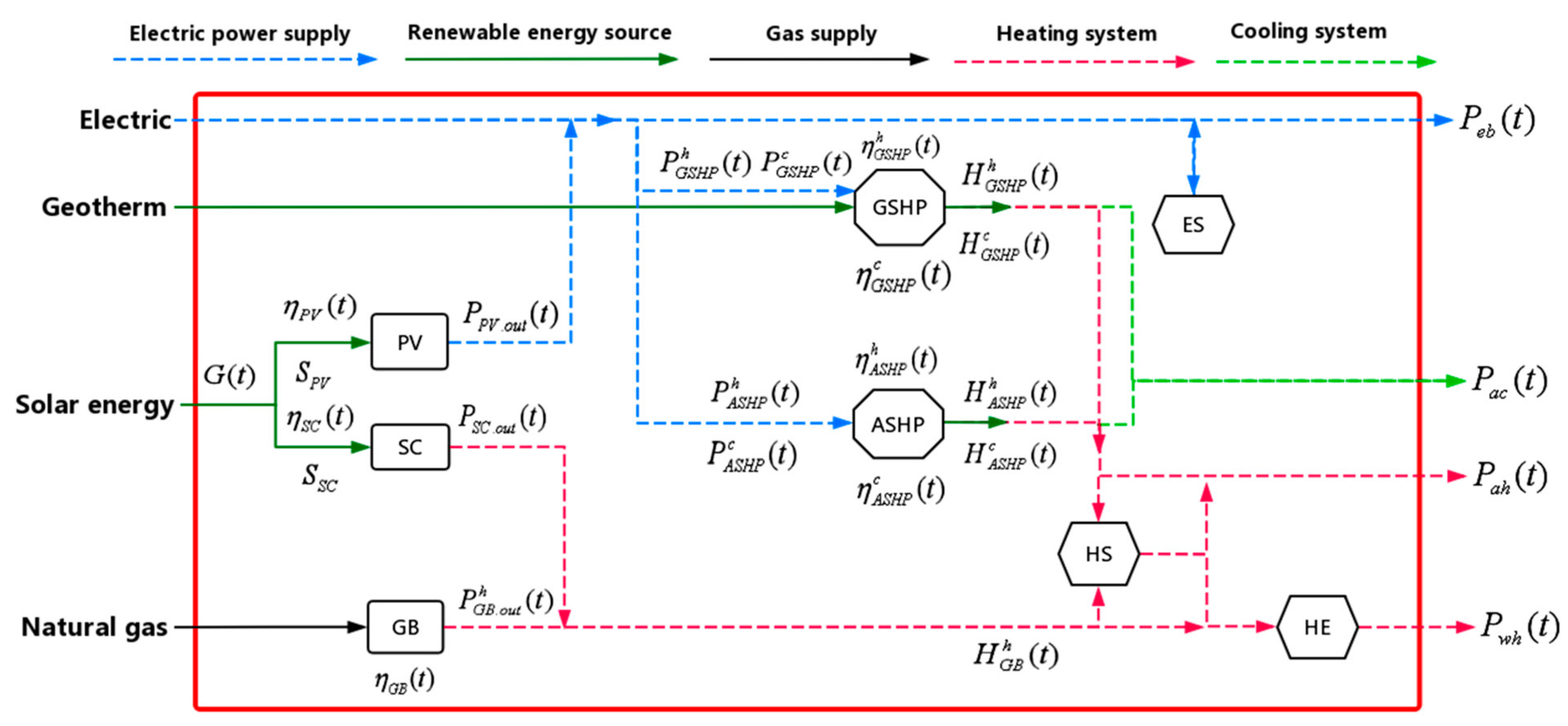
2.1. Mathematical Modeling

The basic energy supply equipment of the MCDES studied in this paper includes: photovoltaic (PV) power supply equipment; solar energy collector (SC), gas boiler (GB), ground-source heat pump (GSHP), and air-source heat pump (ASHP) as heating/cooling equipment; energy hub (EH) with electric energy storage (ES) and heat storage (HS) as energy storage equipment; and heat exchange (HE) as heat exchange equipment.

The energy supply form is shown in Figure 1.

(1) Photovoltaic Power Generation (PV)

The output power of PV systems is generally related to the solar radiation intensity and outdoor environment temperature. The influence of solar radiation intensity is only considered in the modeling. Due to the small variation range of temperature in a day, the influence of air temperature is ignored. Therefore, the predicted output power of PV depends on the area of the photovoltaic panels, light radiation intensity, and energy conversion efficiency of the photovoltaic panels. The expression under variable working conditions can be written as follows [31]:

$$P_{PV.out}(t)=G(t)S_{PV}{\eta }_{PV}(t)$$

(1)

where $P_{PV.out}(t)$ is the forecast output of PV at time t (kW); $G(t)$ is the solar radiation intensity at time t (W/m²); and $S_{PV}$ is the installation area for photovoltaic panels (m²).

${\eta }_{PV}(t)$ is the power generation efficiency of photovoltaic panels at time t, and its variable condition expression can be written as:

$${\eta }_{PV}(t)={\alpha }_1[{(\frac{G(t)}{G_0})}^{{\alpha }_2}+{\alpha }_3(\frac{G(t)}{G_0})][1+{\alpha }_4(\frac{T}{T_0})+{\alpha }_5(\frac{A}{A_0})]$$

(2)

where ${\alpha }_1$,${\alpha }_2$,${\alpha }_3$,${\alpha }_4$, and ${\alpha }_5$ are all constants, equal to 0.28204, 0.39668, −0.44730, −0.092864, and 0.016010 respectively; $G_0$ is the solar radiation intensity under standard test conditions, equal to 1000 W/m²; $T$ is the outdoor environment temperature (°C); $T_0$ is the outdoor environment temperature under standard test conditions, equal to 25 °C; $A$ is the air mass (kg); and $A_0$ is the air mass under standard test conditions, equal to 1.5 kg.

(2) Solar Energy Collector (SC)

The flat-panel solar collector absorbs solar energy through the heat absorption device and converts it into heat energy for utilization. This is the most basic type of SC, with the advantages of simple structure, low cost, and reliable operation. It is also the most widely used solar energy absorption and utilization device, with more than 90% of market share. The efficiency is related to solar radiation and the parameters of the collector itself [32,33]. Considering the variable working conditions, the predictive output formula can be expressed as:

$$P_{SC.out}(t)=G(t)S_{SC}{\eta }_{SC}(t)$$

(3)

where $P_{SC.out}(t)$ is the SC output power at time t (kW); $G(t)$ is the solar radiation intensity at time t (W/m²); and $S_{SC}$ is the installation area of photovoltaic panels (m²).

${\eta }_{SC}(t)$ is the energy conversion efficiency of the SC, and its variable condition expression can be written as:

$${\eta }_{SC}(t)=\phi \omega k-\frac{\varphi U(T_{in}-T)}{G(t)}$$

(4)

where $\phi$ is the heat transfer factor; $\omega$ is the transmittance; $k$ is the absorption rate; $U$ is the heat loss efficiency of the endothermic plate (W/m²·°C); $T_{in}$ is the collector inlet temperature (°C); and $T$ is the outdoor environment temperature (°C).

(3) Gas Boiler (GB)

A GB with relatively stable working characteristics is a kind of unit equipment with coupling conversion between gas and heat flow to meet the demand of heat load by consuming natural gas. The heat generated is related to the efficiency of the boiler. Under the influence of the change of the unit conversion efficiency over time, the mathematical model expression can be written as [34]:

$$P_{GB.out}^h(t)=P_{GB.in}^g(t){\eta }_{GB}$$

(5)

$$H_{GB}^h(t)=P_{GB.out}^h(t)\Delta t$$

(6)

where $P_{GB.in}^g(t)$, $P_{GB.out}^h(t)$, and $H_{GB}^h(t)$ are consumption of natural gas power, output heat power, and output heat value of the GB, respectively, at time t (kW); ${\eta }_{GB}$ is the thermal efficiency of the GB; while $\Delta t$ is the scheduling time.

(4) Ground-Source Heat Pump (GSHP)

GSHPs, which can provide winter heating and summer cooling, generally use a shallow geothermal heat source. Through flowing in a closed underground pipe formed as water or antifreeze and other intermediate heat transfer media with water, they absorbs low-temperature heat energy from the environment or release heat energy to the environment to output several times more heat/cold energy than their own power consumption. Therefore, heat exchange with the soil will be achieved to reduce the fossil energy consumption effectively. However, the working time mode is usually limited in terms of reducing the damage caused by the system to the environmental energy balance. The output power of the GSHP depends on the performance coefficient and load condition; its variable condition characteristics can be described as follows [35]:

① Heat supply under heating condition:

$$H_{GSHP}^h(t)=P_{GSHP}^h(t){\eta }_{GSHP}^h(t)X_{GSHP}(t)$$

(7)

where $H_{GSHP}^h(t)$ and $P_{GSHP}^h(t)$ are the heat supply and the total input power of the heating condition of the GSHP, respectively, at time t (kW); ${\eta }_{GSHP}^h(t)$ is the heating coefficient of the GSHP at time t; and $X_{GSHP}^h(t)$ is the 0–1 variable of the running state at time t, taking 1 as the running state and 0 as the shutdown state.

② Cooling capacity under refrigeration condition:

$$H_{GSHP}^c(t)=P_{GSHP}^c(t){\eta }_{GSHP}^c(t)X_{GSHP}(t)$$

(8)

where $H_{GSHP}^c(t)$ and $P_{GSHP}^c(t)$ are the cooling capacity and the total input power of the refrigeration condition of the GSHP, respectively, at time t (kW); ${\eta }_{GSHP}^c(t)$ is the refrigeration coefficient of the GSHP at time t; and $X_{{}_{GSHP}}^{}(t)$ is the 0–1 variable of the running state at time t, taking 1 as the running state and 0 as the shutdown state.

(5) Air-Source Heat Pump (ASHP)

The ASHP is basically similar to the GSHP, and the difference is that the energy sources are different. An ASHP uses air as the energy source for heating or cooling. Its variable condition characteristics can be described as:

① Heat supply under heating condition:

$$H_{ASHP}^h(t)=P_{ASHP}^h(t){\eta }_{ASHP}^h(t)X_{ASHP}(t)$$

(9)

where $H_{ASHP}^h(t)$ and $P_{ASHP}^h(t)$ are the heat supply and the total input power of the heating condition of the ASHP, respectively, at time t (kW); ${\eta }_{ASHP}^h(t)$ is the heating coefficient of the ASHP at time t; and $X_{ASHP}^{}(t)$ is the 0–1 variable of the running state at time t, taking 1 as the running state and 0 as the shutdown state.

② Cooling capacity under refrigeration condition:

$$H_{ASHP}^c(t)=P_{ASHP}^c(t){\eta }_{ASHP}^c(t)X_{ASHP}(t)$$

(10)

where $H_{ASHP}^c(t)$ and $P_{ASHP}^c(t)$ are the cooling capacity and the total input power of the refrigeration condition of the GSHP, respectively, at time t (kW); ${\eta }_{ASHP}^c(t)$ is the refrigeration coefficient of the GSHP at time t; and $X_{{}_{ASHP}}^{}(t)$ is the 0–1 variable of the running state at time t, taking 1 as the running state and 0 as the shutdown state.

(6) Electric Energy Storage (ES)

The indicators of ES equipment include equipment capacity, state of charge, and ratio of charge/discharge. The charge state of the battery is a parameter that reflects the proportion of the battery’s remaining power in the total capacity. Generally, for the battery’s safe operation, the state of charge (SOC) and state of health (SOH) estimations are essential [36]. The battery model is constructed by the relationship with the charging and discharging power and capacity of the battery. Then, the mathematical expression can be written as [36,37]:

$$SO{C}_{ES}^{}(t)W_{ES}=(1-{\delta }_{ES})SO{C}_{ES}(t-1)W_{ES}+[P_{ES}^{in}(t)*{\eta }_{ES}^{in}-\frac{P_{ES}^{out}(t)}{{\eta }_{ES}^{out}}]\Delta t$$

(11)

where $SO{C}_{ES}(t)$ and $SO{C}_{ES}(t-1)$ are the equipment charge rate at times t and t−1, respectively; $W_{ES}$ is the equipment’s rated capacity (kW); $P_{ES}^{in}(t)$ and $P_{ES}^{out}(t)$ are the charging and discharging power of the ES equipment, respectively, at time t (kW); ${\eta }_{ES}^{in}$ and ${\eta }_{ES}^{out}$ are the charging and discharging efficiency, respectively, at time t; ${\delta }_{ES}$ is the filling loss rate; and $\Delta t$ is the optimized time of the scheduling simulation step, equal to 24 h.

(7) Heat Storage (HS)

Heat storage technology is generally divided into sensible heat storage and phase-change heat storage. Similar to the energy storage battery, the heat storage state of the HS system, charging and discharging heat power, and heat storage capacity model can be expressed as [37]:

$$SO{C}_{HS}^{}(t)W_{HS}=(1-{\delta }_{HS})SO{C}_{HS}(t-1)W_{HS}+[P_{HS}^{in}(t)*{\eta }_{HS}^{in}-\frac{P_{HS}^{out}(t)}{{\eta }_{HS}^{out}}]\Delta t$$

(12)

where $SO{C}_{HS}(t)$ and $SO{C}_{HS}(t-1)$ are the equipment charge rate at times t and t−1, respectively; $W_{ES}$ is the ES equipment’s rated capacity (kW); $P_{HS}^{in}(t)$ and $P_{HS}^{out}(t)$ are the charging and discharging power of the HS equipment, respectively, at time t (kW); ${\eta }_{HS}^{in}$ and ${\eta }_{HS}^{out}$ are the charging and discharging efficiency of the HS equipment, respectively, at time t; and ${\delta }_{HS}$ is the heat loss rate.

2.2. Optimization Objectives and Constraints

The life cycle cost, life cycle carbon emissions, and system primary energy utilization are taken as the optimization objectives to optimize the MCDES planning in the paper. The optimization model is expressed as follows:

$$\{\begin{array}{l}\min F_i(x)={(f_1(x),f_2(x),-f_3(x))}^T\\ s.t\hspace{1em}{g}_i(x)\le 0\hspace{1em}i=1,2,3\\ s.t\hspace{1em}{h}_j(x)=0\hspace{1em}j=1,2,3\end{array}$$

(13)

2.2.1. Optimization Objectives

(1) Economical Objective

Because the MCDES studied in this paper is a terminal multi-energy system, only the cost factor is considered for the economic evaluation, without the benefit factor being considered. The life cycle cost is used for the index, and is converted to the equivalent annual cost. The minimum equivalent annual cost is taken as the economic optimization goal; it includes the initial investment cost in the investment period, the operation and maintenance costs in the operation stage, the multiple replacement cost in the life cycle caused by the short life cycle of energy storage equipment, and the residual cost of some equipment eliminated at the end of the system.

The expression is:

$$F_1=C_{eav}=1.3C_{eq}+{\displaystyle \sum _{t=1}^{N_t}}[C_f(t)+C_m(t)]+C_{EH.rep}-C_{RV}$$

(14)

where $C_{eav}$ is the total cost of the system life cycle (CNY); $C_{eq}$ is the investment cost for the system equipment (CNY); $C_f(t)$ represents the system operating costs at time t (CNY); $C_m(t)$ is the system maintenance cost at time t (CNY); $C_{EH.rep}$ represents the EH replacement costs (CNY); $C_{RV}$ is the total residual value for device i at the end of the planning cycle (CNY); and $N_t$ is the system planning period, equal to 20 years.

In order to simplify the calculation, the input cost of the MCDES auxiliary system is calculated as 30% of the total initial input cost of the system [38].

(2) Environmental Objective

The primary energy consumption of the MCDES comes from natural gas and electricity. The greenhouse gas emitted is CO₂. Considering the promotion of ecological environmental protection along with energy conservation and emission reduction, CO₂ emissions released by natural gas and electricity are used as the evaluation index for environmental impact. The minimum total carbon emissions of the system are taken as the environmental protection optimization goal. The specific expression formula can be written as follows:

$$F_2={\displaystyle \sum _{t=1}^{N_t}}{E}_{C{O}_2}$$

(15)

where $E_{C{O}_2}$ represents the total system carbon emissions for its life cycle (kg).

(3) Energy Efficiency Objective

The primary energy utilization is adopted to evaluate energy consumption in the text, where the primary energy includes natural gas, grid power, and renewable resources calculated as zero. Considering the consistency of the optimization direction in the optimization function, it can be expressed as:

$$F_3=-PER(t)$$

(16)

where $PER(t)$ is the system’s primary energy utilization at time t.

2.2.2. Constraint Conditions

Certain constraints should be met while the decision variables are optimized in processing. Constraints including equipment capacity constraint, equipment output constraint, energy balance constraint, and energy storage constraint are considered in the text.

(1) Constraint of Equipment Capacity

The installation capacity of each piece of equipment in the system is affected by available resources, installation site, and technology. The equipment capacity constraint is shown as follows:

$$W_{i.\min }\le W_i\le W_{i.\max }$$

(17)

where $W_i$ is the installation capacity of device i (kW); while $W_{i.\max }$ and $W_{i.\min }$ are the upper and lower limits of the installation capacity of device I, respectively (kW).

(2) Constraint of Equipment Power

For reducing the difficulty of solving the problem, the constant efficiency assumption is adopted. When modeling, it is assumed that the operation efficiency of the equipment in a given interval is constant, and when the equipment’s efficiency is lower than the lower limit of the given output interval, it is disabled [39].

$${\beta }_{i.\min }{W}_i\le P_{i.out}(t)\le {\beta }_{i.\max }{W}_i$$

(18)

where ${\beta }_{i.\min }$ and ${\beta }_{i.\max }$ are the minimum and maximum load rates allowed for device i, equal to 0.2 and 1.0, respectively; and $P_{i.out}(t)$ is the output power of device i at time t (kW).

(3) Constraint of Cooling, Heating, and Power Balance

① Power balance:

$$P_{PV.out}(t)+P_e(t)+P_{ES}^{out}(t)=P_{GSHP}^{}(t)X_{GSHP}+P_{ASHP}^{}(t)X_{ASHP}+P_{ES}^{in}(t)+P_{eb}(t)$$

(19)

② Heating balance:

$$H_{GSHP}^h(t)X_{GSHP}+H_{ASHP}^h(t)X_{ASHP}+H_{GB}^h(t)+P_{SC.out}(t)+P_{HS}^{out}(t)=P_{ah}(t)+P_{hw}(t)+P_{HS}^{in}(t)$$

(20)

③ Cooling balance:

$$H_{ASHP}^c(t)X_{ASHP}+H_{GSHP}^c(t)X_{GSHP}=P_{ac}^{}(t)$$

(21)

(4) Constraint of EH

In addition to the formula charge constraints (i.e., Equations (11) and (12)), the constraints of energy storage charge and discharge rate, non-simultaneous charge and discharge, and energy storage charge and discharge stability should also be considered.

① Maximum power or heat constraint of charge and discharge:

$$0\le P_{EH}^{in}(t)\le X_{EH}{\upsilon }_{in}{W}_{EH}$$

(22)

$$0\le P_{EH}^{out}(t)\le X_{EH}{\upsilon }_{out}{W}_{EH}$$

(23)

② Complementarity constraints

Taking into account that energy storage can only be charged or discharged at the same time, complementary constraints should be considered:

$$P_{EH}^{in}(t)\ast P_{EH}^{out}(t)=0$$

(24)

③ Scheduling stability constraint:

$$SO{C}_{EH}(t+T)=SO{C}_{EH}(t)$$

(25)

where ${\upsilon }_{in}$ and ${\upsilon }_{out}$ are the charging and discharging rate of the EH, respectively, both equal to 0.2; and T is the scheduling time, equal to 1 h.

2.3. Description of the Optimization Methods

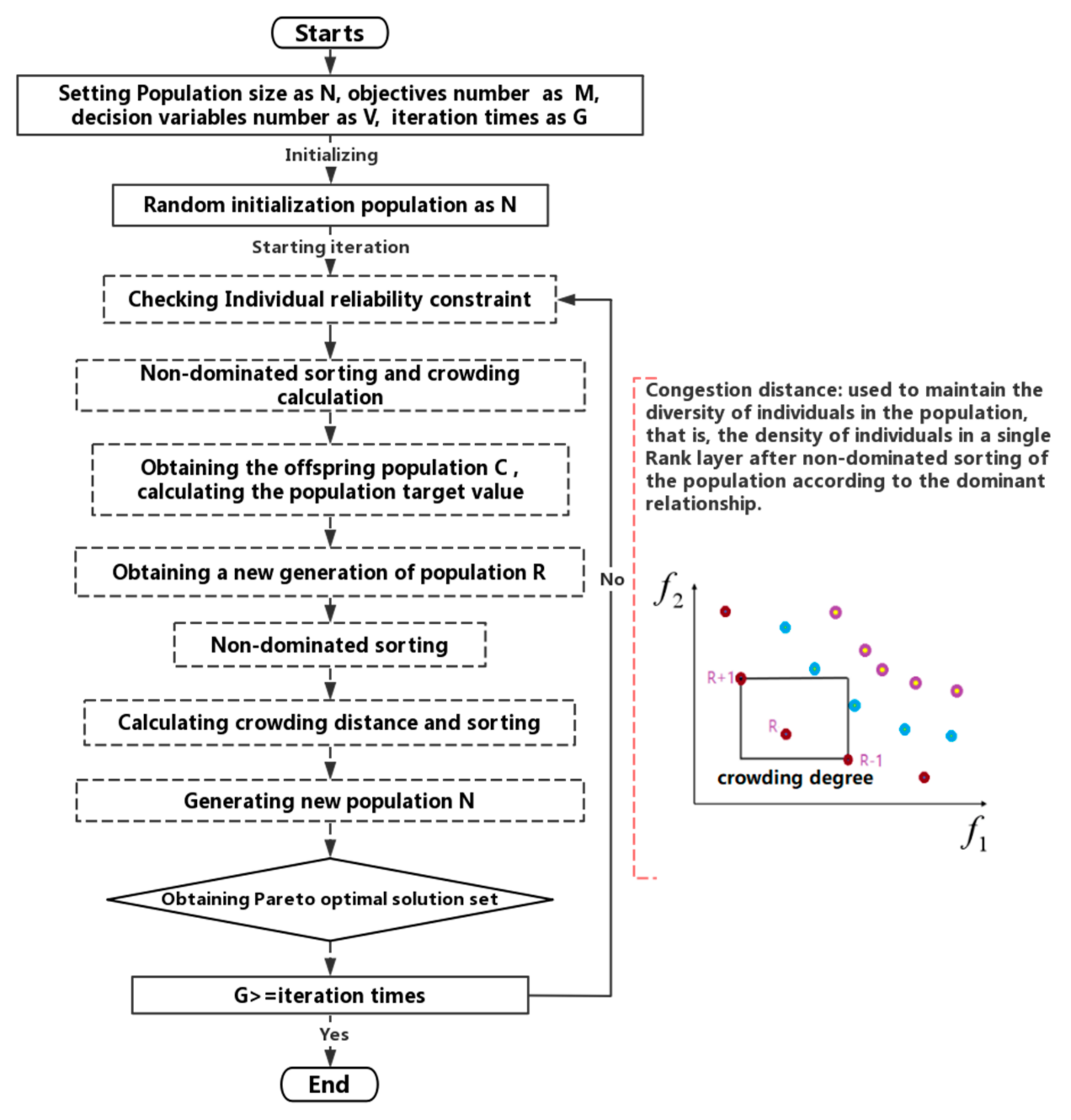
2.3.1. NSGA-II

NSGA-II is applied in many fields, and is one of the most popular multi-objective optimization algorithms in intelligent optimization—an elitist non-dominated sorting genetic algorithm with an elite mechanism. The solution process is shown in Figure 2.

2.3.2. NSGA-III

NSGA-III introduces a reference point selection mechanism to replace the crowding distance in NSGA-II, which enhances the diversity distribution of Pareto solutions so as to retain the non-dominated individuals belonging close to the reference point. The algorithm solution process is shown in Figure 3:

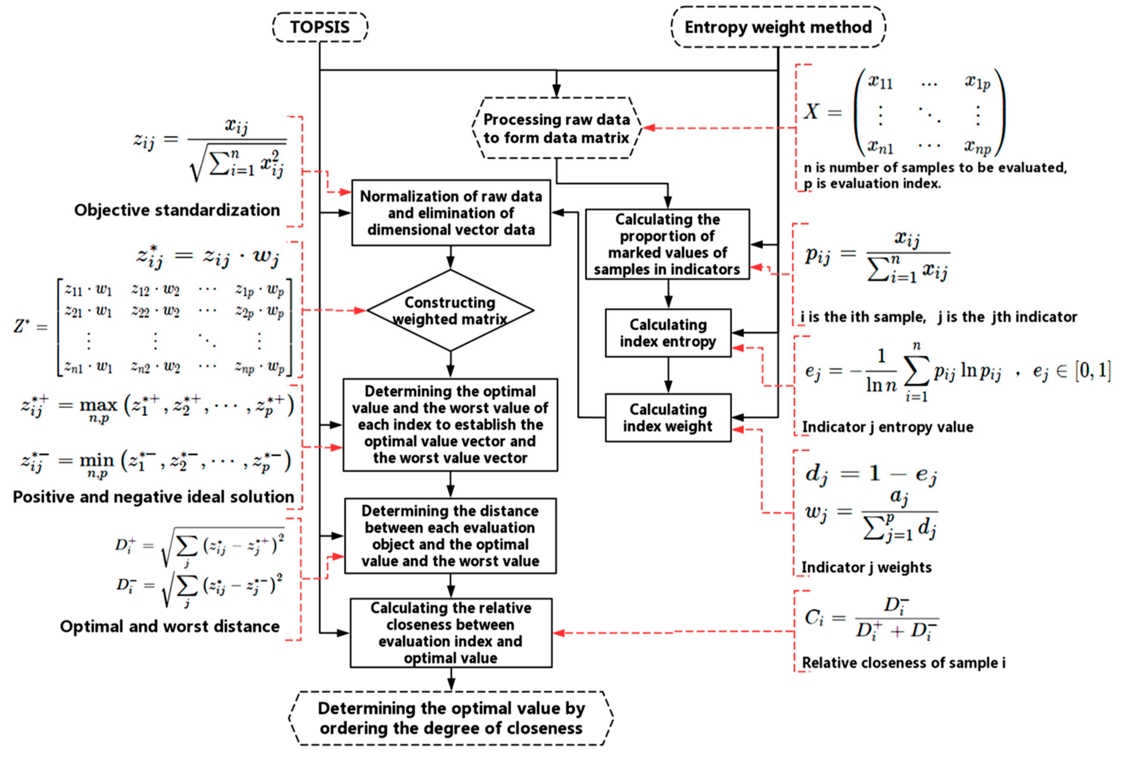
2.3.3. Comprehensive Evaluation of TOPSIS and Entropy Weight

In order to objectively obtain the weight of each objective in the non-dominated solution to determine the optimal solution of optimization, TOPSIS and entropy weight can be combined to conduct comprehensive evaluation by using their respective characteristics.

The solving process is shown in Figure 4:

2.3.4. Quality Evaluation Method of Optimization Solution

Generally, when conducting multi-objective optimization, it is necessary to evaluate the quality of the optimization results of the algorithm, which can be used to compare the performance of different algorithms, or to determine the quality of the solution and the advantages of the algorithm. Common evaluation indexes include generational distance (GD), inverted generational distance (IGD), hypervolume (HV), C-metric, maximum spread (MS), spacing metric (SM), and center distance (CD) [40,41,42]. These indexes have different evaluation criteria to evaluate the convergence and universality of the solution set. Among them, HV is the only known one-dimensional index, and the only known index consistent with the concept of Pareto dominance that can be used to evaluate the comprehensive index of convergence and the diversity of the solution set [43]; it can be used to evaluate the quality of a solution set by the degree of closeness between the solution and the optimal set. The distribution of the solution in the target space will be obtained to some extent [44].

HV is used to evaluate the comprehensive quality of the optimization calculation results in this paper. The larger the HV value, the better the comprehensive performance of the algorithm. The selection of reference points plays a decisive role in the accuracy of HV calculation. When evaluating the same solution set, different calculation results will be obtained with different reference points selected. If A is the Pareto non-dominated solution set, the hypervolume of set A can be expressed as [45,46]:

$$S(A):=\mu (\underset{a\in A}{\cup }\{y\in Y:a_{ref}\prec y\prec a\})$$

(26)

where $\mu$ represents the Lebesgue measure used to measure volume; while $a_{ref}$ represents the reference point.

2.3.5. Objective Normalization

In practical multi-objective optimization problems, the objective function often has different dimensions or units of a different order of magnitude. In order to avoid the singular sample data or the inability to converge in the optimization calculation, it is necessary to convert these objective data into the data with the same dimension or the same order of magnitude, so that they can carry out mathematical operations with one another. The data normalization method—including the linear, logarithmic, and inverse cotangent function method—is often adopted to solve the problem.

(1) Normalization of Objective Function

In this paper, the linear function method is used to transform the target data into the interval dimensionless data as 0 to 1. The normalized expression is:

$$F_i(x)=(f_i(x)-f_{\min }(x))/(f_{\max }(x)-f_{\min }(x))\hspace{1em}\left(i=1,2,3\right)$$

(27)

where $F_i(x)$ is the normalized target value; $f_{\min }(x)$ is the lower limit of target i; and $f_{\max }(x)$ is the upper limit of target i.

(2) Fitness Function

After normalization, it is necessary to construct a fitness function to verify the stability of the normalization model by weighting an objective. The optimization of this section includes three objectives, with each weight as 1/3. Thus, the specific expression is as follows:

$$fitness(x)=(F_1(x)+F_2(x)+F_3(x))/3$$

(28)

3. Optimization Example

3.1. Project Profile

The example selected in this paper is an energy-saving demonstration center swimming pool. The building area is 1143.20 square meters and the building height is 6.61 m. The average pool water depth is 1.2 m. The water length is 30 m from east to west, and 15 m from north to south. The maximum area of the solar photovoltaic panels and flat-panel solar collectors is 372 m², and the maximum capacity of the ground-source heat pump is 200 kW. On the basis of fully considering the actual social and environmental factors—such as the load demand of the swimming pool, the surrounding available energy resource conditions, the local climate characteristics, and the size of the installation site—and through the comparative analysis of the schemes, it is determined that solar energy, geothermal energy, air energy, natural gas, and power grid electricity purchase comprise the energy sources, while photovoltaic panels, flat-panel solar collectors, ground-source heat pumps, air-source heat pumps, gas boilers, batteries, hot water storage tanks, plate heat exchangers, and other equipment are jointly used to meet the electricity load, air conditioning cooling load, air conditioning heat load, and hot water load demands.

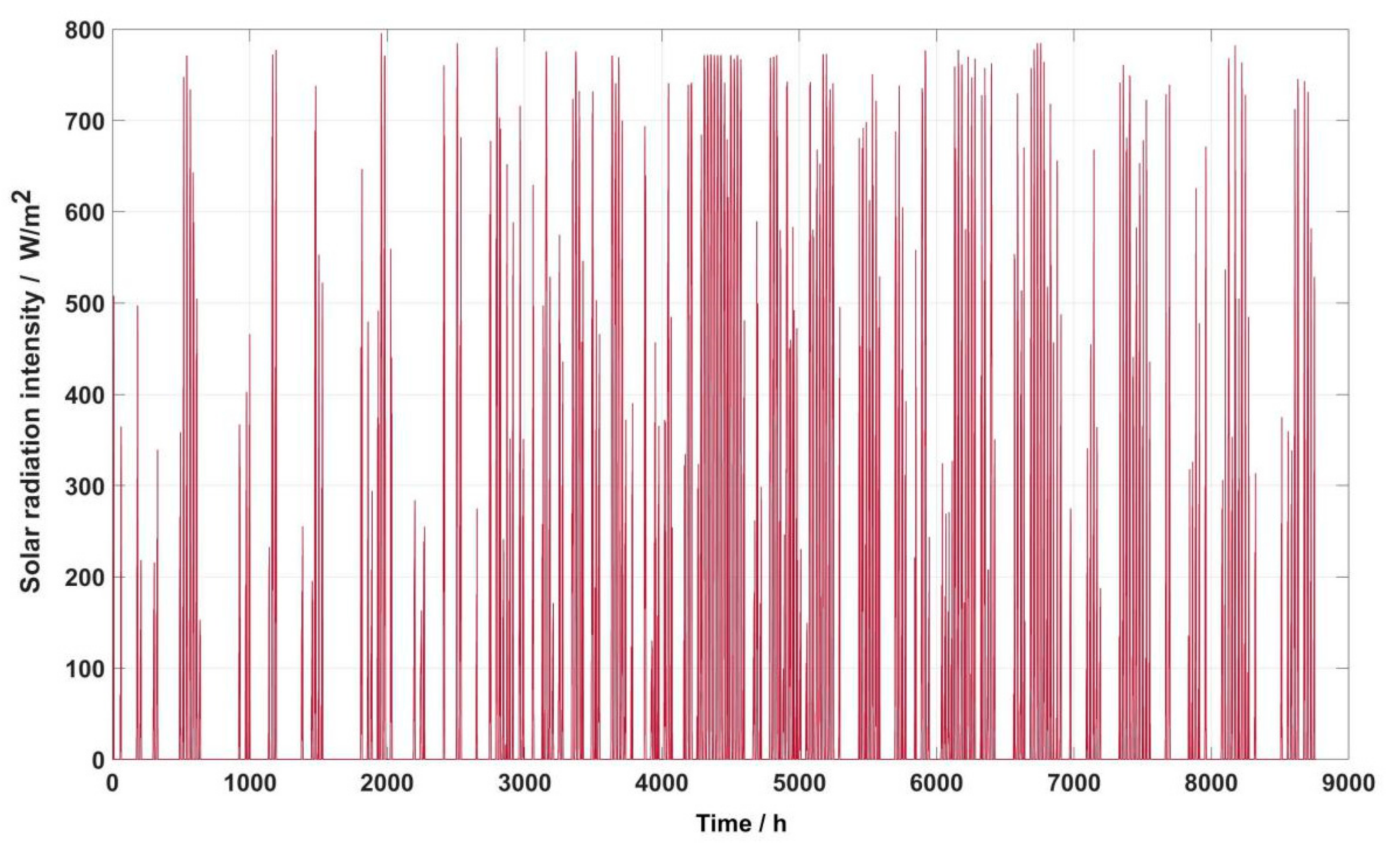
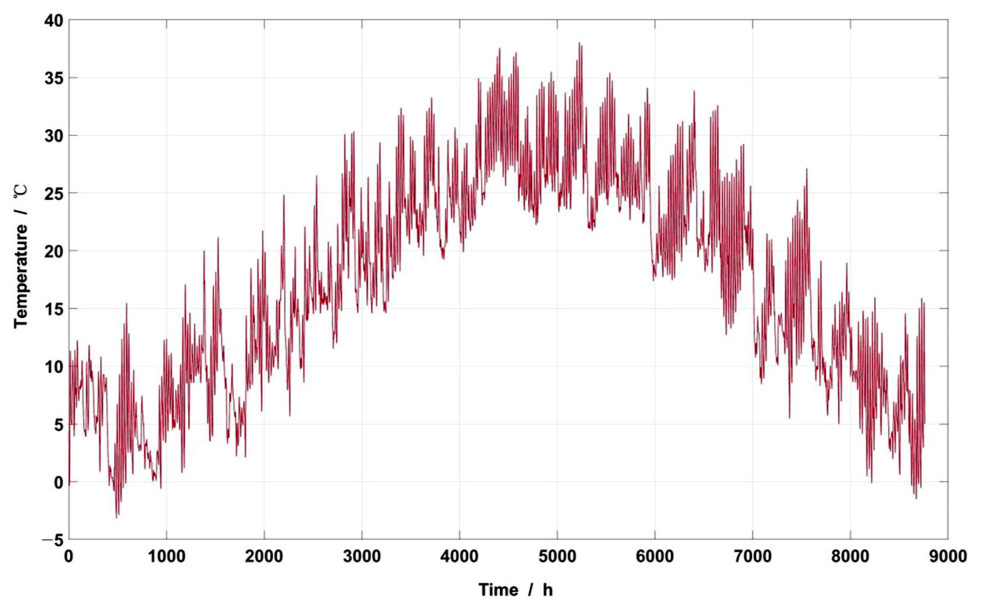
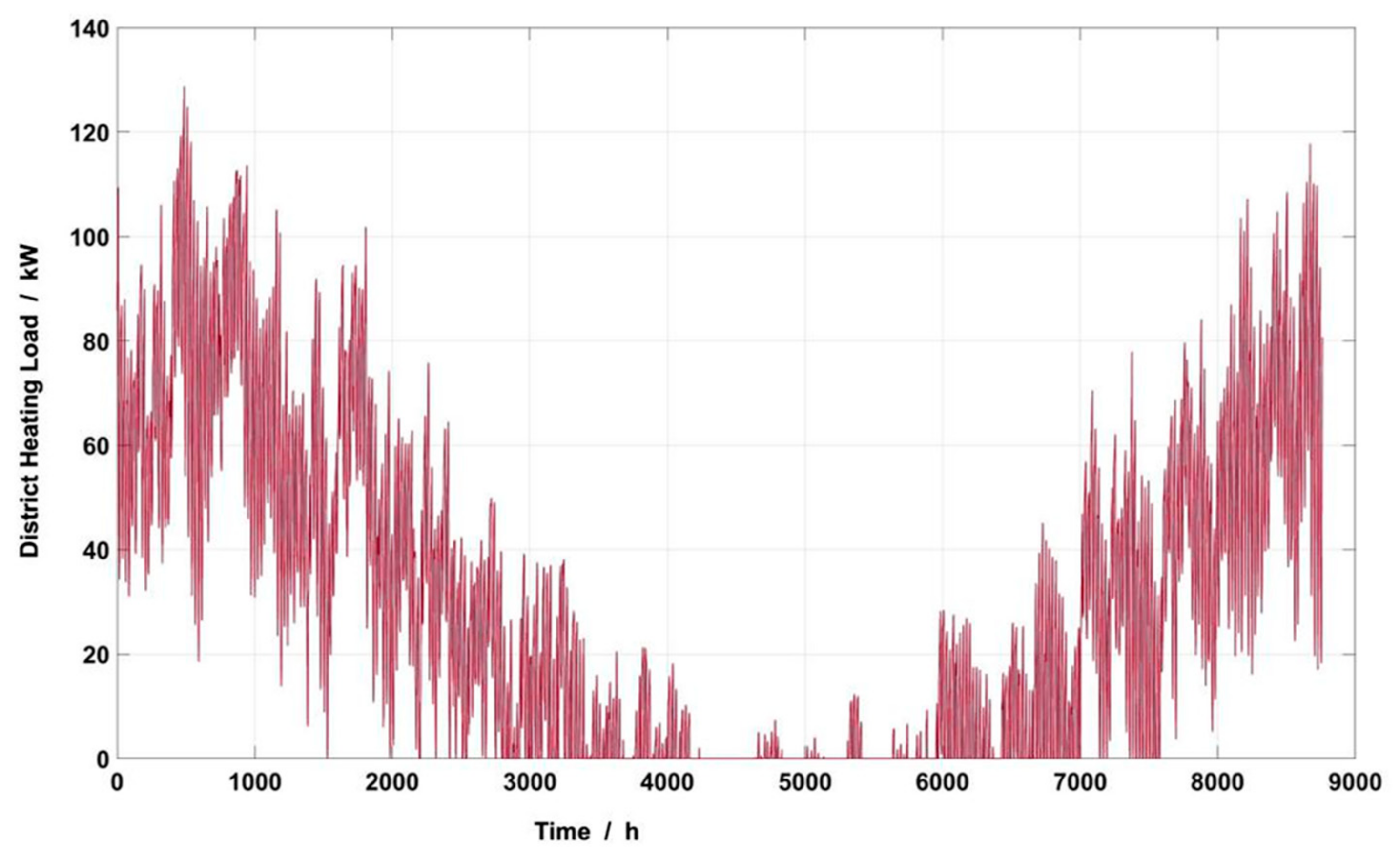
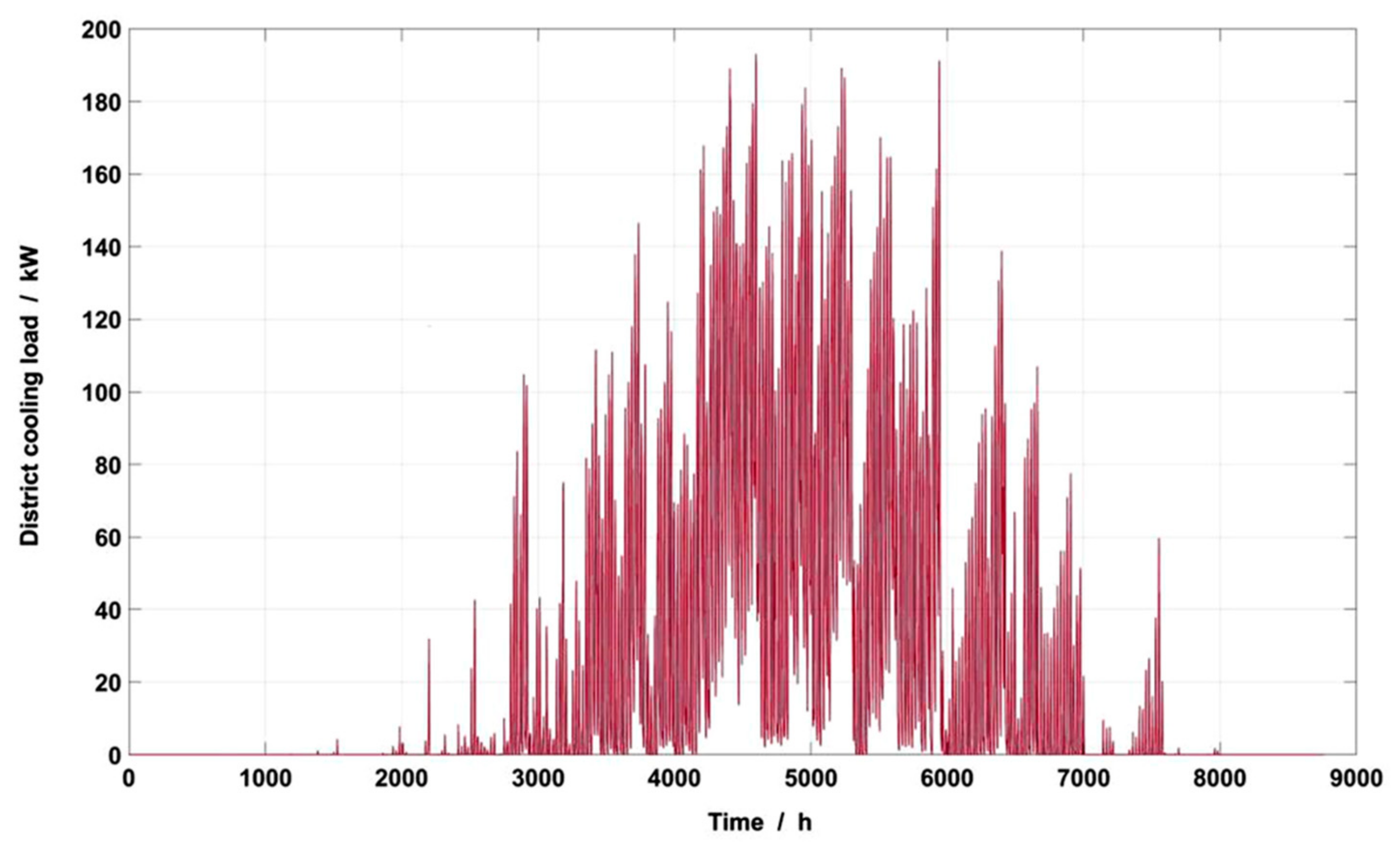
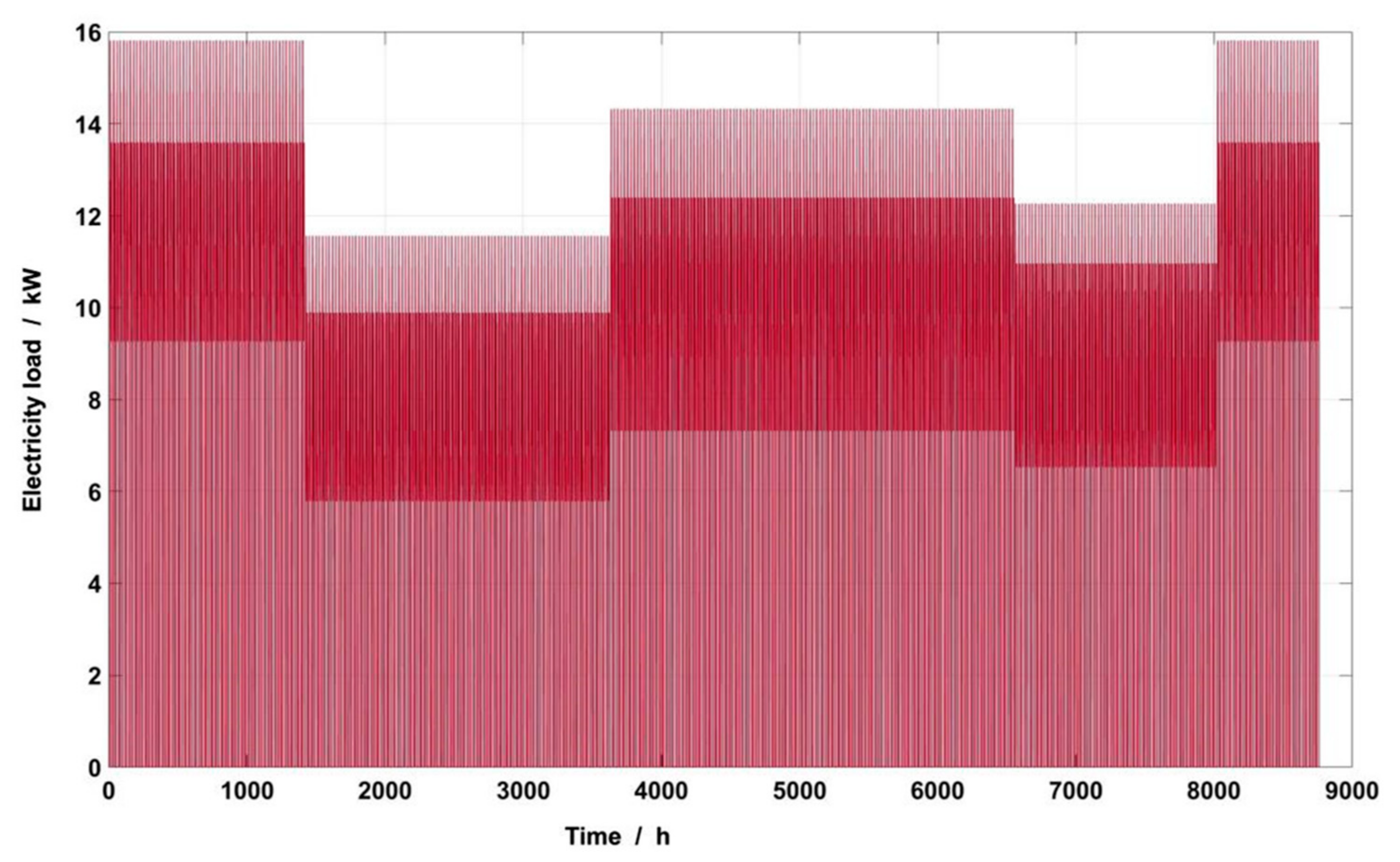
3.2. Meteorological Parameters and Load Demand

The local meteorological conditions need to be considered in the optimization process. Based on the meteorological data released by the National Meteorological Data Network, the annual hourly solar radiation intensity and annual hourly temperature of Changsha City were obtained, as shown in Figure 5 and Figure 6, respectively [47]. It can be shown that the average solar radiation intensity in Changsha is 81 W/m², the annual total sunshine hours are 1636 h, and the solar guarantee rate is ≤ 40%. However, in general, there is a certain level of solar radiation intensity in all seasons, and the total radiation intensity in summer is higher. The annual average temperature is ~17 °C, and the relative temperature is higher in summer and autumn.

Before the optimization work was carried out, the related load of the swimming pool was predicted, and the specific characteristics are shown in Figure 7, Figure 8, Figure 9 and Figure 10. The maximum total cooling load of the swimming pool in summer is 74.40 kW, and the maximum total heat load in winter is 122.80 kW. Due to indoor air conditioning during the pool water heating time, the pool water temperature is effectively considered to be constant. Thus, the load for maintaining the pool water at a constant temperature can be deemed to be stable hourly, with an average value of 94.73 kW.

3.3. Example Computation Parameter

The example analysis is based on the relevant basic data shown in

Table 1. Equipment data.

Equipment	Unit Price (CNY/m2)	Maintenance Cost Coefficient (CNY/kWh)	Life Cycle (Year)
PV	2500	0.015	15.0
GB	900	0.003	20.0
SC	1600	0.03	30.0
GSHP	3000	0.01	20.0
ASHP	1200	0.02	20.0
HE	220	0.002	20.0
ES	1950	0.0026	15.0
HS	1000	0.013	20.0

and

Table 2. Parameters of ES and HS.

Types	Charge Efficiency	Discharge Efficiency	Discharge Rate	Loss Rate	Unit Replacement Cost
Lead storage battery	0.95	0.95	0.2	0.001	200 CNY/kWh
Heat storage tank	0.90	0.90	0.2	0.01	150 CNY/kWh

, which provide the unit price of optional system equipment capacity, maintenance cost coefficient, and equipment life cycle.

The electricity purchase price adopts the peak–valley electricity price, while the gas purchase cost adopts the municipal gas price in Changsha [48,49], as shown in Figure 11.

3.4. Optimization Parameter Setting

3.4.1. Population Number

Before calculating, the relevant optimized parameters need to be set; the first step is population initialization. The individuals in the initial population are the initial values of the optimization, and the selection of these individuals affects the convergence behavior, because if the initial population is improved, the probability of finding the global minimum can be increased, and the variance of the solution can be reduced [50,51]. Therefore, in order to reasonably select the population number, this paper refers to the method described in [52]: through 500 iterations carried out for population sizes of 100, 150, 200, 250, 300, and 350, and the mean values of 30 independent operation experiments taken, the HV index and iteration time of the corresponding population number can be obtained. By comparing the changes in the average HV index and the average iteration time with the population (shown in Figure 12), the population size used in the calculation can be determined.

As can be seen from the diagram, when the example model is optimized, with the increase in the population size, the HV index value shows an upward trend—that is, the greater the population size, the better the quality of the solution. However, with the increase in the population size, the HV may fluctuate slightly. The iteration time increases rapidly with the increase in the population size, and too large a population will lead to too long a running time. Thus, the population size N = 200 was selected to carry out the optimization calculation in this study.

3.4.2. Other Parameters

Through repeated experiments, the number of iterations (G) is finally selected 1200 times by considering the stability of each evaluation index in the iteration process. The probability of population crossover during evolution is 0.9. The probability of population variation during evolution is 0.1. The distribution index of the crossover operator is 20. The distribution index of the mutation operator is 20. Additionally, in order to avoid incomprehension, the upper and lower limits of the decision variables are set. The lower limit is zero for all of them. The sum of the installation area of the photovoltaic panels and solar collectors does not exceed 372 m² due to the limited site. The upper limit of the ground-source heat pump is also set to 200 kW due to the limited site. Taking into account the actual demand, other equipment is set to a large upper limit, according to the calculation needs.

4. Results and Discussions

4.1. Optimization Results of NSGA-II

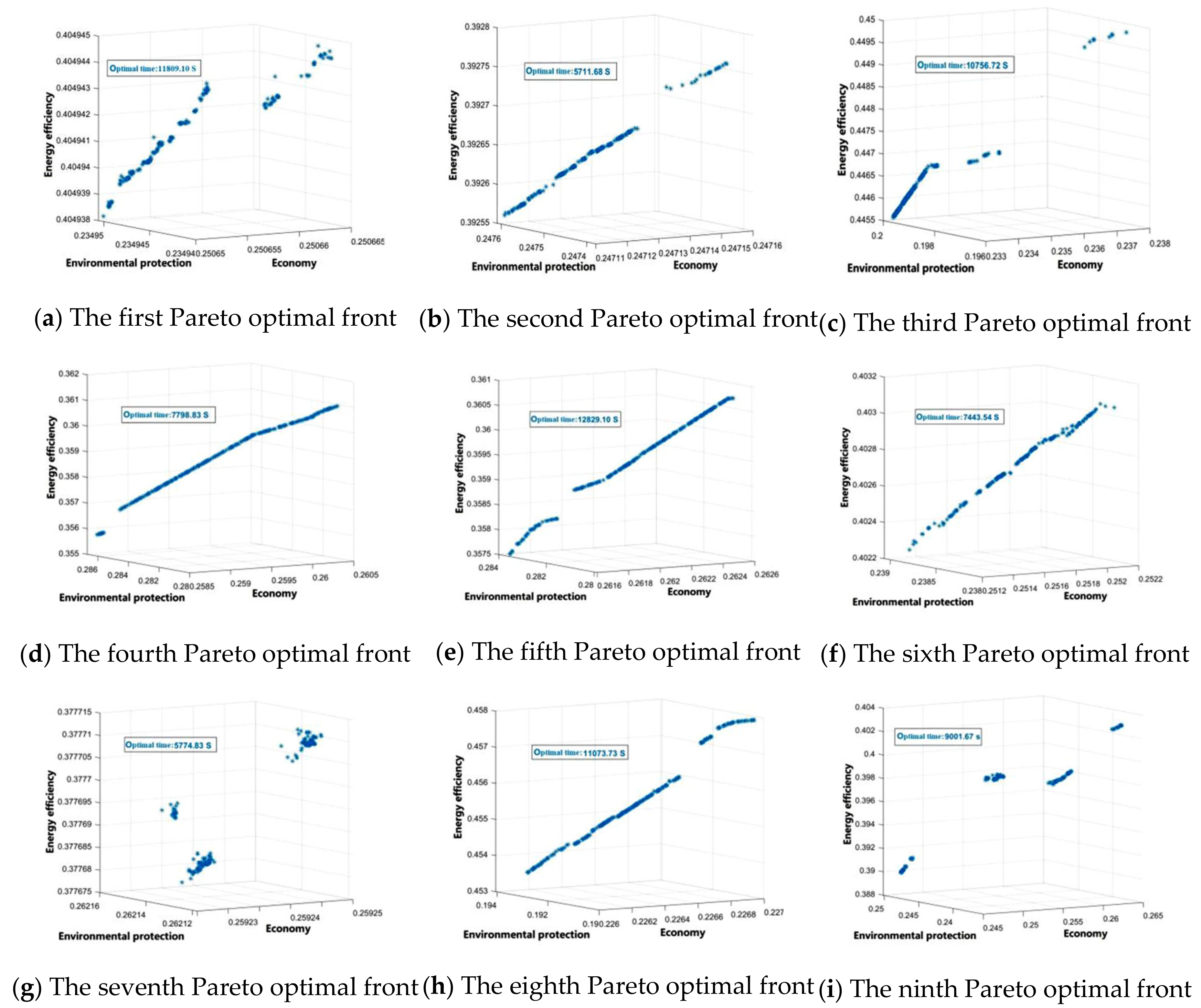
4.1.1. Pareto Optimal Front

A specific initialization method cannot be used by the intelligent optimization algorithm while initializing. Most of the decision variables of the initial population generated by randomness uniformly cover all regions of the search space [53]. Therefore, it is not authoritative to analyze the results only once optimization has been carried out. NSGA-II had to be carried out in 10 independent experiments in the paper in order to provide more reasonable optimization results and minimize the impact of randomness. In view of the layout, only the Pareto optimal fronts obtained from the previous nine optimization calculations were compared, as shown in Figure 13.

It can be seen that the Pareto optimal front distribution, obtained by using the same calculation parameters and models to optimize the example many times, is different for each optimization calculation. First of all, for three-dimensional objectives, the Pareto optimal front is usually a hypersurface, but the three-objective optimization results of the example tend to be close to the three-dimensional curve after many iterations; this is because, in principle, the objectives of intelligent optimization calculation should be mutually contradictory. However, some objectives are not completely contradictory in practice, such as the cost objective and energy efficiency objective in the example, causing the partial degradation of the solution in the optimization process and leading to the Pareto three-dimensional surface forming close to the three-dimensional curve. Secondly, the time consumed in completing 1200 iterations is also very different, which is also caused by the initial population generated by randomness.

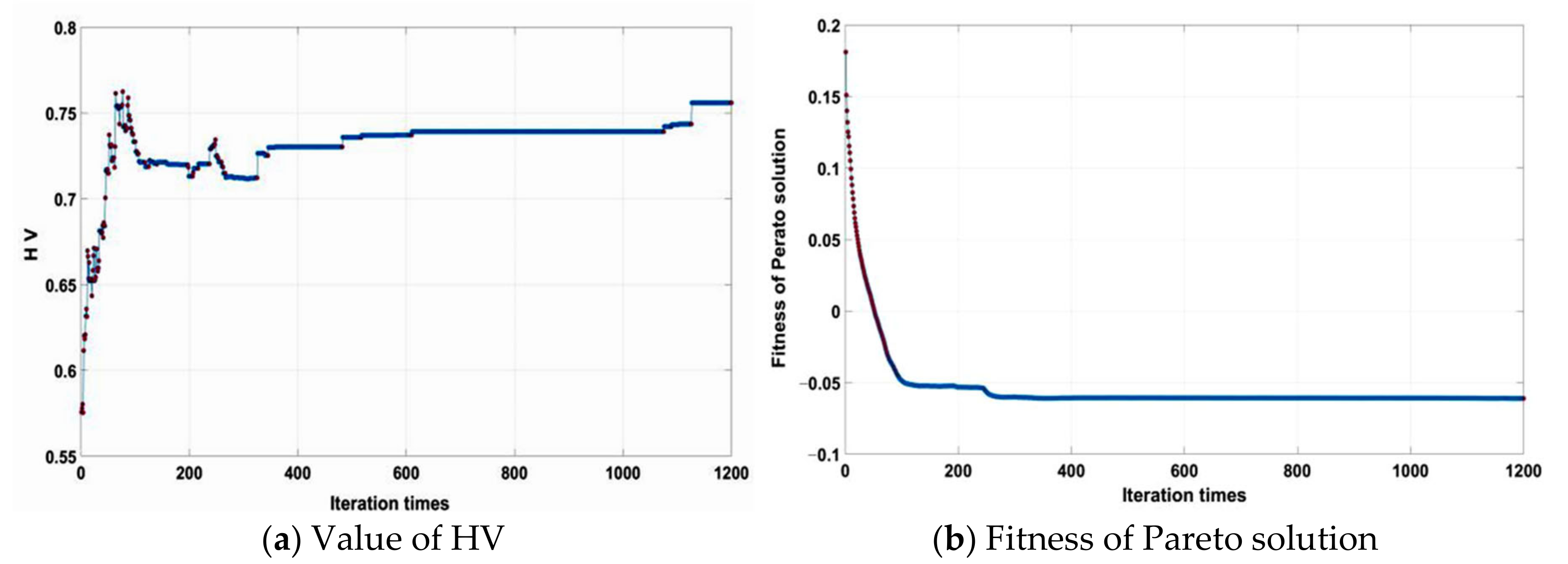
4.1.2. Quality Evaluation of Pareto Solutions

HV index and fitness function are used to evaluate the Pareto solution set of optimization calculations. Based on the optimization results of 10 iterations, the overall trend and value of the two indicators are basically the same. Thus, a group of graphs of evaluation indicators changing with the number of iterations are randomly selected for illustration. The changes in the two indicators are shown in Figure 14. It can be seen that HV increases with the increase in iteration times, and is relatively stable after 800 iterations, which proves that the solution has good quality and uniform distribution. The good convergence of the solution is proved according to the relative stable fitness function after 1000 iterations. NSGA-II can obtain a good optimal solution set when applied to the example in the text.

4.1.3. Objective Weight Analysis

The entropy weight method was used to weight each optimization objective in the Pareto non-dominated solution set of 10 iterations. The weighting results are shown in Figure 15. It can be seen that the relative weight of environmental protection objectives is the largest, with an average of 0.59. The relative weights of economic and energy efficiency objectives are approximated, with average values of 0.21 and 0.20, respectively. Economic goals and environmental goals have the characteristics of a mutual game, and the weight of energy efficiency goals is relatively stable. In practical engineering applications, a certain subjective weighting can be carried out according to the need to participate in decision-making.

4.1.4. Pareto Optimal Solutions

Using a comprehensive decision method with TOPSIS and entropy weight, the Pareto optimal frontiers of 10 iterations were evaluated and sorted in order to determine the Pareto optimal solutions of each optimization, as listed in

Table 3. Pareto optimal solutions of the NSGA-II algorithm for different optimization.

No.	Economy (CNY)	Environment (kg)	Energy Efficiency	HV
1	2,754,550	1,939,800	6.67	0.6072
2	2,730,050	1,989,520	6.50	0.6012
3	2,633,940	1,795,120	7.26	0.6519
4	2,822,240	2,120,480	6.06	0.5744
5	2,837,010	2,119,480	6.06	0.5709
6	2,763,860	1,952,200	6.65	0.6053
7	2,814,680	2,048,480	6.29	0.5822
8	2,588,580	1,761,360	7.41	0.6618
9	2,753,010	1,966,520	6.58	0.6215
10	1,881,010	2,029,160	6.36	0.5927

. The comparison shows that the values of objective function and HV index obtained by each optimization are different, and that the ratios between the maximum and minimum values of the three objectives are 1.5, 1.2, and 1.22, respectively.

4.2. Optimization Results of NSGA-III

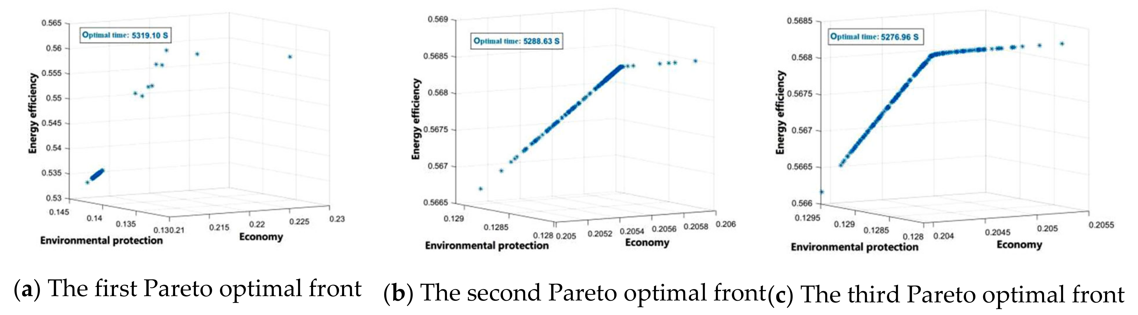
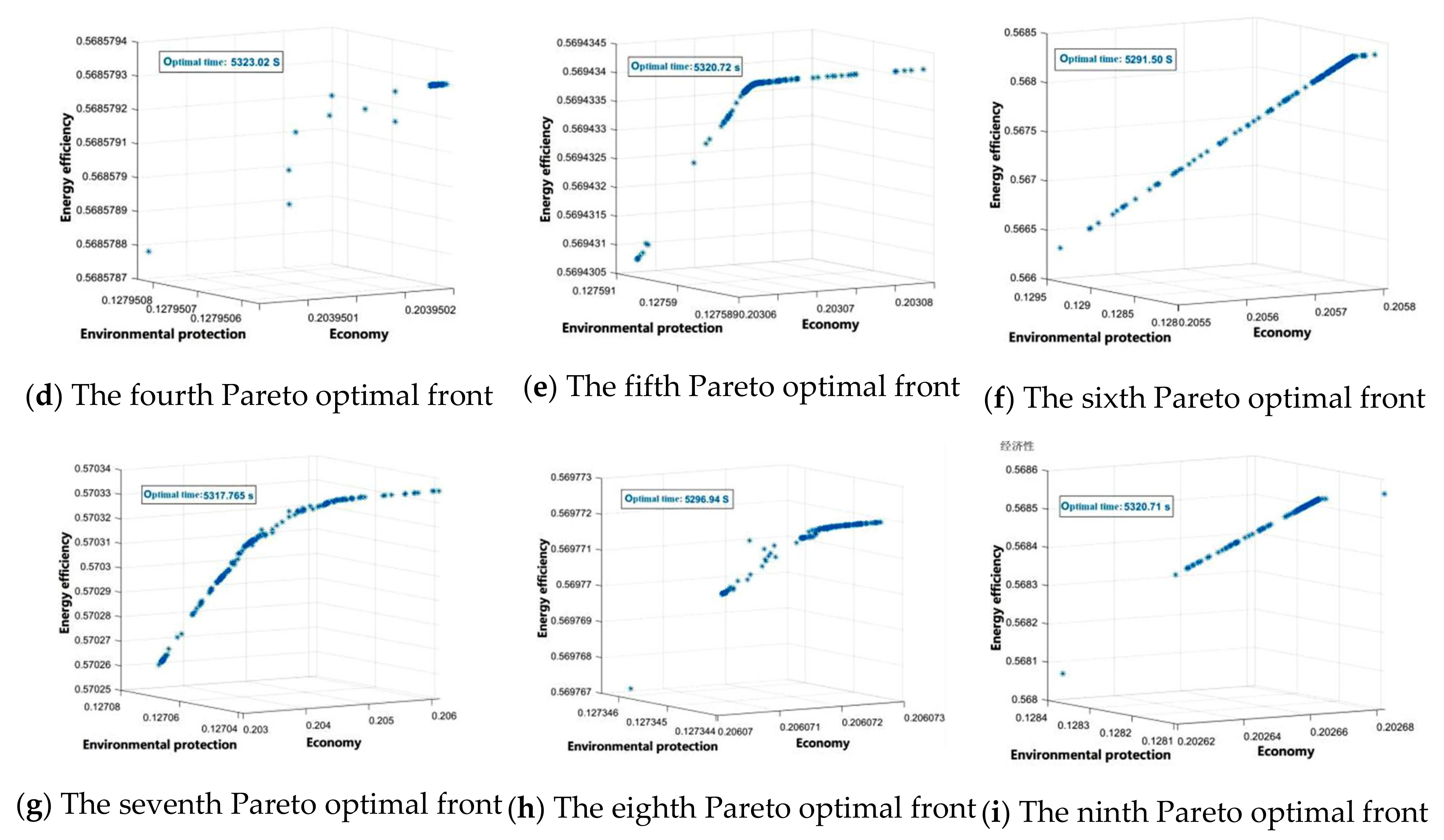
4.2.1. Pareto Optimal Front

Just as with NSGA-II, 10 independent experiments using the NSGA-III algorithm were also conducted, and the Pareto fronts obtained by 9 optimization calculations are shown in Figure 16. Compared with the results of NSGA-II in Figure 13, it can be revealed that NSGA-III also shows different Pareto fronts due to the randomness of initialization, but the stability of the calculation model is relatively good due to the relatively stable optimization calculation time. It should be further explained that the difference between the forward solutions shown in the figure of NSGA-III is greater than that of NSGA-II due to the randomness of initialization. It should be noted that the optimal solution of NSGA-III algorithm is greatly affected by the randomness of initialization, and that the algorithm has better selection ability than the NSGA-II algorithm in this case.

4.2.2. Quality Evaluation of Pareto Solutions

Just as with NSGA-II, the quality of the Pareto solutions for NSGA-III was also evaluated by HV index and fitness function, as shown in Figure 17. The convergence of the solution is proven to be good by the relatively stable fitness function after 800 iterations. Thus, the NSGA-III algorithm can also obtain a better optimal solution set when applied to the example in this study.

4.2.3. Objective Weight Analysis

Figure 18 shows the Pareto solution weighting result of the NSGA-III algorithm. The relative weight of the environmental protection objective is the largest, and its average weight is 0.72. The average weight of the energy efficiency objective is slightly larger than that of the economic objective, with values of 0.18 and 0.10, respectively.

4.2.4. Pareto Optimal Solutions

The Pareto non-dominated solutions of 10 optimization calculations corresponding to NSGA-III were obtained via TOPSIS and entropy weight, as shown in

Table 4. Pareto optimal solutions of the NSGA-III algorithm for different optimizations.

No.	Economy (CNY)	Environment (kg)	Energy Efficiency	HV
1	2,472,380	1,523,400	8.88	0.7559
2	2,437,870	1,511,920	8.96	0.7217
3	2,429,190	1,513,000	8.96	0.7228
4	2,427,650	1,511,800	8.96	0.7198
5	2,495,830	1,517,800	8.92	0.7682
6	2,440,460	1,512,640	8.96	0.7215
7	2,465,870	1,518,840	8.92	0.7627
8	2,442,490	1,059,360	8.98	0.7186
9	2,418,620	1,512,360	8.96	0.7215
10	2,447,740	1,512,440	8.96	0.7175

.

4.3. Comparison of Results and Final Optimization Decision

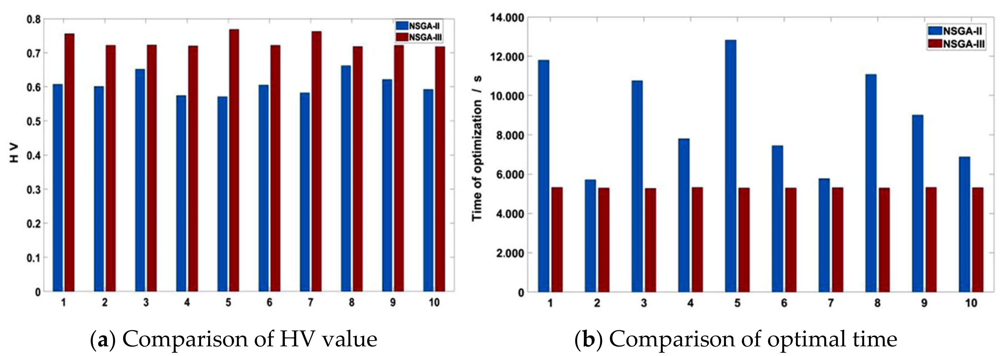
4.3.1. Comparison of Algorithm Performance

The comparisons of HV index and optimization time between the NSGA-II and NSGA-III algorithms after 10 iterations are shown in Figure 19. For the example, the NSGA-III algorithm was better than the NSGA-II algorithm in these two aspects.

4.3.2. Final Decision

The unique optimal solution of the example needs to be obtained through re-decision because it is necessary to obtain the unique solution rather than the solution set in practical engineering applications. The determination of the optimal solution of this example is based on the optimal solution set of 10 independent experiments optimized by the two algorithms, and the optimal solution is determined in three ways: One is to take the average value of the weights corresponding to all of the objectives obtained by the two algorithms in order to obtain the optimal solution. The second is to make a comprehensive decision based on the entropy weight method and TOPSIS on the Pareto optimal solution of the two algorithms after 10 iterations. The third is to use the average method, entropy weight method, and TOPSIS to make a comprehensive decision after combining the optimal solution set of the two algorithms. The re-decision optimal solutions are shown in

Table 5. Optimal solutions and decision schemes.

Methods	Weight Methods	Life Cycle Costs (CNY)	Life Cycle Carbon Emissions (kg)	Energy Efficiency	GB (kW)	PV (m2)	SC (m2)	$\mathit{G}\mathit{S}\mathit{H}{\mathit{P}}_{\mathbf{h}}$ (kW)	$\mathit{G}\mathit{S}\mathit{H}{\mathit{P}}_{\mathbf{c}}$ (kW)	$\mathit{A}\mathit{S}\mathit{H}{\mathit{P}}_{\mathbf{h}}$ (kW)	$\mathit{A}\mathit{S}\mathit{H}{\mathit{P}}_{\mathbf{c}}$ (kW)	HE (kW)	ES (kWh)	HS (kWh)
NSGA-II	Mean value	2,589,580	1,761,360	7.41	101.13	252.42	119.58	200	144.3	33	5.7	776.45	107.48	162.13
	Entropy weight	2,589,580	1,761,360	7.41	101.13	252.42	119.58	200	144.3	33	5.7	776.45	107.48	162.13
NSGA-III	Mean value	2,472,380	152,300	8.88	413.48	371.39	0.6146	199.93	145.41	33.07	4.59	400.28	147.08	51.296
	Entropy weight	2,418,620	1,512,360	8.96	216.19	371.03	0.96546	199.7	145.51	87.49	4.49	283.38	144.36	27.863
Both algorithms combined	Mean value	2,427,650	1,511,800	8.96	199.79	370.4	1.5978	199.87	144.27	33.13	5.73	351.19	148.11	74.859
	Entropy weight	2,472,380	1,523,400	8.88	413.48	371.39	0.6146	199.93	145.41	33.07	4.59	400.28	147.08	51.296

. It can be seen that all solutions of NSGA-III are better than those of NSGA-II. The decision result of NSGA-III with the entropy weight method is better than average. The result of average weighting is better after combining the two algorithms. The economic objective shows the best result in the optimal solution of NSGA-III with the entropy weight method. The carbon emissions show the best result in the average method of solution set union.

The optimization of this example is based on the background form of carbon peak, so the minimum carbon emissions is selected as the final decision-making scheme of the three-objective optimization of the example—that is, the life cycle cost is CNY 2,427,650, the life cycle carbon emissions are 1,511,800 kg, and the primary energy utilization rate of the system life cycle is 8.96. In contrast, in the optimal solution of this group, the capacity of the boiler is moderate. The solar panel is mainly the capacity of the photovoltaic power generation panel, and the solar heat collection is very little. Combined with the energy storage capacity, the scheme intends to rely on renewable energy for power generation, and make full use of energy-storage devices for energy storage and conversion.

4.4. Typical Daily Load Scheduling Strategies in the Example

According to the optimal decision scheme, this section analyzes the load scheduling strategy of each typical day of the example due to the energy balance. Because the building energy supply needs to meet the system load demand, all of the data with energy change in the energy balance diagram below are from 7:00 a.m. to 10:00 p.m. on the basis of the energy characteristics of the swimming pool. The remaining time is non-working time without energy input or output.

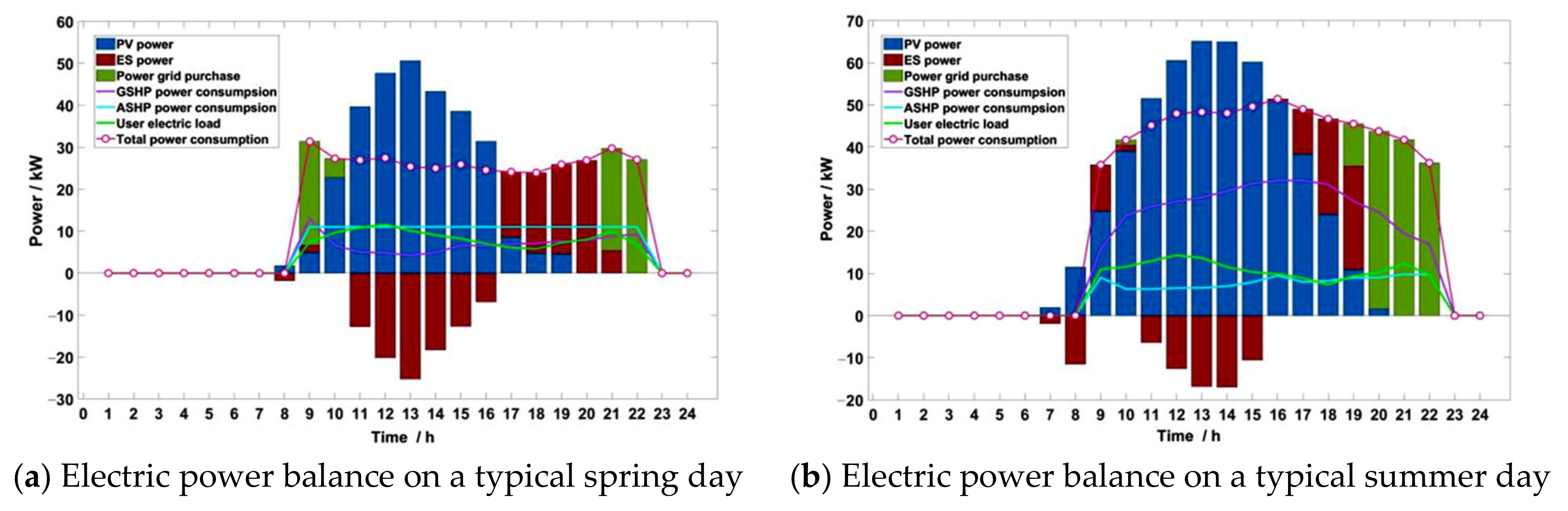
4.4.1. Electric Power Balance

The electric power balance of the four typical days of the example project is shown in Figure 20. Changsha is a hot-summer and cold-winter region, leading to its relatively sufficient light in spring and autumn. Therefore, there is greater photovoltaic output in spring, summer, and autumn, especially from 11:00 a.m. to about 3:00 or 4:00 p.m., when the unconsumed photovoltaic output is stored by the electric energy-storage device. After 5:00 or 6:00 p.m., the photovoltaic output is insufficient or nil; at this time, the energy storage is discharged. The external power grid is enabled to purchase electricity when the energy storage cannot meet the load demand. In winter, due to less light, photovoltaic power supply is short of demand, and there is almost no energy storage, so MCDES energy consumption mainly purchases external power. Overall, more than 70% of the electricity in the four seasons is provided by renewable photovoltaic power generation, and the renewable energy and fossil energy are relatively high primary energy utilization, reflecting the system’s good low-carbon economic behavior.

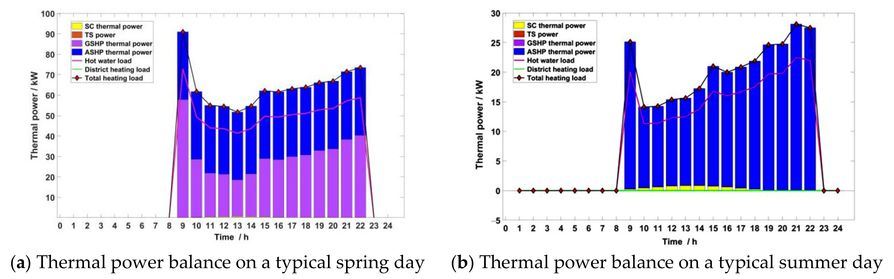
4.4.2. Thermal Power Balance

The thermal power balance of the four typical days of the example project is shown in Figure 21. The heat energy demand includes hot water load and air conditioning heat load. Air conditioning heat load is not required in any season except for winter. The hot water load needs to be met in all four seasons, and the water temperature requirements are constant. The boiler only bears the impact load when the swimming pool is opened. The operation stage is dominated by renewable energy utilization; thus, at this time, there is no natural gas consumption due to the boiler having no output. Therefore, the multi-energy comprehensive utilization of the system shows good low-carbon performance in the operation stage. From the figure, it can be seen that the heating power of the flat-plate solar collector in all four seasons is very small, and can be practically ignored, such that solar heating equipment can be ignored in system planning. Although generally the heat load rate of the ASHP is lower than the heat load rate of the GSHP, the air-source heat pump shows good heat output performance in spring, summer, and autumn due to these three seasons having higher outdoor temperatures in Changsha City. In addition to meeting the demand of swimming pool hot water load, the system should also meet the demand of air conditioning heat load in winter. At this stage, the heat energy is mainly generated by the ground-source heat pump and supplemented by the air-source heat pump because of the low outdoor air temperature. There is almost no thermal energy storage in this scheme due to the thermal energy of the system being mainly based on equipment that consumes electric energy.

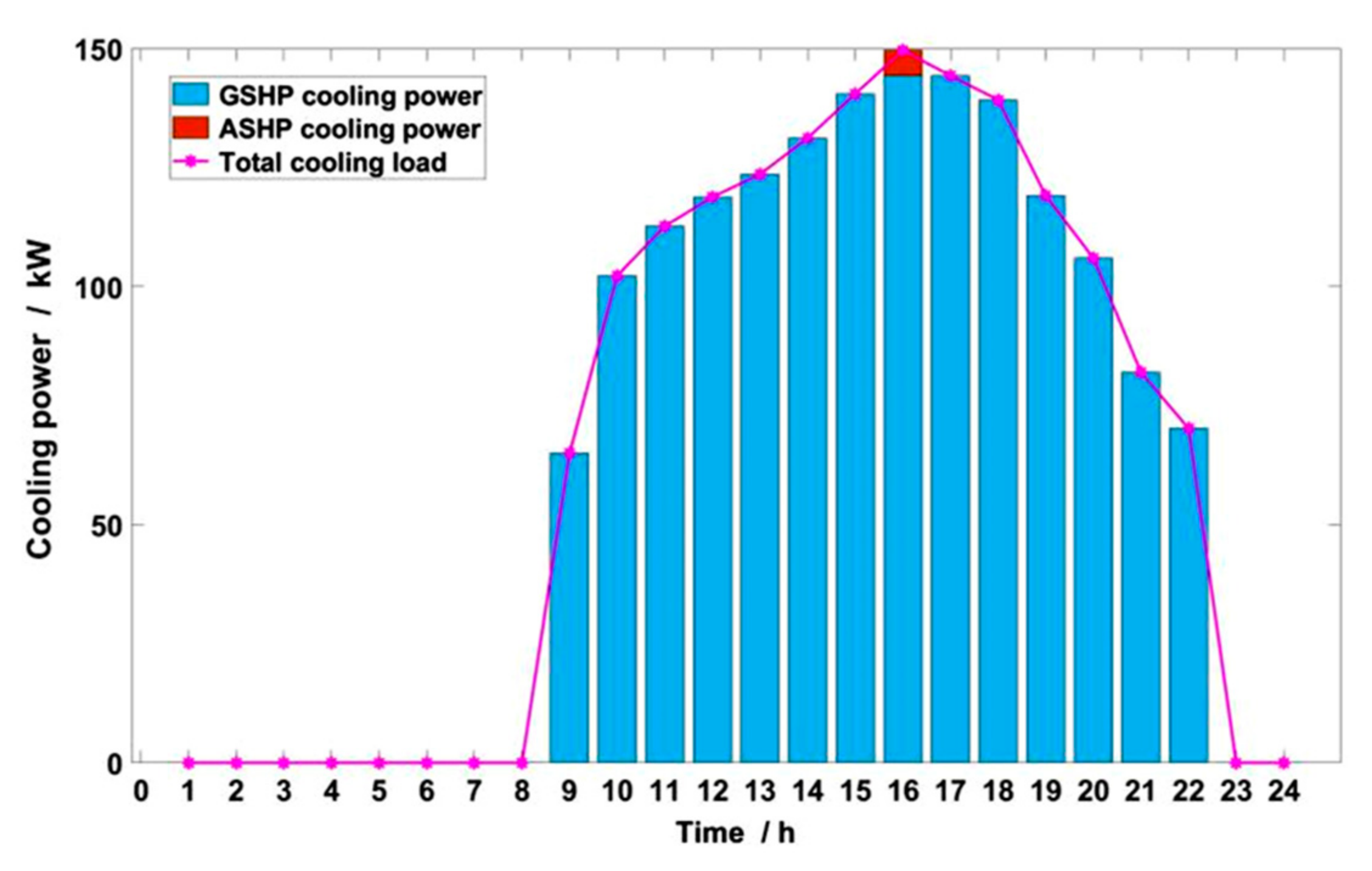
4.4.3. Cooling Power Balance

The swimming pool buildings only have a demand for air conditioning cooling supply in summer, and the cooling power balance on a typical day is shown in Figure 22. The surface temperature is much lower than the ambient temperature while the outdoor air temperature is higher in summer. Therefore, the GSHP is the main cold-supply equipment, and the air source cooling capacity is so small as to be safely neglected.

4.5. Final Decision Scheme of the Example

In practical engineering, the installation area of photovoltaic panels and flat-panel solar collectors in the example swimming pool is limited by the site, which cannot exceed 372 m². The installation capacity of the ground-source heat pump cannot exceed 200 kW. Based on the above factors, and combined with the scheduling characteristics of each piece of equipment on each typical day, the optimal final decision scheme of the example is determined considering the demand of high renewable energy penetration. The boiler is only used to meet the impact load of swimming pool water, so it is taken with the calculated value. Because the output of the flat-panel solar collectors and thermal energy storage is very small, the example eventually does not consider these two devices. In order to make full use of renewable energy, the photo-voltaic panels and ground-source heat pump take their maximum. Since the cooling capacity of the air-source heat pump is very small, its cooling power decision is set to 0. Other equipment is integrated according to the decision value under the optimal solution, based on the optimal solution and energy balance analysis. The final planning of the example is listed in

Table 6. Final decision scheme of the example.

Life Cycle Cost (CNY)	Life Cycle Carbon Emissions (kg)	Energy Efficiency	GB (kW)	PV (m2)	SC (m2)	$\mathit{G}\mathit{S}\mathit{H}{\mathit{P}}_{\mathbf{h}}$ (kW)	$\mathit{G}\mathit{S}\mathit{H}{\mathit{P}}_{\mathbf{c}}$ (kW)	$\mathit{A}\mathit{S}\mathit{H}{\mathit{P}}_{\mathbf{h}}$ (kW)	$\mathit{A}\mathit{S}\mathit{H}{\mathit{P}}_{\mathbf{c}}$ (kW)	HE (kW)	ES (kWh)	HS (kWh)
2,412,200	1,507,300	8.99	200	372	0	200	145	33	5	352	150	0

. Compared with the calculation of the optimal decision scheme, the life cycle cost is reduced by 0.64%, the life cycle carbon emissions are reduced by 0.3%, and the primary energy utilization rate is increased by 0.45%.

5. Conclusions

5.1. Research Conclusions

In order to promote the efficient utilization of energy system resources, low carbon emissions, environmental protection, and the friendly development of economic multi-energy complementary distributed energy systems, taking the construction terminal of an MCDES as the research object, a multi-objective optimization planning model with the lowest system life cycle cost, the minimum life cycle carbon emissions, and the maximum primary energy utilization as the optimization objectives is proposed, which comprehensively considers the economy, environmental protection, and energy efficiency. Furthermore, the model is based on optimized calculations with an example study.

The research shows that, when solving practical problems, the two genetic optimization algorithms—NSGA-II and NSGA-III—used in this paper should fully consider the characteristics of the system. The results of each optimization calculation are different due to the form of random number adopted when initializing the population. In order to obtain ideal optimization results and avoid the uncertainty caused by this randomness, it is necessary to carry out multiple independent running experiments to obtain more Pareto fronts and carry out comprehensive evaluation to determine the optimal solution of the system optimization.

By evaluating the HV index of the two algorithms and the fitness analysis of the non-dominated solution, it can be seen from the quality, uniformity, and convergence of the solution that the two algorithms have good applicability in the optimization model of this paper. Through example calculation, it can be seen by comparing the operation performance of the two algorithms that NSGA-III is superior to NSGA-II in solving the problems studied in this paper. Through the re-weighting and decision-making of the non-dominated solution set obtained via multiple independent runs of each algorithm, the example optimization results were determined as a system life cycle cost of CNY 2,427,650, life cycle carbon emissions of 1,511,800 kg, and a life cycle primary energy utilization rate of 8.96. Based on the analysis of the energy operation strategies of the system under optimal decision-making, it is indicated that the system shows good low-carbon characteristics under the optimal decision-making scheme, which effectively promotes the consumption of MCDES renewable energy, improves and enhances the reliability of the energy supply of the system, strengthens the performance of the comprehensive energy utilization of the system, and verifies the effectiveness and reliability of the optimization model. The energy balance scheduling strategy of the example under the optimal solution policy is analyzed, and the final decision scheme of the example in this paper is determined by considering the actual needs of the project. Under this scheme, the life cycle cost and life cycle carbon emissions are reduced by 0.64% and 0.3%, respectively, compared with those under the optimal solution strategy, while the primary energy utilization rate is increased by 0.45%.

In summary, it is concluded that the study of planning optimization in this paper has a certain social significance, and has a good engineering application reference value for MCDES design optimization.

5.2. Future Works

In future works, the source–load energy supply balance in time and space in the multi-energy system will be considered, and the cascade utilization of energy will be fully considered. In addition, the uncertainty factors of system operation should be considered in order to optimize the MCDES more scientifically and more in line with the actual working conditions, due to the uncertainty factors of the system being further improved with the increase in renewable energy penetration, the changes in real-time electricity price and system operation mode, the random fluctuation of demand-side response, and the opening of the energy consumption market.

References

1. Emara, D.; Ezzat, M.; Abdelaziz, A.Y.; Mahmoud, K.; Lehtonen, M.; Darwish, M.M. Novel Control Strategy for Enhancing Microgrid Operation Connected to Photovoltaic Generation and Energy Storage Systems. Electronics 2021, 10, 1261. [Google Scholar] [CrossRef]
2. Ali, M.N.; Mahmoud, K.; Lehtonen, M.; Darwish, M.M. An Efficient Fuzzy-Logic Based Variable-Step Incremental Conductance MPPT Method for Grid-connected PV Systems. IEEE Access 2021, 9, 26420–26430. [Google Scholar] [CrossRef]
3. Ali, E.S.; El-Sehiemy, R.A.; El-Ela, A.; Adel, A.; Mahmoud, K.; Lehtonen, M.; Darwish, M.M. An Effective Bi-Stage Method for Renewable Energy Sources Integration into Unbalanced Distribution Systems Considering Uncertainty. Processes 2021, 9, 471. [Google Scholar] [CrossRef]
4. Kang, C.; Chen, Q.; Xia, Q. Prospects of Low-Carbon Electricity. Power Syst. Technol. 2009, 33, 1–7. [Google Scholar]
5. Zhu, Q.; Luo, X.; Zhang, B.; Chen, Y. Mathematical modellingm and optimization of alarge-scale combined cooling, heat and power system that incorporates unit changeover and time-ofuse electricity price. Energy Convers. Manag. 2017, 133, 385–398. [Google Scholar] [CrossRef]
6. Sanaye, S.; Khakpaay, N. Simultaneous use of MRM (maximum rectangle method) and optimization methods in determining nominal capacity of gas engines in CCHP(combined cooling, heating and power) systems. Energy 2014, 72, 145–158. [Google Scholar] [CrossRef]
7. Chen, L.; Jia, M.; Huang, Q.; Yuan, X. Modeling and Simulation Analysis of Hybrid AC/DC Distribution Network Based on Flexible DC Interconnection. Power Syst. Technol. 2018, 42, 1410–1416. [Google Scholar] [CrossRef]
8. Lotfi, H.; Khodaei, A. AC versus DC microgrid planning. IEEE Trans. Smart Grid 2017, 8, 296–304. [Google Scholar] [CrossRef]
9. Guo, Y.; Wu, F.; Xu, Q. Optimal capacity allocation strategy for Wind-PV-ES system with different operation modes and its economic analysis considering network loss subsidy. Smart Power 2019, 47, 26–33. [Google Scholar]
10. Qiu, J.; Zhao, J.; Zheng, Y.; Dong, Z.; Dong, Z.Y. Optimal allocation of BESS and MT in a microgrid. IET Gener. Transm. Distrib. 2018, 12, 1988–1997. [Google Scholar] [CrossRef]
11. Chen, C.; Duan, S. Optimal allocation of distributed generation and energy storage system in microgrids. IET Renew. Power Gener. 2014, 8, 581–589. [Google Scholar] [CrossRef] [Green Version]
12. Hou, J.C.; Hu, Q.F.; Tan, Z.F. Multi-objective optimization model of collaborative WP-EV dispatch considering demand response. Electr. Power Autom. Equip. 2016, 36, 22–27. [Google Scholar] [CrossRef]
13. Jing, Y.; Bai, H.; Zhang, J. Multi-objective optimization design and operation strategy analysis of a solar combined cooling heating and power system. Proc. CSEE 2012, 32, 82–87. [Google Scholar] [CrossRef]
14. Mehleri, E.D.; Sarimveis, H.; Markatos, N.C.; Papageorgiou, L.G. A mathematical programming approach for optimal design of distributed energy systems at the neighborhood level. Energy 2012, 44, 96–104. [Google Scholar] [CrossRef]
15. Huang, W.; Zhang, N.; Dong, R.; Liu, Y.; Kang, C. Coordinated Planning of Multiple Enerd Energy Hubs. Proc. CSEE 2018, 38, 5425–5437. [Google Scholar] [CrossRef]
16. Bahramirad, S.; Reder, W.; Khodaei, A. Reliability-constrained optimal sizing of energy storage system in a micro grid. IEEE Trans. Smart Grid 2012, 3, 2056–2062. [Google Scholar] [CrossRef]
17. Jayasekara, S.; Halgamuge, S.K.; Attalage, R.A.; Rajarathne, R. Optimum sizing and tracking of combined cooling heating and power systems for bulk energy consumers. Appl. Energy 2014, 118, 124–134. [Google Scholar] [CrossRef]
18. Salimi, M.; Ghasemi, H.; Adelpour, M.; Vaez-ZAdeh, S. Optimal planning of energy hubs in interconnected energy systems: A case study for natural gas and electricity. IET Gener. Transm. Distrib. 2015, 9, 695–707. [Google Scholar] [CrossRef] [Green Version]
19. Lin, S.; Liu, C.; Li, D.; Fu, Y. Bi-level Multiple Scenarios Collaborative Optimization Configuration of CCHP Regional Multi-microgrid System Considering Power Interaction among Microgrids. Proc. CSEE 2020, 40, 1409–1421. [Google Scholar] [CrossRef]
20. Pelet, X.; Favrat, D.; Leyland, G. Multiobjective optimisation of integrated energy systems for remote communities considering economics and CO2 emissions. Int. J. Therm. Sci. 2005, 44, 1180–1189. [Google Scholar] [CrossRef]
21. Chang, J. Discussion on the key technology of multi-energy complementary, integrated and optimized energy system. Energy Conserv. 2019, 38, 111–112. [Google Scholar]
22. Deb, K.; Srinivas, N. Multi-objective optimization usingnon-dominated sorting in genetic algorithms. Evol. Comput. 1995, 3, 221–248. [Google Scholar] [CrossRef]
23. Deb, K.; Pratap, A.; Agarwal, S.; Meyarivan, T.A.M.T. A fast and elitist multi-objective genetic algorithm: NSGA-II. IEEE Trans. Evol. Comput. 2002, 6, 182–197. [Google Scholar] [CrossRef] [Green Version]
24. Deb, K.; Jain, H. An evolutionary many-objective optimization algorithm using reference-point-based non-dominated sorting approach, part I: Solving problems with box constraints. IEEE Trans. Evol. Comput. 2014, 18, 577–601. [Google Scholar] [CrossRef]
25. Vikram, K.; Ragavendran, U.; Kalita, K.; Ghadai, R.K.; Gao, X.Z. Hybrid Metamodel-NSGA-III-EDAS Based Optimal Design of Thin Film Coatings. Comput. Mater. Contin. 2021, 66, 1771–1784. [Google Scholar] [CrossRef]
26. Tavana, M.; Li, Z.; Mobin, M.; Komaki, M.; Teymourian, E. Ehsan Teymourian. Multi-objective control chart design optimization using NSGA-III and MOPSO enhanced with DEA and TOPSIS. Expert Syst. Appl. 2016, 50, 17–39. [Google Scholar] [CrossRef]
27. Jain, H.; Deb, K. An Evolutionary Many-Objective Optimization Algorithm Using Reference-Point Based Nondominated Sorting Approach, Part II: Handling Constraints and Extending to an Adaptive Approach. IEEE Trans. Evol. Comput. 2014, 18, 602–622. [Google Scholar] [CrossRef]
28. Hisao, I.; Ryo, I.; Yu, S.; Yusuke, N. Performance comparison of NSGA-II and NSGA-III on various many-objective test problems. In Proceedings of the IEEE Congress on Evolutionary Computation (CEC), Vancouver, BC, Canada, 24–29 July 2016; Volume 6, pp. 3045–3052. [Google Scholar] [CrossRef]
29. Ciro, G.C.; Dugardin, F.; Yalaoui, F.; Kelly, R. A NSGA-II and NSGA-III comparison for solving an open shop scheduling problem with resource constraints. IFAC-PapersOnLine 2016, 49, 1272–1277. [Google Scholar] [CrossRef]
30. Yannibelli, V.; Pacini, E.; Monge, D.; Mateos, C.; Rodriguez, G. A Comparative Analysis of NSGA-II and NSGA-III for Autoscaling Parameter Sweep Experiments in the Cloud. Sci. Program. 2020, 2020, 4653204. [Google Scholar] [CrossRef]
31. Kuo, M.; Lu, S.; Tsou, M. Considering carbon emissions in economic dispatch planning for isolated power systems: Acase study of the Tai wan power system. IEEE Trans. Ind. Appl. 2018, 54, 987–997. [Google Scholar] [CrossRef]
32. Wang, J.; Lu, Y.; Yang, Y.; Mao, T. Thermodynamic performance analysis and optimization of a solar-assisted combined cooling, heating and power system. Energy 2016, 115, 49–59. [Google Scholar] [CrossRef]
33. Madonna, F.; Bazzocchi, F. Annual performances of reversible air-to-water heat pumps in small residential buildings. Energy Build. 2013, 65, 299–309. [Google Scholar] [CrossRef]
34. Wang, J.; Sui, J.; Jin, H. An improved operation strategy of combined cooling heating and power system following electrical load. Energy 2015, 85, 654–666. [Google Scholar] [CrossRef]
35. Li, H.; Kang, S.; Yu, Z.; Cai, B.; Zhang, G. A feasible system integrating combined heating and power system with ground-source heat pump. Energy 2014, 74, 240–247. [Google Scholar] [CrossRef]
36. Al-Gabalawy, M.; Mahmoud, K.; Darwish, M.M.; Dawson, J.A.; Lehtonen, M.; Hosny, N.S. Reliable and Robust Observer for Simultaneously Estimating State-of-Charge and State-of-Health of LiFePO4 Batteries. Appl. Sci. 2021, 11, 3609. [Google Scholar] [CrossRef]
37. Zhu, Q. Capacity Optimization for Electrical and Thermal Energy Storage in Multi-Energy Building Energy System. Ph.D. Thesis, Shandong University, Jinan, China, 2018. [Google Scholar]
38. Ren, N.; Wang, Y.; Xu, Z.; Hua, X.; Ding, T.; Bie, Z.; Zhang, X. Component Sizing and Optimal Scheduling for Distributed Multi-Energy System. Power Syst. Technol. 2018, 42, 3504–3512. [Google Scholar] [CrossRef]
39. Wang, L.; Zeng, S.; Huang, X.; He, J. Superstructure Model and Optimization Design of Operation Strategy for Distributed Energy System with Multiple Complementary Energy. J. Eng. Rmal Energy Power 2020, 35, 9–17. [Google Scholar] [CrossRef]
40. Eldhuizen, D.A.V.V.; Lamont, G.B. Multiobjective Evolutionary Algorithm Research: A History and Analysis; Technical Report TR-98-03; Department of Electrical and Computer Engineering, Air Force Institute of Technology: Dayton, OH, USA, 1998; Volume 10. [Google Scholar] [CrossRef]
41. Zhou, A.; Jin, Y.; Zhang, Q.; Sendhoff, B.; Tsang, E. Combining model-based and genetics-based offspring generation for multi-objective optimization using a convergence criterion. In Proceedings of the 2006 IEEE Congress on Evolutionary Computation, Vancouver, BC, Canada, 16–21 July 2006; pp. 892–899. [Google Scholar]
42. While, L.; Hingston, P.; Barone, L.; Huband, S. A faster algorithm for calculating hypervolume. IEEE Trans. Evol. Comput. 2006, 10, 29–38. [Google Scholar] [CrossRef] [Green Version]
43. Zitzler, E. Evolutionary Algorithms for Multiobjective Optimization: Methods and Applications. Ph.D. Thesis, Swiss Federal Institute of Technology, Zurich, Switzerland, 1999. [Google Scholar]
44. Hwang, C.L.; Yoon, K. Multiple Attribute Decision Making: Methods and Applications, A State of the Art Survey; Springer: Berlin, Germany, 1981. [Google Scholar] [CrossRef]
45. Zitzler, E.; Thiele, L.; Laumanns, M.; Fonseca, C.M.; Da Fonseca, V.G. Performance Assessment of Multiobjective Optimizers: An Analysis and Review. IEEE Trans. Evol. Comput. 2003, 7, 117–132. [Google Scholar] [CrossRef] [Green Version]
46. Zhou, X.-L.; Guo, P.; Chen, B.-W. Comparative Research on Algorithms for Computing Hypervolume. Comput. Eng. 2011, 37, 152–157. [Google Scholar] [CrossRef]
47. National Weather Data Center [EB/OL]. Available online: http://data.cma.cn/ (accessed on 5 January 2021).
48. Hunan Province Electricity Rate Price List in 2020 [EB/OL]. Available online: http://m.cs.bendibao.com/news/63055.shtm (accessed on 11 January 2021).
49. Pipeline Gas Charges [EB/OL]. Available online: http://www.cs95158.cn/contents/68/1594.html (accessed on 15 February 2021).
50. Kazimipour, B.; Li, X.; Qin, A.K. A review of population initialization techniques for evolutionary algorithms. In Proceedings of the 2014 IEEE Congress on Evolutionary Computation, Beijing, China, 6–11 July 2014; pp. 2585–2592. [Google Scholar] [CrossRef]
51. Glamsch, J.; Rosnitschek, T.; Rieg, F. Initial population influence on hyper-volume convergence of NSGA-III. Int. J. Simul. Model. 2021, 20, 123–133. [Google Scholar] [CrossRef]
52. Jiang, S.; Zhang, J.; Ong, Y.S.; Zhang, A.N.; Tan, P.S. A Simple and Fast Hypervolume Indicator-Based Multiobjective Evolutionary Algorithm. IEEE Trans. Cybern. 2015, 10, 2202–2213. [Google Scholar] [CrossRef] [PubMed]
53. Deb, K. Multi-Objective Optimization Using Evolutionary Algorithms: An Introduction [EB/OL]. Available online: http://www.iitk.ac.in/kangal/deb.htm (accessed on 10 February 2021).
Figure 1. MCDES energy chain.
Processes 09 01388 g001
Figure 2. Calculation flowchart of NSGA-II.
Processes 09 01388 g002
Figure 3. Calculation flowchart of NSGA-III.
Processes 09 01388 g003
Figure 4. TOPSIS and entropy weight comprehensive decision method.
Processes 09 01388 g004
Figure 5. Annual hourly solar radiation intensity.
Processes 09 01388 g005
Figure 6. Annual hourly outdoor temperature.
Processes 09 01388 g006
Figure 7. Annual hourly air conditioning heat load.
Processes 09 01388 g007
Figure 8. Annual hourly air conditioning cooling load.
Processes 09 01388 g008
Figure 9. Annual hourly hot water load.
Processes 09 01388 g009
Figure 10. Annual hourly electricity load.
Processes 09 01388 g010
Figure 11. Peak–valley electricity price and gas price.
Processes 09 01388 g011
Figure 12. Effects of different population sizes on HV and iteration time.
Processes 09 01388 g012
Figure 13. The Pareto fronts obtained via NSGA-II.
Processes 09 01388 g013
Figure 14. HV index and fitness function change with iteration times.
Processes 09 01388 g014
Figure 15. Objective weight comparison of NSGA-II.
Processes 09 01388 g015
Figure 16. Pareto fronts optimized by the NSGA-III algorithm.
Processes 09 01388 g016aProcesses 09 01388 g016b
Figure 17. HV index and fitness change with iteration times.
Processes 09 01388 g017
Figure 18. Objective weight comparison of NSGA-III.
Processes 09 01388 g018
Figure 19. Performance comparison between NSGA-II and NSGA-III.
Processes 09 01388 g019
Figure 20. Typical daily power balance in the four seasons.
Processes 09 01388 g020aProcesses 09 01388 g020b
Figure 21. Typical daily thermal power balance in the four seasons.
Processes 09 01388 g021aProcesses 09 01388 g021b
Figure 22. Typical daily cooling power balance in summer.
Processes 09 01388 g022