On the Application of ARIMA and LSTM to Predict Order Demand Based on Short Lead Time and On-Time Delivery Requirements

Abstract

Suppliers are adjusting from the order-to-order manufacturing production mode toward demand forecasting. In the meantime, customers have increased demand uncertainty due to their own considerations, such as end-product demand frustration, which leads to suppliers’ inaccurate demand forecasting and inventory wastes. Our research applies ARIMA and LSTM techniques to establish rolling forecast models, which greatly improve accuracy and efficiency of demand and inventory forecasting. The forecast models, developed through historical data, are evaluated and verified by the root mean squares and average absolute error percentages in the actual case application, i.e., the orders of IC trays for semiconductor production plants. The proposed ARIMA and LSTM are superior to the manufacturer’s empirical model prediction results, with LSTM exhibiting enhanced performance in terms of short-term forecasting. The inventory continued to decline significantly after two months of model implementation and application.

1. Introduction

Taiwan’s semiconductor industry has been growing consistently for more than three decades, promoted as the strategic high-tech industrial development. The industry specializes in integrated circuit (IC) design, fabrication and, thus, develops complete IC packaging production from upstream IC wafer materials until downstream IC packaging and testing. As a result, Taiwan has the world’s most comprehensive semiconductor companies with high output values, where production processes, testing equipment, components (e.g., substrates and lead frames), and IC modules are recognized as the global leaders [1].

The rapid growth of cloud-based technologies and applications, with a vast volume of data being collected, have led to the rise of artificial intelligence (AI) and machine learning (ML) adoptions. Further, the Internet of Things (IoT) applications have enabled the real-time big data interactions for intelligent systems and applications, which also increase demands for high-volume server and storage clouds. Since 2020, due to COVID-19 lockdowns, the global demands of information and communication electronics have increased dramatically pushing the supply chain under tremendous stress. The shortage of labors and transportation disruptions change the mode of operations of enterprises, schools, and society in general for remote works, teaching, and home entertainment. The increasing demand for PCs and consumer electronics will further drive the demands for the supply chain. In addition to the growth driven by the residential economy, Taiwan’s IC design industry has gradually moved back to Taiwan to expand its IC carrier capacity due to the effect of the trade war between the U.S. and China, which has prompted end-customers to switch orders and has driven the growth of Taiwan’s IC design output value. Overall, according to the Taiwan Semiconductor Industry Association (TSIA) and the Industrial Technology Research Institute (ITRI), Taiwan’s IC industry output exceeded the USD 100 billion record high for the first time in 2020. Taiwan’s IC industry performed well in 2020 despite the epidemic. ITRI estimates that Taiwan’s IC industry will reach USD 120 billion in output value in 2021, another new record high [2,3].

Taiwan’s IC packaging and testing industry has been booming in recent years, and its total production value is already the world’s largest (global professional packaging and testing industry). Nevertheless, at the same time, facing a complex and challenging industry environment, vicious price-cutting competition among packaging and testing factories, pressure from customers to reduce prices, and facing the severe problem of customers choosing alternative materials (recycling tray) reduce costs. It is undoubtedly a massive impact for an IC tray supplier with a high market share and a large-scale manufacturing plant. Therefore, the company realizes that it needs to grasp the correct market pulse, and its main feature is customer-oriented production. The sales pattern, how to respond to customers’ needs, and grasp the needs of the product market is a significant challenge that companies must face today [4]. The company’s market demand forecasts cannot be known in advance. Therefore, the future demand for products is mainly based on the laws and characteristics of the company’s sales data and using data science methods. Prediction capabilities have become an important decision support system for companies when deciding on production numbers. The decision on the production quantity also affects the scale of the company’s inventory. If it can cope with the changes in market demand, it can reduce the company’s inventory pressure and production and sales risks and improve the quality of customer service and market competitiveness.

This research aims to quickly attract the business community’s attention to demand forecasting technology based on time series under the pressure of global competition, the increasing uncertainty of the economy and customer demand, and the rapid development. Predicting possible future results can assist managers in making demand-oriented decisions under the fierce industry-university competition to achieve better cost control. According to Gartner’s international research organization, companies making decisions based on demand orientation can reduce inventory costs by 15–30% and increase spot availability by 15–30%. According to the sales volume data in the past years, the Plato 80/20 rule is established to take the top five products of the case company to predict the demand volume and further predict future changes, and the next period of high precision forecast value can be obtained as production. This is currently the basis for sales planning. Therefore, this study adopts the traditional time-series method to establish the Autoregressive integrated moving average model (ARIMA) model and the long short-term memory (LSTM) model in the neural network-like method, explores the demand for each product through the sales volume of the top five products over the years, and establishes a forecast model for each product demand to solve the case company inventory. The problem of cost and the applicability of the model is summarized to respond to the rapidly changing world trends and enhance the competitiveness of enterprises.

2. Literature Review

To date, decision-makers have recognized that accurate forecasting can have a significant impact on their work and can make a difference; forecasting has been widely used in a variety of fields to know how to predict uncertain events in the future and to use information that already exists to project an uncertain future [5]. One of these areas is demand forecasting. Demand forecasting is the best decision to provide a company’s future needs [6]. Forecasting, which is one of the fundamental goals of statistical modeling [5], is still imperative in many areas of research and application, including the problem of statistical forecasting of future orders [7], prediction of the performance of hot presses in a multi-effect distillation unit [8], energy demand prediction [9], or tourism demand forecasting [10].

The demand forecasting problem has been studied for many years, and there are numerous forecasting methods and techniques developed as qualitative forecasting methods, time series analysis, and causal methods, as shown in Figure 1 [11]. For example, time series is stated as the use of historical data to analyze future values, and the basic concept of the causal method is to obtain causal relationships from experimental studies of causal relationships and theoretical roles in the discourse, incorporating variables or factors that can affect the forecast into the forecasting model. However, the tray demand is intermittent (or irregular), and the traditional approach’s model performance is not very good. Such a demand is characterized by the absence of time-interval demand and a significant variation in the level of demand for the period in which actual demand occurs [12], and intermittent demand is stochastic with a large proportion of zero values, implying a large variability between non-zero values [13].

The qualitative method mainly relies on managerial experience or technical expert prediction. The Delphi method, for example, emphasizes the principle of anonymity in which all participants express their opinions as individuals without disclosing the identity of each opinion. The principle of iteration: in which the chairman of the meeting publishes the opinions of the participants to other participants. Controlled feedback: in which each round requires participants to answer a pre-designed questionnaire, and analyze the results for the next questionnaire revision and repeat for several rounds. Statistical group response: in which all opinions are counted and analyzed for the next questionnaire revision. Controlled feedback: each round requires participants to answer a pre-designed questionnaire and analyze the results for the next questionnaire revision and repeat the process for several rounds. Statistical group response: all opinions are counted and then consolidated for judgment. Expert consensus: the final goal to reach a consensus of expert opinion [14].

Another group of forecasting methods is quantitative techniques. They are mainly used to describe variables and predict the relationship between variables for future causal inference from a large amount of data by numerical or statistical measurement analysis and based on past historical data. Quantitative methods can be divided into two categories—time series methods and causal methods, where time series methods are distinguished from neural networks and LSTM as well as traditional time series methods (e.g., ARIMA) to measure economic forecasts based on these key variables that are believed to affect the forecast values [15]. Another group of forecasting methods is quantitative techniques. They mainly describe variables and predict the relationship between variables for future causal inference from a large amount of data by numerical or statistical measurement analysis, based on past historical data. Quantitative methods can be divided into two categories—time series methods and causal methods, where time series methods are distinguished from neural networks and LSTM as well as traditional time series methods (e.g., ARIMA) to measure economic forecasts based on these critical variables that are believed to affect the forecast values [15].

Autoregressive integrated moving average model (ARIMA) is a time-series forecasting method proposed by Box and Jenkins [16], also known as the Box–Jenkins model. This time-series forecasting method mainly analyzes past and present data, examines its self-correlation and partial self-correlation functions and other characteristics to identify, estimate, and diagnose the three-stage model construction process, fit the best model, and perform data analysis prediction [17]. ARIMA (p, d, q) is a generalized model of Autoregressive Moving Average that combines. The autoregressive process uses the dependencies between observations; several lagged observations (p) is an autoregressive term, and the Moving Average processes and builds a composite model of the time series. Furthermore, a separate approach considers the dependency between observations and the residual error terms when a moving average model is used for the lagged observations (q). The ARIMA (p, d, q) can be modified for different models according to different time series. The p is the number of self-regression terms, d is the number of times to be differenced before the series stabilizes, and q is the number of moving average terms in which the most suitable model is selected. Numerous multiple models are generated by the changes of p, d, and q. First, the best model must be found to describe this time series. The key to time-series forecasting is to predict future values based on the changing pattern of the time attributes of the existing historical data. The selected model corresponded to the ARIMA (1, 0, 1) was validated by historical demand information under the same conditions. The results obtained prove that the model could be utilized to model and forecast the future demand in this food manufacturing. These results provide reliable decision-making guidelines to managers of this manufacturing [18]. The weather forecasting research proposes an Autoregressive Integrated Moving Average (ARIMA) model to forecast better visibility for the variant value of parameters p, d, q using the grid technique. This experiment showed that ARIMA has the lowest mean square error (MSE) value of 0.00029 and a coefficient of variation value of 0.00315. The more significant number of prediction data in the ARIMA model increases the MSE value [19].

Long short-term memory (LSTM) is a type of feedback neural network, which was developed by Hochreiter and Schmidhuber. LSTM algorithms continue to improve after training so that the internal neurons become operational structure intact, and finally find out the most suitable weight ratio of the right, the output parameters. Thus, its predictions are better than general recursive neural network models when LSTM processes data related to forecasting time series in terms of errors and results. At first, LSTM was widely used in robot control, text recognition and prediction, speech recognition, and protein homology detection. However, due to the advancement of algorithms and the rapid growth of computer equipment in recent years, this type of neural network has also been widely used in predicting stock prices and many derivative financial products such as futures, options, and even housing prices.

Long short-term memory (LSTM) is a type of feedback neural network, which Hochreiter and Schmidhuber developed. LSTM algorithms continue to improve after training so that the internal neurons become operational structure intact, and finally find out the most suitable weight ratio of the right, the output parameters. Thus, its predictions are better than general recursive neural network models when LSTM processes data related to forecasting time series in terms of errors and results. At first, LSTM was widely used in robot control, text recognition and prediction, speech recognition, and protein homology detection. However, due to the advancement of algorithms and the rapid growth of computer equipment in recent years, this type of neural network has also been widely used in predicting stock prices and many derivative financial products, such as futures, options, and even housing prices.

LSTM networks predict future stock price trends based on the price history, alongside technical analysis indicators. A prediction model was built with this purpose, and a series of experiments were executed; their results were analyzed against several metrics to assess if this type of algorithm presents, and improvements compared to other machine learning methods and investment strategies. The results obtained are promising, achieving up to an average accuracy of 55.9% when predicting if the price of a particular stock in the near future [20,21]. The LSTM networks are generated for demand forecasts in supply chain management. The future demand for a particular product is the basis for the respective replenishment systems for final customer demand forecasting and increasing the overall value generated by a supply chain. The accurate prediction of PM2.5 (particulate matter with an aerodynamic diameter of ≤2.5 μm) is very significant in managing human health and the government’s decision-making for environmental management. The proposed method was proved to have improved stability and prediction performance compared to multi-layer perceptron and LSTM models [22].

Based on the above, the forecast model uses historical data to simulate the future price direction concerning past data trends. If the forecast accuracy is high, it can be used to reference future decision-making at this stage. Past studies have also confirmed that it is indeed feasible to use historical demand data to simulate forecasting. This study intends to use traditional time series autoregressive integrated moving average and neural network-like long-term prediction models in the dazzling array of new forecasting models. As a research model, long short-term memory is expected to process non-qualitative data, and a predictive model with high accuracy and timeliness can provide ideal research results for this research.

3. IC Factory Scenario and Analysis Framework

This chapter describes the changes in production methods and business models and the pain points faced by enterprises in Section 3.1. Section 3.2—the flow chart of demand in this study is established using existing data; Section 3.3 establishes the traditional time series analysis ARIMA, and LSTM is a set of numbers arranged in chronological order by historical demand quantities. The time is the independent variable, the dependent variable is the relative value of each occurrence of the prediction model, and then the predicted data are compared with the actual data. Finally, Section 3.4 identifies the best forecasting method through the forecasting evaluation metrics.

3.1. Problem Description

In this case, the company is an IC tray material supplier. A small number of diversified companies face the following three difficulties in inventory management at this stage: (1) when the product demand is unstable (such as selecting alternative materials (recycling tray) and tray reuse), the inventory cannot meet the existing demand orders, which can easily lead to overstock or out-of-stock raw materials. (2) When the order fluctuates so much that it is impossible to grasp the delivery time and the scheduled delivery quantity fully, the delivery time is shortened, and the production efficiency is reduced. (3) Due to the wide variety of products, it is difficult and complicated to implement related management. The inaccurate estimation of the empirical model leads to a large inventory of the company. With social progress and the increasing abundance of material products, dominating the market economy has long become customer demand oriented. The rapid development of customized demand makes today’s manufacturing industry adapt to operating in a harsh environment. Customer orders have shifted to a small number of diversified products, causing significant market volatility, and the increase or decrease in the number of product orders changes over time. Therefore, the company cannot respond to the number of goods based on the prior order information and expects to be delivered within the delivery date. However, market fluctuations have caused unstable demand orders. By preparing more inventory, the company can avoid shortages and increase the order completion rate, but it is easy to generate high holding costs. On the contrary, it causes a lack of meetings, resulting in loss of orders and rising costs of out-of-stocks, affecting its reputation. Rapid and diversified market demand has brought changes in business management models due to the drastic changes in modern enterprises’ economic trends and business environments. Enterprises have to reduce inventory risks. In recent years, the visibility of the economy is low, and it is difficult to predict demand. Supply chains must be shortened, making management more difficult. In the industrial age, most manufacturers’ business models mainly use limited data and market information to predict the demand for products as a reference for decision-making and build production capacity to meet order demand and increase capacity utilization, while satisfying customer demands to enhance corporate competitiveness [23].

The flow of demand prediction in this study is shown in Figure 2. First, the data timeline is filtered, and then the missing values and data are removed for regularization.

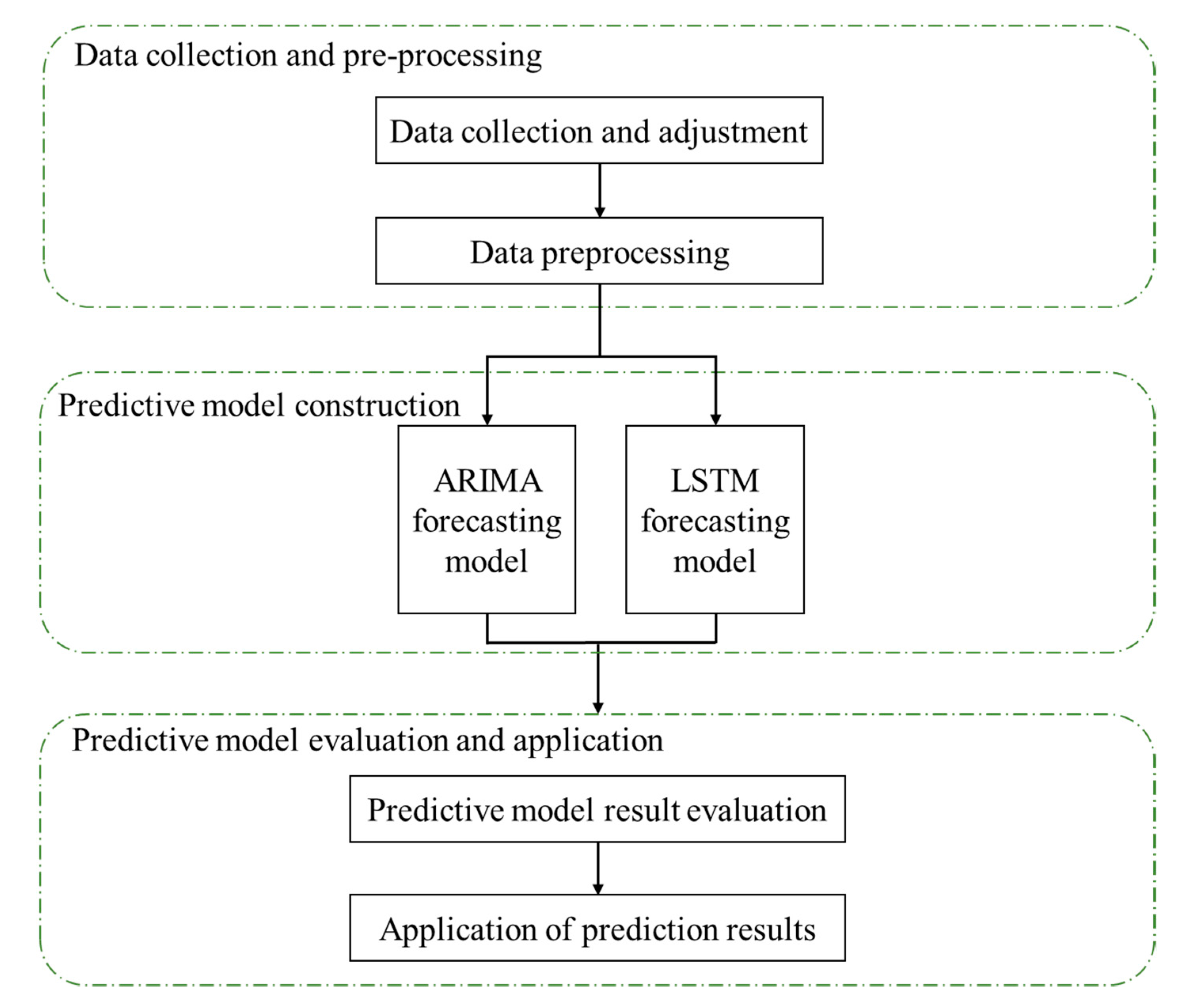
3.2. Data Collection and Adjustment

Case companies collected daily statistics (total of 6000 raw data of sales volume) for this study where the top five sales volumes were documented from 1 January 2017, to 31 August 2019, to find out whether the volume of sales highlighted the season, trend, cycle, empty value, and if the sequence was stable. Therefore, the degree of influence must be based on data mapping and statistical testing before modeling to make a preliminary judgment. The forecast and real data comparison are used to carry out subsequent prediction model data correction and parameter matching. Moreover, the error means square root and average absolute pen error are used to determine the accuracy of the forecast value. The following are the case companies with more than two years of information on Category A products; every month there are orders, and the sales volume of the top five total output products is converted from the day calculation to the cycle; blue is the original material and yellow is the data converted to the cycle.

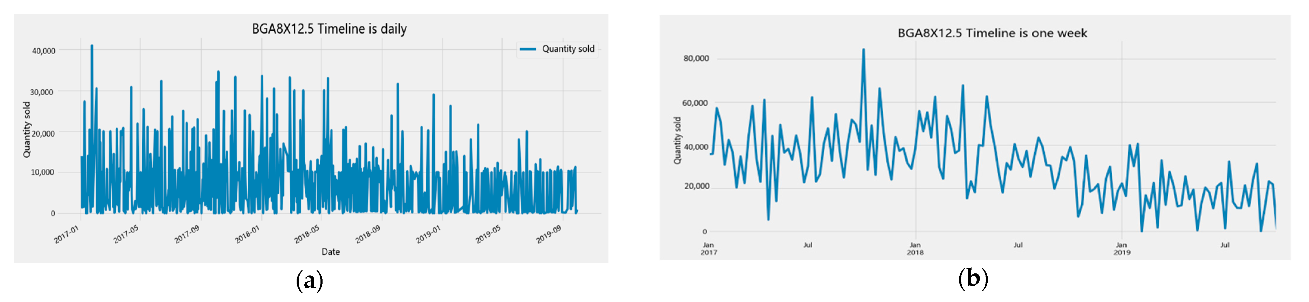
• Timeline conversion: the case companies provide data on the number of goods sold in “days,” and the frequency is converted to the “week” period data. There is no trend and seasonal information for the company’s top five products, as shown in Figure 3. Due to high order volatility, short lead times, and workweek considerations, the prediction horizon is to make short-term sales volume forecasts for the next three weeks. The purpose is to meet customer demand and improve competitiveness with quick response and good forecasting ability. Therefore, this study decided to forecast the periodic data to improve effective management and meet the unstable market demand.

  Figure 3. Timeline conversion of the difference graph. (a) BGA8X 12.5 timeline is daily; (b) BGA8X 12.5 timeline is on week.

  Figure 3. Timeline conversion of the difference graph. (a) BGA8X 12.5 timeline is daily; (b) BGA8X 12.5 timeline is on week.

• Missing value processing.

In this study, converting the original data days into weeks will result in some products not being ordered in a week. Hence, a single week of demand quantity is an empty value, meaning that a value in the existing data are incomplete for subsequent modeling analysis of the following missing value processing methods.

(i)

Remove the missing value.

This method could be the most efficient solution that removes parts of missing values from the analysis sample. However, it also reduces the completeness of data exchange information; discarding hidden information is enough to affect the objectivity and the correctness of results and may lead to poor performance of predictive models.

(ii)

Average interpolation.

This method observes the average instead of the missing value of the observation, and it is simple and easy to use. However, the average interpolation method does not change the overall variable average; the number of variables is small, but when the ratio of missing values is high, the data after insertion changes the overall distribution, forming a high narrow peak distribution.

(iii)

High-frequency data

High-frequency data refers to the short interval between data sampling, and the sampling frequency is greater than the frequency used in the general study, but the concept of high frequency is relative. For example, for stocks, it may take multiple data in a day to be called high-frequency data, and for macroeconomic data, it may be possible to sample once a week can be called high-frequency data. As a result, transaction costs and delays become more critical and degrade API performance when the time scale is smaller with more patterns and samples.

Overall, the sum of a single week is set in the time axis filter. In the process of data conversion, there will be no customer order for a product for a single week, and the value of 0 will be automatically converted during the reading process. The null value is handled by the following four methods of the root mean square error (RMSE) model evaluation, as shown in Figure 4, (a) retaining the original data with an RMSE of 10,176.29; (b) deleting the RMSE of 2072.768; (c) taking the sample on the complementary value of The RMSE of (a) retained original data are 10,176.29; (b) deleted RMSE is 2072.768; (c) up-sampled RMSE is 5222.129; and (d) average RMSE is 7096.927, so the lower RMSE value of the deleted null is chosen to present the historical single-week sales volume data in this study, as shown in Figure 4.

3.3. Model Create and Evaluate

Enterprises face the pain point of changing the mode of production to the business model and use existing data to establish the traditional time-series analysis ARIMA and LSTM in neural network-like methods, in chronological order, by the number of historical demands in a set of numerical order.

3.3.1. ARIMA Model

First, the ARIMA model in this study must establish a stable number of columns. However, the trend of time changes does not necessarily appear in a stable state, so if the original data are not a fixed number of columns, it is necessary to use different methods to change the number of columns into a stable state. It can be called the self-regression integration moving average pattern, also known as the ARIMA (p, d, q) model. ARIMA (p, d, q) can be modified for different models according to different time series, p is the number of self-regression terms, d is the number of times before the sequence is stable, q is the number of moving average terms, which selects the most suitable model. ARIMA (p, d, q) prediction model adjustment steps are as follows:

• Step 1: check whether the data are a steady-state sequence.

Before performing a time-series analysis, it is necessary to determine whether the sequence is stationary. When the sequence data are stationary, the sequence fluctuates around the long-term average value. If the sequence is unstable, the difference is processed by difference. With a steady-state sequence, the integrated order of this variable (Integrated Order) is d, represented by I(d). This study uses AutoCorrelation Function (ACF), Partial AutoCorrelation Function (PACF), and Dickey and Fuller to determine whether the sequence is stationary.

• Step 2: single-root verification determines the number of differences (d).

The primary purpose of the Unit Root Test is to determine the integration level of the time series between variables, to determine whether the time series has reached a steady-state nature. This long-term stable state can be used to carry out future related prediction research. This study uses the ADF test (Augmented Dickey–Fuller test) proposed by Dickey [24] and the single-root test method proposed by the KPSS test because most time series have self-correlation and heterogeneous variations. Therefore, this study adopts the ADF and KPSS [25] verification as a verification-related variable to determine whether the sequence is stationary or not based on the past historical data. The verification model of ADF is as follows.

The original single-root test was the DF single-root test proposed by Dickey and Fuller [24]. It was mainly aimed at the stationary nature of the AR(1) model test sequence, but did not consider that the residual effect may have self-correlation, so Said and Dickey [26] developed the ADF single-root verification method. There are three modes as follows:

Mode 1: no intercept term, no trend

$$\mathsf{∆}{Y}_t=\beta Y_{t-1}+{\displaystyle \sum }_{i=1}^{p-1}{\theta }_i\mathsf{∆}{Y}_{t-i}+{\epsilon }_t$$

(1)

Mode 2: with intercept term, no trend

$$\mathsf{∆}{Y}_t=\alpha +\beta Y_{t-1}+{\displaystyle \sum }_{i=1}^{p-1}{\theta }_i\mathsf{∆}{Y}_{t-i}+{\epsilon }_t$$

(2)

Mode 3: there is an intercept term and a trend

$$\mathsf{∆}{Y}_t=\alpha +\gamma t+\beta Y_{t-1}+{\displaystyle \sum }_{i=1}^{p-1}{\theta }_i\mathsf{∆}{Y}_{t-i}+{\epsilon }_t$$

(3)

where ∆ is the first-order difference, α is the intercept term (intercept or drift term), β is the autoregressive coefficient, t is the time trend term, p is the number of lagging periods in the autoregression, and ${\epsilon }_t$ is the residual term and is subject to the white noise process. The hypothesis test is as follows:

Hypothesis 1.

β = 0 (the sequence is an unsteady sequence, with a single root).

Hypothesis 2.

β$\ne$0 (the sequence is a stationary sequence and does not have a single root).

When the single-root test result does not reject the null hypothesis H1, it means that the sequence is non-stationary and has a single root; when the test result rejects the null hypothesis H1, it means the sequence is stationary does not have a single root.

Although the ADF single-root test does not consider whether there are self-correlation and heterogeneous variation in the residuals, it still has the problem of low-test power. Therefore, in addition to the more common single-root test of ADF, this study adds the KPSS test with different null hypotheses. The most significant difference between the KPSS test and the ADF test is the difference in the null hypothesis. The null hypothesis H1 of the KPSS test is “variable is stationary.” Therefore, H1 does not have a single root. Different verification methods can be used to accurately determine the number of differences between the non-steady-state sequence and the steady-state sequence when performing single-root verification.

The verification model of KPSS is as follows. Kwiatkowski, Phillips, Schmidt, and Shin [25] proposed that the single-root test of the null hypothesis is different from the previous null hypothesis because the variable obeys the steady-state procedure as the null hypothesis. Since most of the single-root tests set the sequence to have a single root, the null hypothesis is the opposite, assuming that the sequence does not have single roots. However, this single-root verification power is not high, and KPSS verification provides a reverse verification method because KPSS verification confirms other single-root verification results.

The KPSS single-root test assumes that the variable is composed of a fixed-term trend, a random walk procedure, and a steady-state white noise:

$$y_t=\xi t+{\mu }_t+{\epsilon }_t$$

(4)

Among them, ${\epsilon }_t$is a steady-state program, $\xi t$ is a random walk,${\mu }_t={\mu }_{t-1}+u_t,{u_t}_{ \sim }^{i.i.d}\mathrm{N}\left(0,{\sigma }_u^2\right)$. At this time, the null hypothesis is H1: ${\sigma }_u^2$ = 0 (or$\xi t$ is a constant), and the opposite hypothesis H1: ${\sigma }_u^2$> 0, the KPSS verification statistics can be derived from the null hypothesis:

$$LM={\displaystyle \sum }_{t=1}^T\frac{S_t^2}{{\widehat{\sigma }}_{\epsilon }^2}$$

(5)

Among them, $S_t^2$ refers to the cumulative sum of residuals, and ${\widehat{\sigma }}_{\epsilon }^2$ is the estimated value of residual variance. The null hypothesis of the KPSS test is H1: ${\sigma }_u^2$ = 0, assuming that the variable is stationary, so the null hypothesis cannot be rejected, which means that the sequence is stationary, which also means that the data have no single root; on the contrary, rejecting the null hypothesis means that the data are non-steady-state, the data should be simplified until it appears steady.

• Step 3: determine the lagging period p and q of ARIMA(p, d, q).

Time-series analysis is mainly based on existing data to predict future changes. In practical applications, time series takes on different forms, and parameters must be sufficient to fit a more suitable model. In 1970, Box–Jenkins methodology proposed The ARMA linear model of the state time series. When the original series has a single root as a non-stationary series, the ARMA model can simplify the parameters of the fitting model. This study uses ACF and PACF as the most basic methods and graphics to initially judge that it is a self-regressive model (Autoregressive model, AR), Moving average model (MA), or auto regression mixed moving average model (auto regression mixed moving average model, ARMA) model reference basis. Tests are often used in practice to avoid errors in human judgments. The trial-and-error method uses parameter estimation to select the smallest AIC and BIC values to fit the best model. In the process of trial and error, limit the order of p and q values to below 3.

ARMA is composed of two “data generating processes.” The time-series model between AR(p) and MA(q) has its characteristics, but the two models must be added together in actual use. There is a high degree of fitness, and the model is as follows:

the generalized model of AR(p) is:

$$y_t={\alpha }_0+{\displaystyle \sum }_{i=1}^p{\alpha }_i{y}_{t-i}+{\epsilon }_t$$

(6)

${\alpha }_0$ is a constant intercept item, p is the number of backward periods, ${\alpha }_i$ is coefficient of $y_{t-i}$, ${\epsilon }_t$ is white noise. AR(p) the model describes a relationship between the current variable and the $y_t$ variable of the last part of the p-period. The generalized model of MA(q) is:

$$y_t={\alpha }_0+{\displaystyle \sum }_{j=1}^q{b}_j{\epsilon }_{t-j}+{\epsilon }_t$$

(7)

${\alpha }_0$ is a constant intercept item, q is the number of backward periods, $b_j$ is the coefficient of${\epsilon }_{t-i}$, ${\epsilon }_t$ is white noise. The MA(q) model describes the relationship between the current variable and the error term effect of the past partial q period. Its economic significance implies the structure of the economic behavior system, which contains the characteristics of “error correction”.

The ACF graph mentioned above measures the decreasing trend between the series index and the positive and negative, i.e., the correlation coefficient of a sequence with its sequence gap k steps is called ACF(k), which determines the order of the MA model.

• Step 4: ARIMA (p, d, q) model selection.

It is imperative to decide the backward period p and q when there is more than one group of ARIMA (p, d, q) in line with the check time. If the backward period choice is too long, it can lead to excessive parameters and inefficient estimated results. On the other hand, if the backward period choice is too short, it can cause oversimplified parameters, resulting in errors in the estimation results. Therefore, it is necessary to select the most appropriate number of backward periods as a forecast model to measure the moderation of the model, determine the appropriateness, and find the optimal number of backward periods. The following two are more commonly used criteria:

Akaike’s information criterion (AIC)

$$\mathrm{AIC}=2k+ln\left(SSE\right)$$

(8)

Bayesian information criterion (BIC)

$$\mathrm{BIC}=N ln\left(SSE\right)+k ln\left(N\right)$$

(9)

where k represents the number of parameters to be estimated in the pattern, N is the total sample number, and SSE is the sum of the squares of the residuals. Choosing the best mode is based on the smaller the AIC and the BIC, the better. In general, small sample data use the AIC to evaluate model matching moderation, while large sample data use the BIC to evaluate model matching moderation.

• Step 5: check that the residuals are white noise.

In a statistical time series, residual analysis is used to examine whether the linear regression hypothesis is met and whether the error is subject to normal distribution. Examining white noise as a random variable in a time series can also be said to understand the assumption that the noise is equal to 0 and the variation is constant, and that it is independent (independently and identically distribute, or iid for short), and the hypothesis is as follows:

Hypothesis 3.

The residuals are subject to white noise.

Hypothesis 4.

The residuals do not obey the white noise.

In this study, the model is detected using the standardized residual graph, normal odds chart, and residual value square graph when diagnosing residuals. If the residual graph falls on the 0-centered line, the residuals of this model are white random processes.

(i)

Standardized residual plot.

Explains that the residuals are randomly distributed with the values in the data sequence chart, and when the sequence does not show patterns, such as trend and periodicity, the residuals can be verified to be independent.

(ii)

Normal quantile–quantile plot.

The main inspection error obeys the normal distribution, divided into formal inspection methods, and graphic judgment. The more commonly used methods are single sample detection (Kolmogorov–Smirnov) and the goodness of fit test (${\mathsf{\chi }}^2$). There is a graphical histogram, but it does not apply when the sample is small). Moreover, box and normal Quantile–Quantile and Q–Q plots) demonstrate the cumulative frequency distribution of the sample and the cumulative rate distribution of the theoretical normal distribution. If the point on the graph is close to a straight line of 45°, it meets the normal allocation assumptions. In this study, the normal odds graph was used to determine whether the residuals met the normal allocation assumptions.

(iii)

Residual histogram.

Checks whether the residuals follow the normal distribution and because the appearance of the histogram changes according to the interval values used to group the data, the normal odds chart is used to evaluate whether the residuals are normal or not.

3.3.2. LSTM Model

LSTM, as an extension of RNN, has a strong capability in forecasting time series data. LSTM can store long-term time-dependent information and the optimal hyperparameters of the LSTM network. The capability of capturing nonlinear patterns in time series data is one of the method’s main advantages, attempting to overcome the challenges of obtaining an accurate forecasting model and considering the intrinsic characteristics of the demand time series (being nonlinear and non-stationary). In the data cleaning, if the sequence contains noisy and missing values, the noise values are smoothed, and the missing values are replaced using appropriate techniques. Applying the proposed methodology to real-time demand data can react appropriately between input and output data and compare to other state-of-the-time series forecasting techniques [27,28]. The prediction steps are described in three steps, where the notations include X (scaling information), + (added information), σ (Sigmoid layer), $h_{t-1}$ (the output of the previous LSTM unit), $C_{t-1}$ (the memory of the previous LSTM unit),$X_t$ (the input), $C_t$ (the latest memory), and $h_t$ (the output).

Step 1:

forget the door (forget unnecessary messages).

Each input has its own weighted LSTM unit, and the sigmoid activation function is between 0 and 1 for nonlinear conversion. The information after the operation is processed by the information ($C_{t-1}$) in the storage memory unit. The product operation controls the information transmission of the previous period in the storage memory unit, obtains the input ($X_t$) of the current period and the output of the previous period (($h_{t-1}$) two vectors), and determines the past output and which parts to delete. For example, when the input is “He has a female friend named Shizuka,” the name of “Nobita” can be forgotten because the subject has become Shizuka. This gate is called the forget gate ($f_t$), and the gate output is ($f_t$) × ($C_{t-1}$).

Step 2:

determine and save the newly input $X_t$ message from the memory unit.

In the sigmoid layer, it was decided to update or ignore those new messages, and according to the tanh layer, input new values to create vectors of all possible values. The input has been updated. This new memory unit is added to the old memory ($C_{t-1}$), and you get $C_t$. In the above example, for the new input, there is a female friend named Shizuka, and Shizuka’s gender has been updated; when the input message is “Shizuka works as a professor at a famous University of Science and Technology in New Taipei City, they recently encountered a classmate meeting.” “Noodle,” at this time words like “famous” and “classmate meeting” can be ignored, while words such as “professor,” “Technology University,” and “New Taipei City” are updated.

Step 3:

determine the output content.

The memory unit generates all possible values through tanh, and the matrix is multiplied by the output of the sigmoid gate. The hyperbolic tangent function non-linearly transforms the updated value and then the dot product operation, representing the value after control calculation whether it can be output smoothly. In the example, if you want to predict blank words, the model knows the “teacher” related nouns in the memory. It can quickly answer “teaching.” It does not directly give the model the answer, but lets it get long-term learning results [17]. The multi-layer LSTM networks method is compared with some well-known time series forecasting techniques from statistical and computational intelligence methods using demand data of a furniture company. These methods include autoregressive integrated moving average (ARIMA), exponential smoothing (ETS), artificial neural network (ANN), K-nearest neighbors (KNN), recurrent neural network (RNN), support vector machines (SVM), and single-layer LSTM. The experimental results indicate that the proposed method is superior to the tested methods in performance measures [27].

In this paper, the product demand forecasts for individual loads, given that the deep neural network LSTM is an effective network to model both the long-term and short-term dependencies in the time series. This model has been proven to have good performance in [29,30].

3.4. Predictive Evaluation Indicators

The common methods to check the accuracy of prediction are MAE (mean absolute error), MAPE (mean absolute percent error), and RMSE (root mean square error), and the smaller the result of the above three calculations, the smaller the prediction error and the better the prediction ability.

(1).

Mean absolute error (MAE): the error between each datum’s predicted and actual value is measured. The MAE method sums up the absolute values of each datum error and then calculates the average error with the following formula:

$$MSE=\frac{1}{k}{\displaystyle \sum }_{t=1}^k{\left(y_t-\overline{f_t}\right)}^2$$

(10)

The average absolute error can obtain an evaluation value, but since it is not known how well the model fits, comparisons are needed to achieve the effect of the evaluation metric.

(2).

Mean absolute percent error (MAPE): MAPE (%) is measured by the relative prediction error of each data to avoid the shortcomings of the MAD method and MSE method, where the calculation results could be too large due to the large data values. When MAPE is less than 10, the model is highly accurate; MAPE is between 10 and 20, the model is a good predictor; MAPE is between 20 and 50, the model is a reasonable predictor and MAPE is greater than 50, the model is not accurate [31].

$$MAPE=\frac{1}{k}{\displaystyle \sum }_{t=1}^k\frac{\left|y_t-\overline{f_t}\right|}{y_t}\times 100\%$$

(11)

(3).

Root mean square error (RMSE): the root mean square error, also known as the standard error, is the square root of the ratio of the square of the deviation of the observed value to the actual value to the number of observations. The root mean square error is used to measure the deviation between the observed and actual values. The standard error is susceptible to very large or very small errors in a set of measurements. Therefore, the standard error is a good indicator of the precision of the measurement. The standard error can be used as a criterion to assess the accuracy of this measurement process, and the formula is as follows:

$$RMSE=\sqrt{MSE}=\sqrt{\frac{1}{k}{\displaystyle \sum }_{t=1}^k{\left(y_t-\overline{f_t}\right)}^2}$$

(12)

where$y_t$ is the actual value,$\overline{f_t}$ is the predicted value, k is the sample size.

The prediction model capability indicators are the three methods mentioned above because MAPE is not affected by the unit and the size of the value, the judgment is based on objective, and the larger the sample size of RMSE, the more reliable the root mean square error. In addition, in this paper, the hybrid formulation proposed here, the residuals from the rolling LSTM model are analyzed for further optimization, given its nonparametric nature and nonlinear predictive ability. An improvement on the metrics would suggest that the residuals are not entirely random and validate the conjecture that macroeconomic predictors can further improve the time-series formulation [32,33]. Therefore, this study uses MAPE and RMSE as the judgment prediction capability indicators.

4. Analysis Results

4.1. Rolling Forecast Structure

The LSTM model in this study has four hidden layers, and the neuron parameters affect the trainable parameters. Furthermore, the output layer defines a neuron used to predict the number of sales, and the training set is divided into 95% of the total data and 5% of the test set. Therefore, the LSTM model often has overfitting during training to make model predictions. For this reason, the in-sample error of this paper uses the loss function (Loss Function) to use the average absolute error (MAE), and the gradient descent method uses Adam optimization. The learning rate is based on the original. Furthermore, the set parameters are 0.02, the epoch is 100, and an epoch of 1 means that all the samples in the training set are trained 100 times, and the batch size is 1. The batch size is the number of samples selected in the training set. Each time a piece of datum are predicted, the initial training value is deleted using the rolling training method. The previous prediction value is added to the training period when the second piece of datum is predicted so that the training length is fixed until the following five test sets are predicted, as shown in Figure 5.

Figure 6 shows the product rolling prediction schematic diagram: the original data are divided into 95% training and 5% test; blue represents the original data, orange is the training data, and green is the test data. Figure 6a shows the results of the 5 predictions using the test set. Figure 6b shows the training length will be fixed; that is, each prediction of datum out, the training set will be deleted from the initial value, and the previous predicted value-added for the training set, predicting the second to fifth data, and so on. Figure 6c is, according to Figure 6b above, the second actual demand quantity to the training set and predict the third to fifth strokes of the test set. Figure 6d adds the third actual demand to the training set and a forecast of the fourth to fifth demand in the test set. Figure 6e adds the fourth actual demand to the training set and a forecast of the fifth demand in the test set.

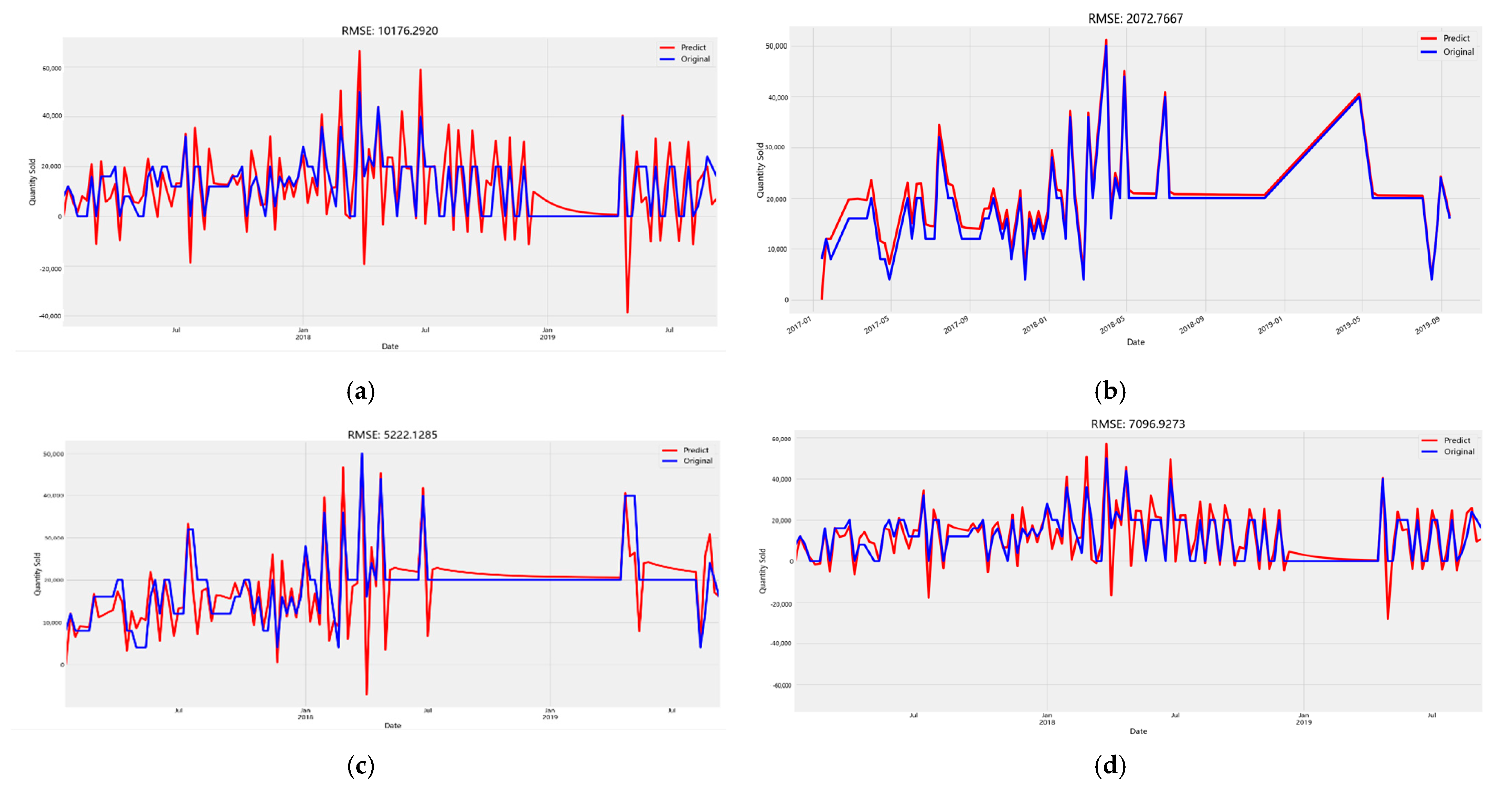
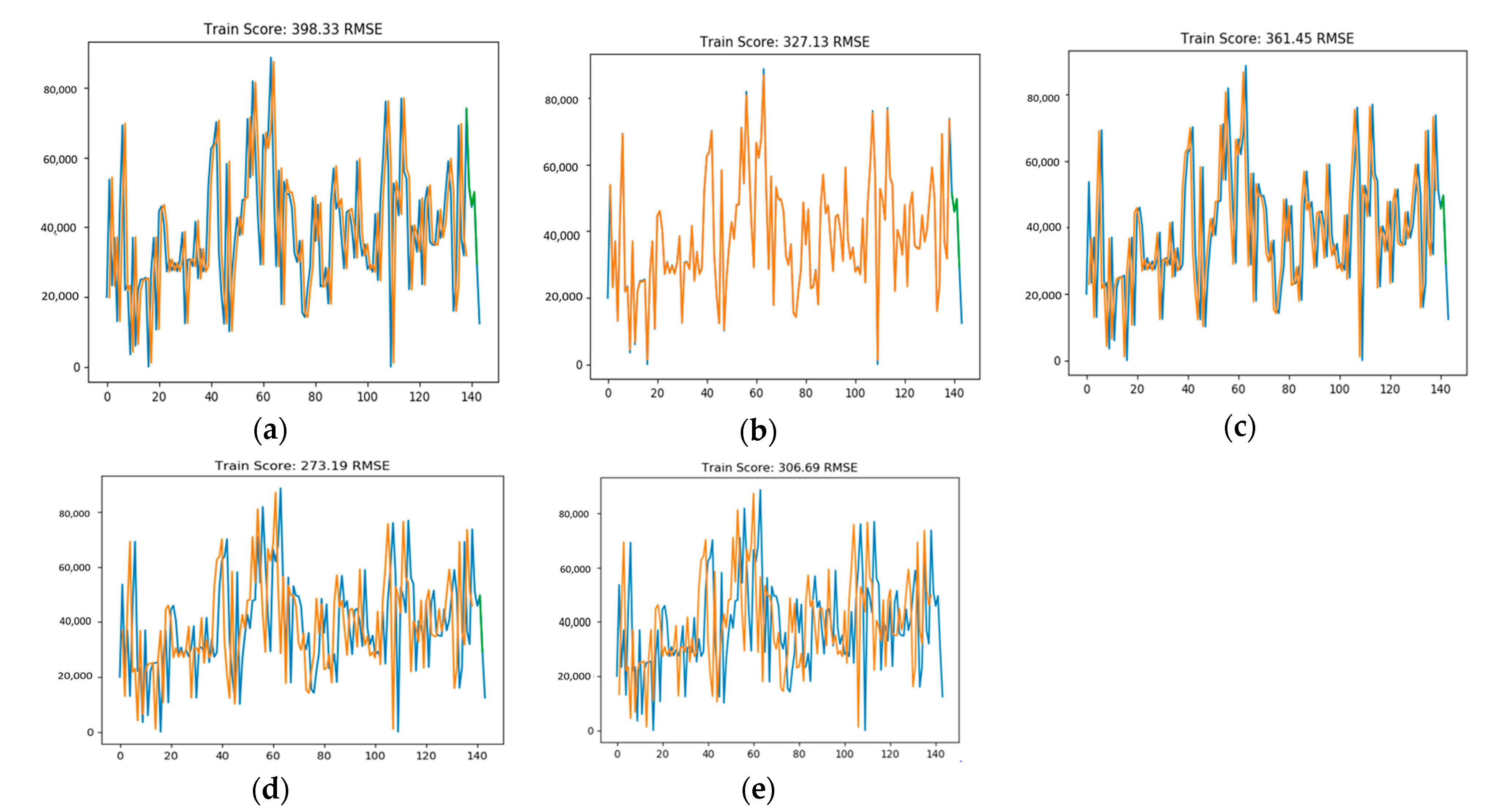
4.2. Model Prediction Results Are Compared

In this study, the IC tray manufacturers provided the data by the industry–academia collaboration. The rule of empirical for the case company is based on the current period moving average forecast. Next, ARIMA and LSTM models were used to forecast the sales volume of the top five products of the case company, and MAPE and RMSE were used as evaluation indicators.

Table 1. Models’ evaluation indicators and comparisons.

Model	Company’s Empirical Law		ARIMA		LSTM
	MAPE (%)	RMSE	MAPE (%)	RMSE	MAPE (%)	RMSE
BGA8X13mm	29.89	19,885.207	6	3507.88	0.2	113.45
BGA8X12.5	3979.29	12,222.978	3015	9108.20	28.3	272.00
TSOP II	1324.73	8954.882	5	1061.47	1.21	293.01
TSOP I	30.00	7689.993	12	5647.35	0.84	116.25
BGA11.5X13	34.20	13,744.552	8	10,273.37	0.62	139.87

shows the analysis results comparing the top five IC trays and finds that both ARIMA and LSTM have more minor prediction errors and significantly outperform the company’s empirical law. For the LSTM prediction results, the minimum and maximum values of RMSE are 113.45 and 293.01, respectively; the minimum and maximum values of MAPE are 0.2 and 28.3, respectively. For the ARIMA prediction results, the minimum and maximum values of RMSE are 1061.47 and 10273.37, respectively; the minimum and maximum values of MAPE are 5 and 3015. The MAPE and RMSE values of LSTM are smaller than ARIMA, which proves that LSTM is more suitable for IC tray prediction than ARIMA.

5. Discussion and Conclusions

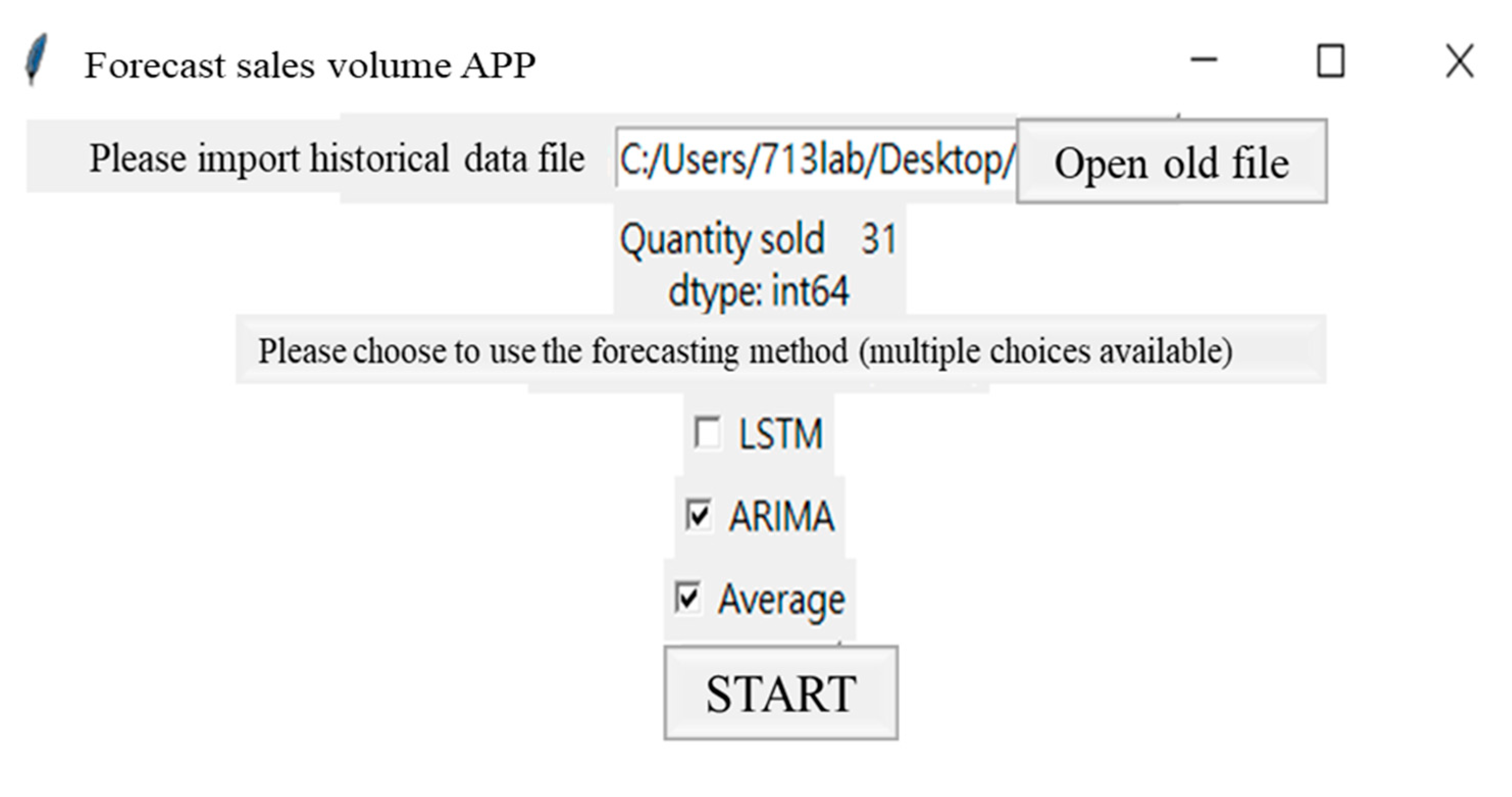
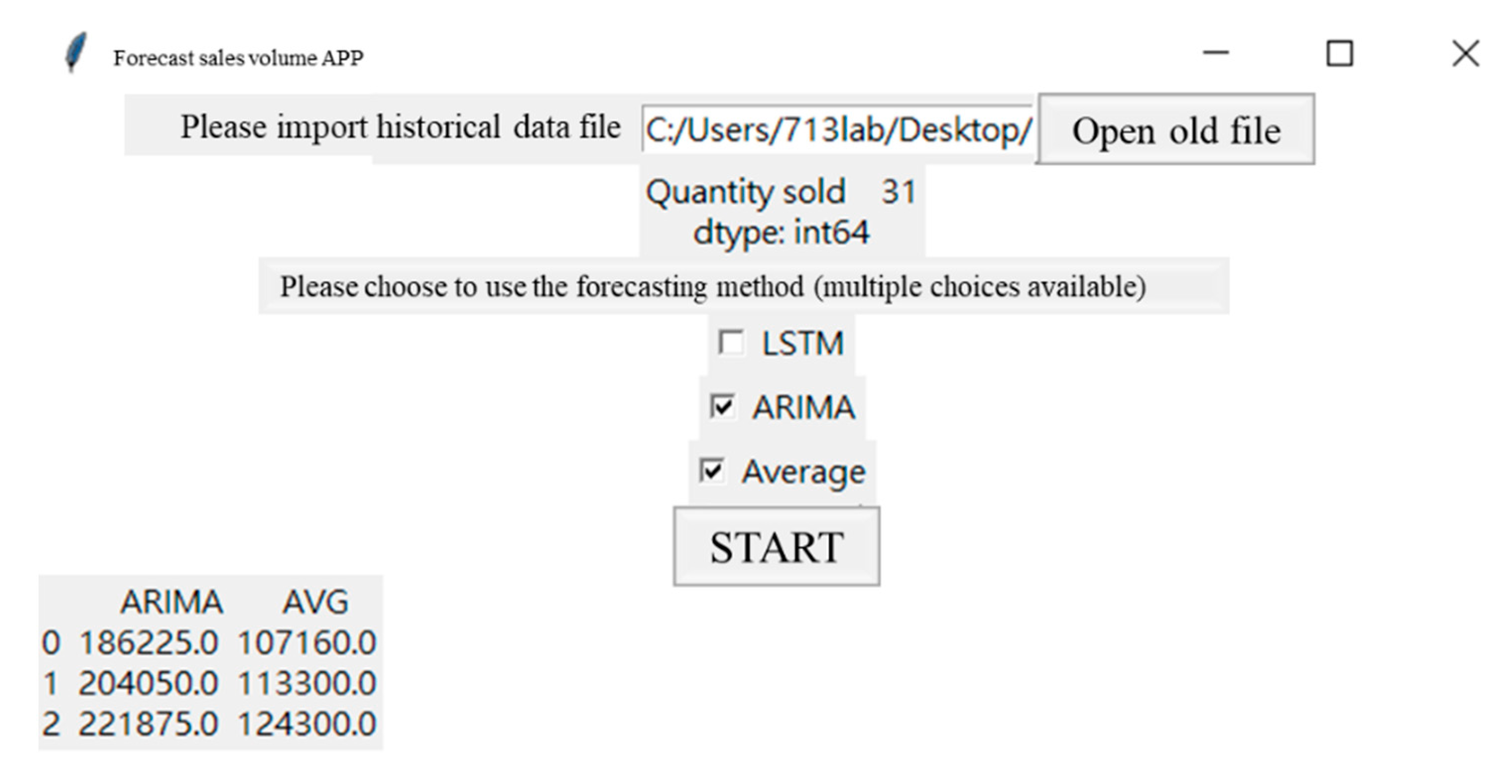
The following describes the time-series analysis for the recent discussion where many scholars are committed to this part of the study. The top five products accounted for a considerable proportion of the case companies for the prediction model object, the application of the actual information within the case company, the prediction model based on statistical time-series methods, and neural methods for the following research conclusions and follow-up research recommendations.

ARIMA and LSTM are two predictive models that predict the top five products and validate the actual data and prediction results with RMSE to evaluate the prediction model’s performance. As a result, LSTM has the smallest forecast error in the short-term forecast. Thus, the superior quantity-forecasting model for the demand market is the fast and accurate short-term forecast model. This forecast model could provide managers as a reference for procurement. There are superior and inferior models, and the ARIMA advantage model is very simple, requiring only endo-variables without the need for other exo-variables. Cons: First, the time-series data must be stable (stationary) or stable after differentiation (differential). Second, only linear relationships can be captured in essence, not nonlinear relationships. The advantages of LSTM complement the ARIMA disadvantages, which do not require sequence stabilization before modeling. Conversely, the disadvantage of LSTM is that the parameter setting is complex.

Validated by actual data and prediction results, it is confirmed that the prediction model proposed in this study has a better prediction model. This study provides a tkinter package that creates a GUI library in python that can be intuitively embedded into an enterprise system. Whenever the data are updated, it is only necessary to put in the files of sales time and sales quantity of various products to predict the sales quantity in different ways, and for the next three weeks, in about 10 s. This research uses Plato’s 80/20 rule is to obtain the company’s top five products to make predictions. However, the few key products vary over time. Therefore, it is necessary to import a new Excel file to update the data to make the prediction results more referenced. The company’s empirical rule (MA = 5), the exponential smoothing method in the traditional time-series method, and the ARIMA and LSTM prediction model used in this research in forecasting the sales volume are averaged with the above four methods. Automatic forecasting model: the maximum number of forecast periods in the system is 3 in this study, to improve forecasting accuracy. The weekly or monthly forecasted sales quantity for a specific product can facilitate the case company with future orders and the reference basis for inventory management. The following are the process steps of the forecast demand system:

Step 1:

select the forecast item number.

As in Figure 7, please click to open the old file in the frame of importing the historical data file. Click to open the old file and search for the position of the part number you want to predict (such as part number QFN9X9).

Step 2:

select prediction method.

As in Figure 8, the location of the item number database is displayed in the frame of “Please import the historical data file”; the number of historical data for quantity sold is displayed below, and you can select the forecasting method you want to use (multiple selections).

Step 3:

forecast sales quantity.

As in Figure 9, after selecting the forecast method, the sales quantity of the selected forecast method is directly displayed below.

After the actual data and forecast results are verified, it is confirmed that the forecast model proposed by this research institute has a better predictive ability table, and some suggestions are put forward here for the follow-up researchers for reference. (1) Add key influencer factors. Many factors influence the change of product order demand. Over time, the selection of crucial influence factors changes. Therefore, we try to find more key influence factors that may affect product price changes through the data exploration method. We increase the influence factors with high correlation to improve the predictive ability of the forecast model. (2) More comparisons of the predictive model. In this study, ARIMA and LSTM are constructed with statistical time series and neural network methodology and compared according to the prediction results, and now there are many artificial intelligence prediction methods. The follow-up researchers can establish more different prediction models, such as gene algorithm, bee swarm algorithm, and particle group algorithm. By comparing more forecasting models, the best forecasting models are selected to construct product demand forecasting models.

References

1. Wu, H.Y.; Chen, I.S.; Chen, J.K.; Chien, C.F. The R&D efficiency of the Taiwanese semiconductor industry. Measurement 2019, 137, 203–213. [Google Scholar]
2. International Data Corporation. Worldwide Semiconductor Revenue Grew 5.4% in 2020 Despite COVID-19 and Further Growth Is Forecast in 2021, According to IDC. Available online: https://www.idc.com/getdoc.jsp?containerId=prUS47424221 (accessed on 11 February 2021).
3. Taiwan Semiconductor Industry Association. TSIA Q4 2020 and Year 2020 Statistics on Taiwan IC Industry. TSIA Report. Available online: https://www.tsia.org.tw/PageContent?pageID=1 (accessed on 20 February 2021).
4. Nian, S.C.; Fang, Y.C.; Huang, M.S. In-mold and machine sensing and feature extraction for optimized IC-tray manufacturing. Polymers 2019, 11, 1348. [Google Scholar] [CrossRef] [PubMed] [Green Version]
5. Karimnezhad, A.; Moradi, F. Bayes, E-Bayes and robust Bayes prediction of a future observation under precautionary prediction loss functions with applications. Appl. Math. Model. 2016, 40, 7051–7061. [Google Scholar] [CrossRef]
6. Moon, M.A. Demand and Supply Integration: The Key to World-Class Demand Forecasting; Walter de Gruyter GmbH & Co KG: Berlin, Germany, 2018. [Google Scholar]
7. Bruzda, J. Demand forecasting under fill rate constraints—The case of re-order points. Int. J. Forecast. 2020, 36, 1342–1361. [Google Scholar] [CrossRef]
8. Abadi, S.N.R.; Kouhikamali, R. CFD-aided mathematical modeling of thermal vapor compressors in multiple effects distillation units. Appl. Math. Model. 2016, 40, 6850–6868. [Google Scholar] [CrossRef]
9. Nia, A.R.; Awasthi, A.; Bhuiyan, N. Industry 4.0 and demand forecasting of the energy supply chain: A. Comput. Ind. Eng. 2021, 154, 107128. [Google Scholar]
10. Hu, M.; Qiu, R.T.; Wu, D.C.; Song, H. Hierarchical pattern recognition for tourism demand forecasting. Tour. Manag. 2021, 84, 104263. [Google Scholar] [CrossRef]
11. Kozik, P.; Sp, J. Aircraft engine overhaul demand forecasting using ANN. Manag. Prod. Eng. Rev. 2012, 3, 21–26. [Google Scholar]
12. Gutierrez, R.S.; Solis, A.O.; Mukhopadhyay, S. Lumpy demand forecasting using neural networks. Int. J. Prod. Econ. 2008, 111, 409–420. [Google Scholar] [CrossRef]
13. Willemain, T.R.; Smart, C.N.; Schwarz, H.F. A new approach to forecasting intermittent demand for service parts inventories. Int. J. Forecast. 2004, 20, 375–387. [Google Scholar] [CrossRef]
14. Dunn, W.N. Poblicy Analysis: An Introduction, 2nd ed.; Prentice Hall Englewood Cliffs: Hoboken, NJ, USA, 1994. [Google Scholar]
15. Rosienkiewicz, M.; Chlebus, E.; Detyna, J. A hybrid spares demand forecasting method dedicated to mining industry. Appl. Math. Model. 2017, 49, 87–107. [Google Scholar] [CrossRef]
16. Box, G.E.P.; Jenkins, G.M. Time Series Analysis: Forecasting and Control; Holden-Day: San Francisco, CA, USA, 1976. [Google Scholar]
17. Siami-Namini, S.; Tavakoli, N.; Namin, A.S. A comparison of ARIMA and LSTM in forecasting time series. In Proceedings of the 2018 17th IEEE International Conference on Machine Learning and Applications (ICMLA), Orlando, FL, USA, 17–20 December 2018; pp. 1394–1401. [Google Scholar]
18. Fattah, J.; Ezzine, L.; Aman, Z.; El Moussami, H.; Lachhab, A. Forecasting of demand using ARIMA model. Int. J. Eng. Bus. Manag. 2018, 10, 1847979018808673. [Google Scholar] [CrossRef] [Green Version]
19. Salman, A.G.; Kanigoro, B. Visibility forecasting using autoregressive integrated moving average (ARIMA) models. Procedia Comput. Sci. 2021, 179, 252–259. [Google Scholar] [CrossRef]
20. Roondiwala, M.; Patel, H.; Varma, S. Predicting stock prices using LSTM. Int. J. Sci. Res. 2017, 6, 1754–1756. [Google Scholar]
21. Pacella, M.; Papadia, G. Evaluation of deep learning with long short-term memory networks for time series forecasting in supply chain management. Procedia CIRP 2021, 99, 604–609. [Google Scholar] [CrossRef]
22. Pak, U.; Ma, J.; Ryu, U.; Ryom, K.; Juhyok, U.; Pak, K.; Pak, C. Deep learning-based PM2.5 prediction considering the spatiotemporal correlations: A case study of Beijing, China. Sci. Total Environ. 2020, 699, 133561. [Google Scholar] [CrossRef]
23. Chien, C.F.; Hong, T.Y.; Guo, H.Z. An empirical study for smart production for TFT-LCD to empower Industry 3.5. J. Chin. Inst. Eng. 2017, 40, 552–561. [Google Scholar] [CrossRef]
24. Dickey, D.A.; Fuller, W.A. Distribution of the estimators for autoregressive time series with a unit root. J. Am. Stat. Assoc. 1979, 74, 427–431. [Google Scholar]
25. Kwiatkowski, D.; Phillips, P.C.; Schmidt, P.; Shin, Y. Testing the null hypothesis of stationarity against the alternative of a unit root: How sure are we that economic time series have a unit root? J. Econom. 1992, 54, 159–178. [Google Scholar] [CrossRef]
26. Said, S.E.; Dickey, D.A. Testing for unit roots in autoregressive-moving average models of unknown order. Biometrika 1984, 71, 599–607. [Google Scholar] [CrossRef]
27. Abbasimehr, H.; Shabani, M.; Yousefi, M. An optimized model using LSTM network for demand forecasting. Comput. Ind. Eng. 2020, 143, 106435. [Google Scholar] [CrossRef]
28. Priya, C.B.; Arulanand, N. Univariate and multivariate models for Short-term wind speed forecasting. Mater. Today Proc. 2021. [Google Scholar] [CrossRef]
29. Shi, H.; Xu, M.; Li, R. Deep learning for household load forecasting—A novel pooling deep RNN. IEEE Trans. Smart Grid 2017, 9, 5271–5280. [Google Scholar] [CrossRef]
30. Kong, W.; Dong, Z.Y.; Jia, Y.; Hill, D.J.; Xu, Y.; Zhang, Y. Short-term residential load forecasting based on LSTM recurrent neural network. IEEE Trans. Smart Grid 2017, 10, 841–851. [Google Scholar] [CrossRef]
31. Lewis, C.D. International and Business Forecasting Methods; Butterworths: London, UK, 1982. [Google Scholar]
32. Weng, B.; Martinez, W.; Tsai, Y.T.; Li, C.; Lu, L.; Barth, J.R.; Megahed, F.M. Macroeconomic indicators alone can predict the monthly closing price of major US indices: Insights from artificial intelligence, time-series analysis and hybrid models. Appl. Soft Comput. 2018, 71, 685–697. [Google Scholar] [CrossRef]
33. Qiao, W.; Wang, Y.; Zhang, J.; Tian, W.; Tian, Y.; Yang, Q. An innovative coupled model in view of wavelet transform for predicting short-term PM10 concentration. J. Environ. Manag. 2021, 289, 112438. [Google Scholar] [CrossRef]
Figure 1. Prediction method hierarchy diagram.
Processes 09 01157 g001
Figure 2. Research framework flow chart.
Processes 09 01157 g002
Figure 4. Average square root error assessment graph for empty value processing. (a) Retaining the original data; (b) deleting the null value; (c) replacing the null value with the high-frequency technique; (d) replacing the null value with the average value.
Processes 09 01157 g004
Figure 5. Rolling forecast schematic.
Processes 09 01157 g005
Figure 6. A diagram of a rolling forecast. (a) Predicted five values in the test set; (b) predicted the second to fifth data of the test set; (c) predicted the third to fifth strokes of the test set.; (d) predicted the fourth to fifth data of the test set; (e) predicted of the fifth demand in the test set.
Processes 09 01157 g006
Figure 7. Select the forecast item number.
Processes 09 01157 g007
Figure 8. Method filters the schematic.
Processes 09 01157 g008
Figure 9. The number of periods filtered indicates.
Processes 09 01157 g009