Numerical Analysis and Optimization of Solar-Assited Heat Pump Drying System with Waste Heat Recovery Based on TRNSYS

Abstract

In this paper, a new solar-assisted heat pump drying system with waste heat recovery and double water tanks (SCAHP) was established and the system optimized by TRNSYS and variable air volume experiment. The annual cumulative efficiency of the SCAHP (COP_ac), buffer tank heating efficiency (η_BT) and hot water storage tank heating efficiency (η_ST) are all considered as optimization objectives, and this paper discusses the relationship between the three optimization objectives and studies the influence of hot air volume (q_DR), area of solar collector (A_SC), inclination angle of solar collector (I_SC) and volume of heat storage water tank (V_ST) on system efficiency in the drying process. In order to explore the general rule of system optimization, numerical analysis and optimization were carried out in five typical cities in five climatic regions of China. The results show that the mixed variable air volume mode can increase the drying rate with less energy loss, and shorten the drying period by 28.6–33.3%. When the system surface body ratio (SBR) in Nanjing is between 3.1 and 4.1, the COP_ac, η_BT, and η_ST can reach the maximum value simultaneously. It is estimated that the cost can be recovered in 5 years when the system configuration parameters are optimized.

1. Introduction

Drying has a large number of applications in industry, agriculture and other fields, while drying is one of the most energy-consuming units [1]. In developed countries, about 10% of fuel is used for drying, and in China, drying energy consumption accounts for about 12% of the entire industrial energy consumption [2]. In some industries, the energy waste caused by drying is enormous, with Mujumdar [3] reporting that drying consumes up to 70% of the total energy in the manufacture of wood products, 50% of the total energy in the manufacture of finished textiles, and over 60% of the total energy in agricultural maize production. In order to develop sustainable energy sources, three important technological changes are required: energy conservation on the demand side, increased efficiency in energy production, and the replacement of fossil fuels with various renewable sources [4]. In this regard, the use of heat pump drying systems and solar heat collecting systems has improved energy efficiency and reduced consumption of fossil fuels.

The energy efficiency of traditional dryers is usually very low. Lawton J [5] points out that the efficiency of traditional dryers can only reach 35% at the highest. Queiroz R [6] found that heat pump drying saves 40% energy in comparison with using electrical heater dryers. The traditional dryer is not only inefficient, but also the quality of drying products is not up to the requirements. With the rapid development of industry and agriculture, vacuum drying, freeze drying, spray drying and other methods have been put forward one after another; however, these drying processes are highly energy-intensive and have the disadvantages of high economic costs or low drying rates, and the advantages of heat pump drying are further prominent. In some studies, heat pump drying is considered to provide better product quality under the premise of lower energy consumption [7,8,9,10,11]. The first batch of heat pump drying studies in the literature was completed by Hodgett [12] and Geeraert [13]. In recent decades, many scientists have studied how to improve the efficiency of heat pump systems from various aspects [14,15,16]. However, related studies show that heat pump technology still has problems such as using high-grade electric energy, the small drying scale of single heat pumps and high system maintenance costs [17,18].

The combination of multiple energy sources, especially the introduction of renewable energy, has become one of the current research hotspots. Solar energy has attracted much attention as the most readily available renewable energy source. Open solar drying is the earliest drying technology that has been applied [19], but its external drying conditions are difficult to be controlled, resulting in too-long drying times of materials or poor quality of dried products. The efficiency of solar direct drying of crops is between 20–40% [20]. To solve these problems, many scientists are trying to combine solar drying with heat pump technology.

Luo Huilong et al. [21] designed and constructed an air source heat pump-assisted solar energy drying system. Compared with conventional drying systems, the air source heat pump-assisted solar energy drying system has greater energy saving potential. Rahman et al. [22] economically optimized the evaporator and air collector of a solar-assisted heat pump drying system. Their economic analysis showed that using an air collector area of 1.25 m² and an evaporator collector area of 2 m², the system had significant cost savings with a payback period of 4.4 years. In a recent work, Meltem [23] et al. designed and tested a new type of sustainable photovoltaic/heat-assisted heat pump drying. The results show that the average coefficient of performance of the heat pump can reach 4.18, according to solar radiation and ambient temperature, and an average electric efficiency of 12.27% and a maximum of 14.02% can be obtained.

However, in the drying system combined with solar energy and heat pump, there is often a mismatch between energy supply and demand and excessive waste heat waste. Energy storage technology can solve this problem well. The application of heat storage in the solar drying system is justified under the following three circumstances [24]: (1) the drying period can be prolonged by energy storage; (2) the excess energy at the peak of radiation can be stored to avoid excessive local drying; and (3) the temperature of dry air can be controlled to avoid damage to materials. Qiu et al. [25] used a solar-assisted heat pump drying system with heat recovery to dry 10 kg of carrots, and the results showed that the system saved about 40.5% of the energy. Wang et al. [26] studied the use of another form of solar-assisted heat pump drying system with heat recovery to dry 80 kg of mangoes, and the results showed that the efficiency of the system was improved by about 6%, and the waste heat recovery rate reached 41.7%.

On the basis of predecessors’ research, this paper proposes a new solar-assisted heat pump drying system with waste heat recovery and double water tanks, where the waste heat recovery module can partially offset the variable air volume of energy loss. On the basis of experiment explores the influence of variable air volume on the drying process, and system efficiency, the whole-year numerical simulation is carried out based on TRNSYS, and the parameters and operation parameters of each component of the system are optimized.

2. System Model and Research Method

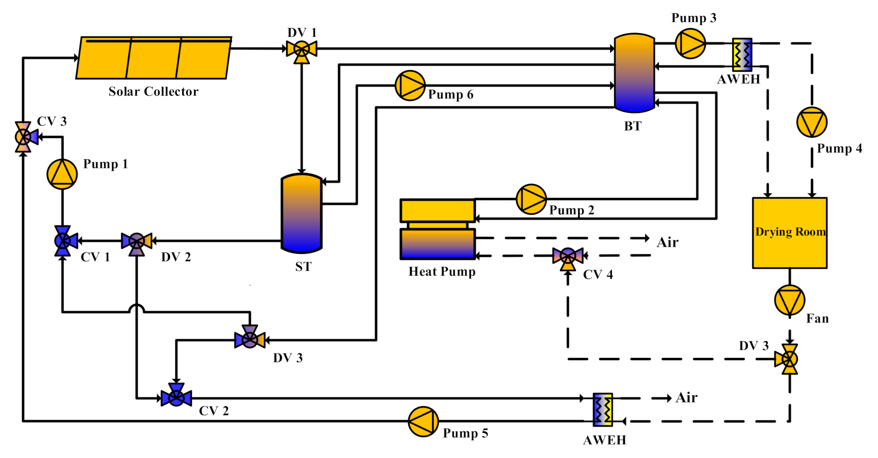
2.1. Introduction of SCAHP

Figure 1 shows the schematic diagram of SCAHP. The system includes a solar collector (SC), air-water heat exchanger (AWEH), buffer tank (BT), hot water storage tank (ST), air-water heat pump (HP), water pump, fan and drying room (DR). The parameters of system components, operation parameters and corresponding variation ranges are shown in

Table 1. Characteristics of the instruments.

Name	Reference Value	Range
ISC	30°	15°~50°
ASC	0.3 m2	0.1 m2~0.8 m2
SC Efficiency	Optional efficency: 0.8, heat loss coefficient: 0.78 W/(m2·°C)	–
VBT	0.05 m3	–
VST	0.04 m3	0.2 m3~0.4 m3
HP	Output = 1.5 kW	–
Pump 1 flow	21 kg/h	–
Pump 3 flow	250 kg/h	–

. Among them, the fan is a forced convection fan installed at the outlet of DR, so as to facilitate the variable air volume drying experiment and waste heat recovery.

All energy consumption of DR is provided by BT, the heat of BT comes from SC, HP, ST and waste heat recovery, the heat of ST comes from the SC and waste heat recovery, and the heat recovered from waste heat can be used in two ways: first, passing the waste hot air directly to the low temperature side of the HP through the fan; second, passing the waste hot air to the SC inlet side after being converted by AWEH.

The SC and HP are connected in parallel, and the start and stop of the SC circuit is not directly related to the start and stop of the HP circuit. When the temperature of the BT is insufficient, the SC is first opened for heating, that is, pump 1 is turned on, and priority is given to the heat supply to the BT. The above can be expressed as that the hot water in the SC flows to the BT through DV 1, and then flows back to the SC through DV 3, CV 1, Pump 1, and CV 3 after coming out of the BT. When the temperature of the BT reaches the set value, but the temperature of the ST does not reach the set value, the hot water in the SC flows to the ST through DV 1, and passes through DV 2, CV 1, Pump 1 and CV 3 after coming out of the ST flow back to the SC. When the temperature of the BT and ST reach the set value, the SC circuit is closed. When the temperature in the BT is lower than a set value lower than the set temperature of the SC circuit, the HP and Pump 2 are turned on, and the hot water flows into the BT and returns to the HP until the BT reaches the set upper limit and closes the loop.

Waste heat recovery can be achieved by passing the waste heat to the inlet of the SC or the low temperature side of the HP through the fan. There are two points to note: 1, the carrier of waste heat recovery heat is air. When it leads to the low temperature side of the SC, it needs to be converted by a water-air heat exchanger. At the inlet of the SC, it is mixed with the return water of the original SC circuit, heated by the SC, and then led to the BT or ST. 2, When the heat recovered by the waste heat directly passes to the low temperature side of the HP, it may not be able to meet the flow demand of the low temperature side of the HP. At this time, the hot air from the waste heat recovery needs to be mixed with the air in the atmospheric environment, that is, pass through CV 4 to the low temperature side of the HP.

The heat supply from the ST to the BT is only related to the temperature difference between the two water tanks, and whether the BT reaches the set temperature is related. From the perspective of heat supply, the heat supply from the ST is in parallel with the heat supplied by the SC and HP. When the heating conditions are met, pump 6 is turned on, and the hot water flows from the ST to the BT and returns to the ST. It should be noted that the control logic of this system and the set temperature range of each loop will be described in detail in Section 2.2 Control Logic.

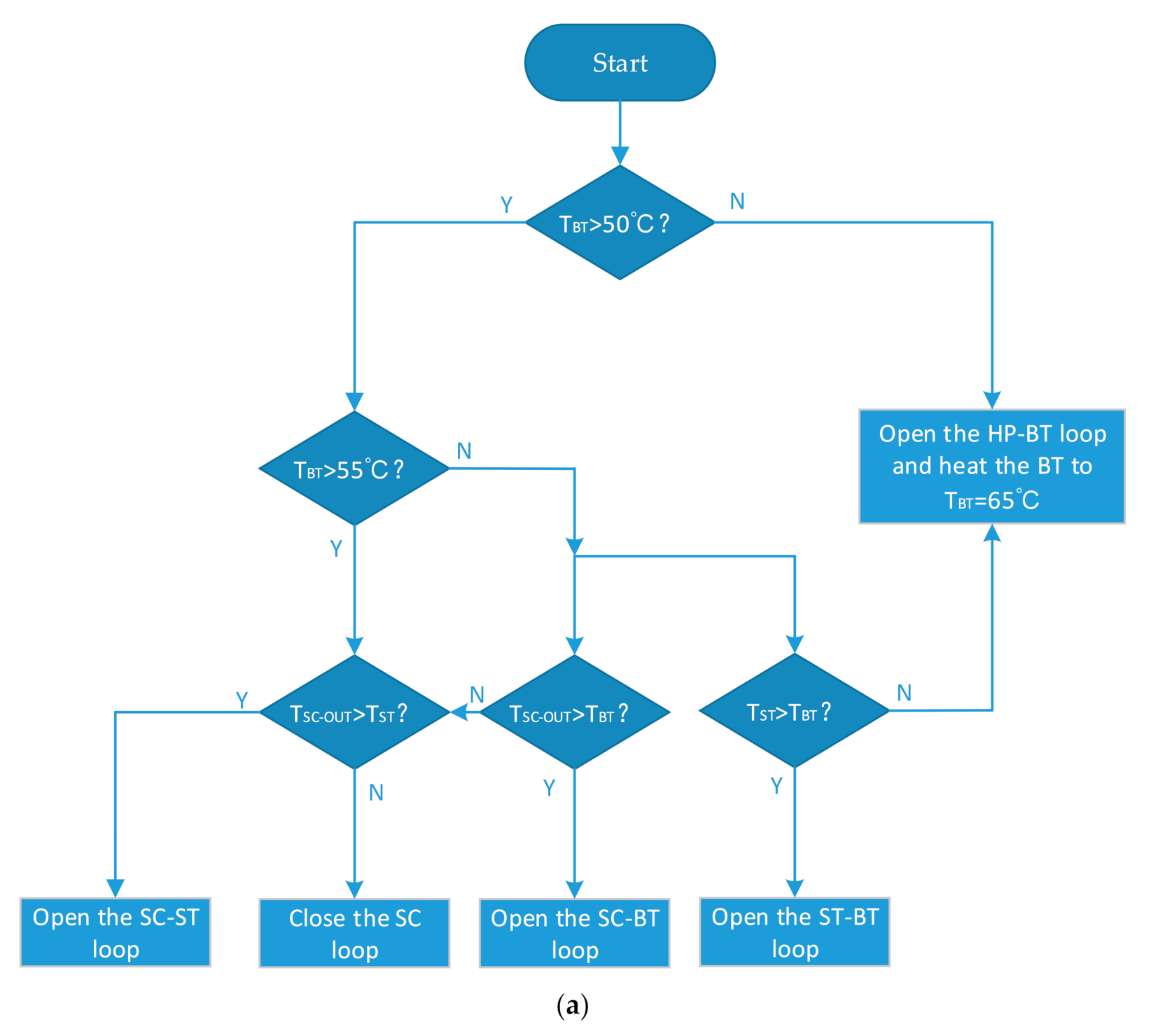
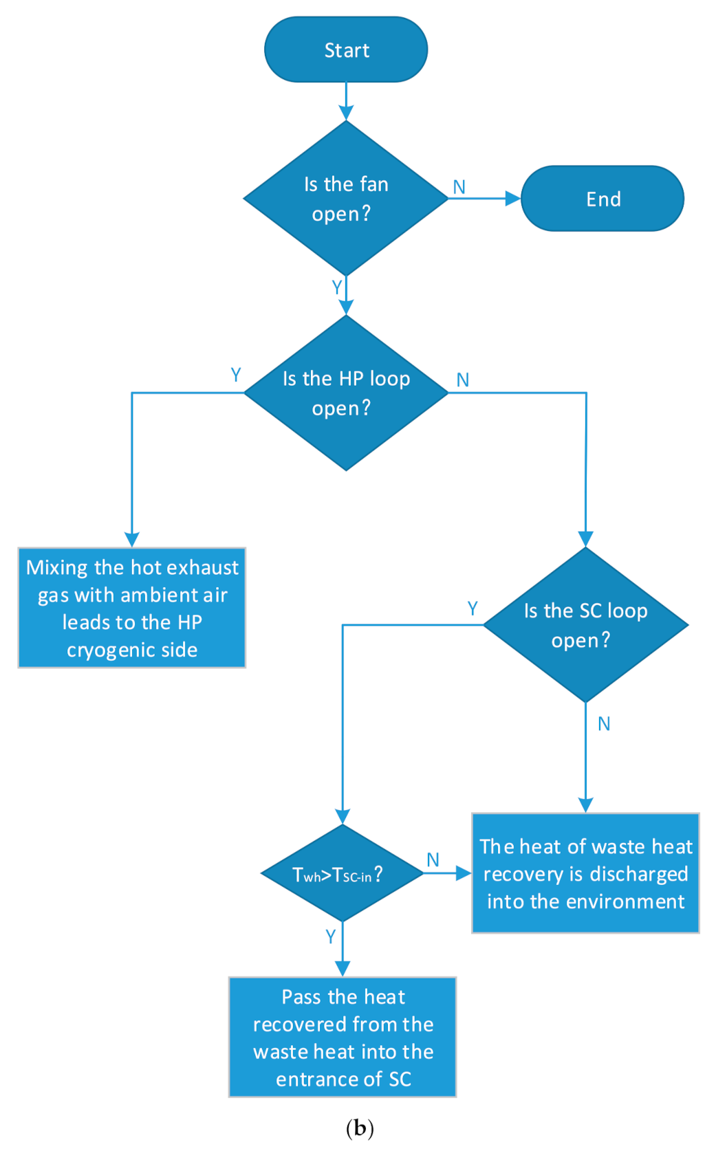
2.2. Control Logic of SCAHP

Figure 2a,b are combined to show the complete control logic of SCAHP. Figure 2a shows the control logic of SCAHP except for the waste heat recovery module. The figure also provides the temperature settings of the water tank in each heating mode mentioned in Section 2.1. According to the temperature value of the BT, the control mode of the system is divided into three modes.

Mode 1: If the average temperature of BT (T_BT) is lower than 50 °C, turn on the HP to heat the BT to 65 °C, and then turn off the HP. At the same time, it is judged whether the outlet temperature of SC (T_SC-OUT) or the outlet temperature of ST (T_ST) is greater than T_BT. When the judgment value is 1, the heating circuit of the SC or ST is started to heat the BT to 55 °C. When T_BT reaches 55 °C or T_SC-OUT is less than T_BT, judge whether T_SC-OUT is greater than T_ST. When the judgment value is 1, the SC transfers heat to the ST.

Mode 2: When T_BT is greater than 50 °C and less than 55 °C, it is judged whether T_SC-OUT or T_ST is greater than T_BT. When the judgment value is 1, the SC or ST is activated to transfer heat to the BT until T_BT gets to 55 °C, When T_BT reaches 55 °C or T_SC-OUT is less than T_BT, judge whether T_SC-OUT is greater than T_ST. When the judgment value is 1, the SC is started to transfer heat to the ST, otherwise SCAHP is in shutdown state, and T_BT gradually drops and enters mode 1.

Mode 3: When the temperature of the BT is greater than 55 °C, it is judged whether the outlet temperature of the SC is greater than the temperature of the ST. When the judgment value is 1, the SC will be started for heating, otherwise the system is in shutdown state, and the temperature of the BT will gradually drop into mode 2.

Figure 2b shows the control logic of the system’s waste heat recovery module. The first thing to note is that when the waste heat recovery fan is not turned on, the waste heat mode is turned off and the system does not enter this control module. When the fan is turned on, first determine whether the HP is turned on. When the HP is turned on, the hot air obtained in the waste heat recovery and ambient air will be mixed and sent to the low temperature side of the HP. If the HP is in a shutdown state, judge whether the SC circuit is open, and whether the temperature of the hot water exchanged with the hot air recovered by the waste heat in the heat exchanger is greater than the inlet temperature of the SC; when the two judgments both return the value 1, the heat recovered by the waste heat is led to the entrance of the SC, otherwise the waste heat is directly discharged into the surrounding environment.

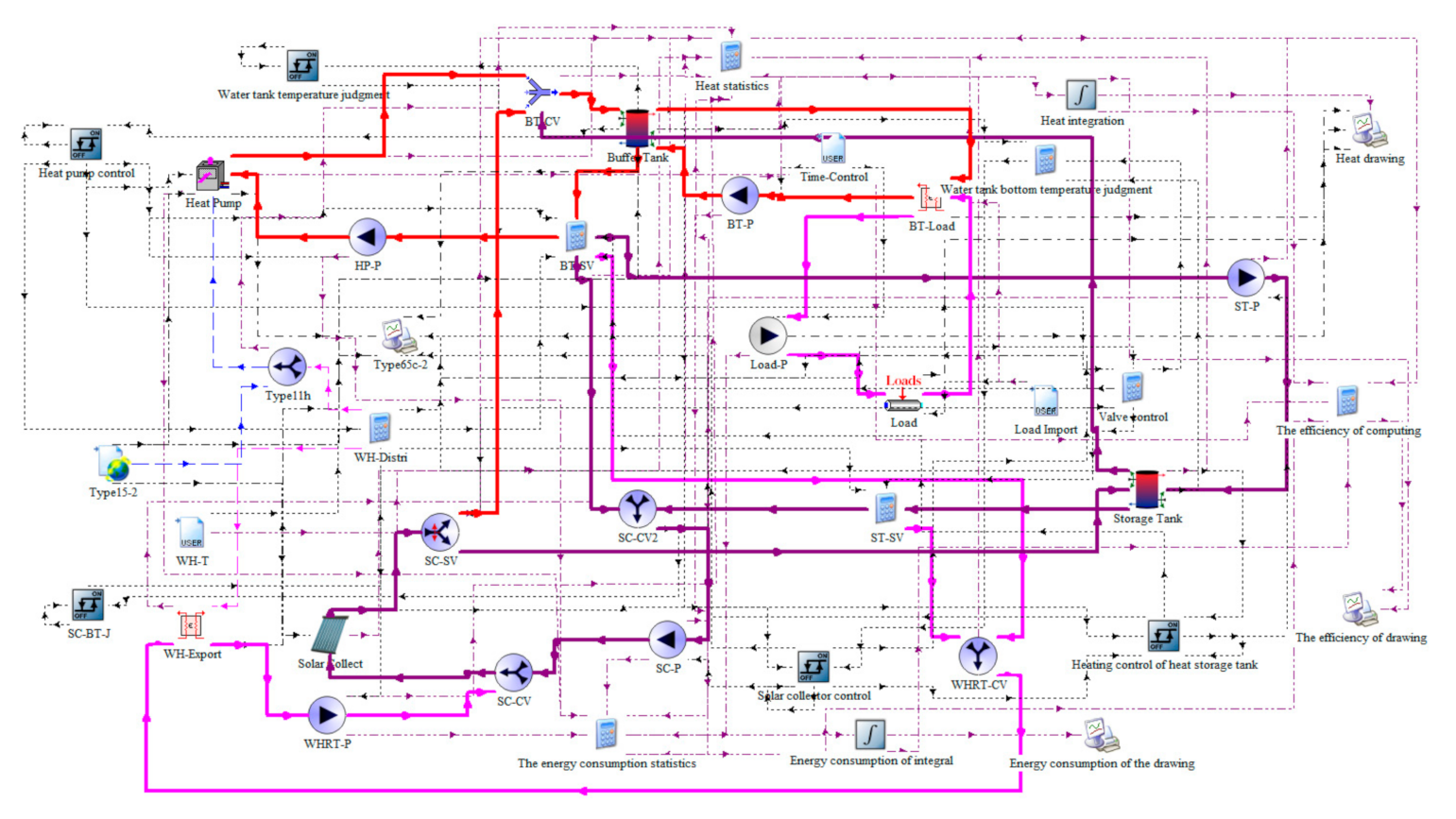
2.3. TRNSYS Simulation Model of SCAHP

According to the SCAHP physical model, control logic and parameter settings described above, a system simulation model is established in TRNSYS 17. TRNSYS (Transient System Simulation Program) is an extremely flexible graphically based software environment used to simulate the behavior of transient systems, and most TRNSYS-based simulations focus on evaluating the performance of thermal and electrical energy systems. The model contains weather file, SC, HP, BT, ST, DR, water pump, fan, heat exchanger and control strategy. The main components of the TRNSYS simulation model and their descriptions are shown in

Table 2. Main component in TRNSYS.

Name	Component Type	Descriptions
Weather data	$\mathrm{Type} 152$	This component serves the purpose of reading data at regular time intervals from an external weather data file
Tank	$\mathrm{Type} 4$	Thermal storage device
Heat pump	$\mathrm{Type} 941$	This component models a single-stage air to water heat pump
pump	$\mathrm{Type} 114$	Type114 models a single (constant) speed pump that is able to maintain a constant fluid outlet mass flow rate
Flow diverter	$\mathrm{Type} 649/11\mathrm{f}$	Two inlet liquid flows are mixed into a single liquid outlet flow
Flow mixer	$\mathrm{Type} 11\mathrm{h}$	A single inlet liquid outlet flow is divided into two outlet liquids
Temperature judgement	$\mathrm{Type} 2\mathrm{b}$	The on/off differential controller generates a control function which can have a value of 1 or 0.
Drying room	$\mathrm{Type} 682$	This model simply imposes a user-specified load (cooling = positive load, heating = negative load) on a flow stream and calculates the resultant outlet fluid conditions.

.

When performing model verification, the time step is set to 1 min, which is controlled at the same magnitude as the time step of the verification object. In the simulation analysis of the whole year, the step length is set to 1 h. The system control strategy is implemented by Type 2b and calculator. The shunt valve at the outlet of the BT and ST is replaced by a calculator. The TRNSYS simulation model diagram is shown in Figure 3.

2.4. Research Method

This research adopts a combination of experiment and simulation, taking 731 g of carrots as the experimental material, and exploring the influence of variable air volume on material drying, suitable variable air volume control modes, drying rate and energy consumption data of different variable air volume modes in the variable air volume experiment. Exploring the optimal configuration and optimal operating parameters of the system in the simulation, input of the real-time data of the DR energy consumption is obtained through the experiment through Type 682. Taking COP_ac, η_BT and η_ST as optimization goals, orthogonal experiments are used to optimize A_SC, I_SC and V_ST. Finally, the economic performance of the system is also verified.

This study takes five typical cities in China’s five major climate regions as the research objects, namely Harbin, Tianjin, Nanjing, Guangzhou, and Kunming, to explore the general laws of the system proposed in this paper. In the simulation calculation, the meteorological parameters are based on the typical yearly parameters of five cities. The typical meteorological year (TMY) is based on the monthly average of the past 10 years. The parameters of the five cities are shown in

Table 3. Basic Parameters of Typical Cities in Five Climate Zones of China.

Name	Climate Region	$\mathbf{Longitude} (°)$	$\mathbf{Latitude} (°)$	$\mathbf{Average} \mathbf{Temperature} \mathbf{of} \mathbf{the} \mathbf{Coldest} \mathbf{Month} \left(°\mathbf{C}\right)$	$\mathbf{Average} \mathbf{Temperature} \mathbf{of} \mathbf{the} \mathbf{Hottest} \mathbf{Month} (°\mathbf{C})$
Harbin	Severe cold area	126.77	45.75	−16.9	23.8
Tianjin	Cold area	117.17	39.93	−2.9	27.1
Nanjing	Hot summer and cold winter area	118.80	32.00	3.1	28.3
Guangzhou	Hot summer and warm winter area	113.33	23.17	14.3	28.8
Kunming	Temperate area	102.65	25.00	9.4	20.3

. Taking Nanjing City as the main analysis object, the analysis and optimization results of other cities will be summarized in the table and given uniformly. It should be pointed out that in our model only the difference in ambient temperature and solar radiation between different cities is considered.

3. Mathematical Model

3.1. Total Heat Required for Drying Process

The heat consumed by carrots during the drying process can be divided into three parts: The heat required for preheating carrots, the heat required for evaporation of water from carrots, and the heat loss of the entire system during the drying process. According to the first law of thermodynamics:

$$Q_t=Q_p+Q_e+Q_l$$

(1)

The heat required for the carrot preheating stage is:

$$Q_p=c_r{m}_{r0}\left(T_{r1}-T_{r0}\right)$$

(2)

where $c_r$ is the specific heat of the carrot under constant pressure $\left(\mathrm{kJ}/\mathrm{kg}·\mathrm{k}\right)$, $m_{r0}$ is the initial mass of the carrot $\left(\mathrm{kg}\right)$, and $T_{r0}$ is the carrot temperature before preheating $\left(°\mathrm{C}\right)$, equivalent to ambient temperature, and $T_{r1}$ is the carrot temperature after preheating $\left(°\mathrm{C}\right)$, equivalent to the temperature after the constant temperature of the DR stabilizes.

The heat required by carrots to evaporate water is:

$$Q_e=\gamma ·\left(m_{r0}-m_{r2}\right)$$

(3)

where $\gamma$ is the latent heat of vaporization of the moisture in the carrot $\left(\mathrm{kJ}/\mathrm{kg}\right)$, and $m_{r2}$ is the mass of the carrot after the drying $\left(\mathrm{kg}\right)$.

The heat loss during the drying process of carrot is:

$$Q_l=\left(Q_p+Q_e\right)\times 10\%$$

(4)

3.2. Solar Collector

The total amount of radiation during the working hours of SC is:

$$G=3.6{{\displaystyle \int }}_0^{t_1}{A}_c{I}_{t}dt$$

(5)

where $A_c$ is the area of the solar collector $\left({\mathrm{m}}^2\right)$, $I_t$ is the instantaneous solar radiation value incident on the SC, W/m², and $t_1$ is the total open time of the SC $\left(\mathrm{h}\right)$.

The energy used by the SC to provide the DR is:

$$Q_{sc}={\eta }_{BT}{\eta }_{AWHE}\left[G·{\eta }_{sc}+\left({\eta }_{ST}-1\right)\times Q_{SC-ST}\right]$$

(6)

where $G$ is the total energy received by the SC $\left(\mathrm{kJ}\right)$, ${\eta }_{sc}$ is the conversion efficiency of SC, ${\eta }_{BT}$ is the heating efficiency of the BT, ${\eta }_{ST}$ is the heating efficiency of the ST, ${\eta }_{AWHE}$ is the heat exchange efficiency of the air-water heat exchanger, the air-water heat exchange efficiency of the system is set to a fixed value, 0.65, and $Q_{SC-ST}$ is the total energy obtained by the ST from the SC $\left(\mathrm{kJ}\right)$.

The total heating share (SF) of the system occupied by the heat supply of solar collectors can be expressed as:

$$SF=Q_{sc}/Q_t$$

(7)

3.3. Tank

The heat supplied by the SC to the BT is:

$$Q_{SC-BT}=3600{{\displaystyle \int }}_0^{t_2}{m}_{sc}{c}_{sc}\left(T_{scout}-T_{scin}\right)dt$$

(8)

The heat supplied by the SC to the ST is:

$$Q_{SC-ST}=3600{{\displaystyle \int }}_0^{t_3}{m}_{sc}{c}_{sc}\left(T_{scout}-T_{scin}\right)dt$$

(9)

where $m_{sc}$ is the mass flow of water passing through the solar collector $\left(\mathrm{kg}/\mathrm{s}\right)$, $c_{sc}$ is the specific heat of water under constant pressure kJ/kg·k, and $T_{scout}$ is the outlet temperature of the SC $\left(°\mathrm{C}\right)$, $T_{scin}$ is the inlet temperature of the SC $\left(°\mathrm{C}\right)$, $t_2$ is the time it takes for SC to supply heat to the BT $\left(\mathrm{h}\right)$,$t_3$ is the time it takes for the SC to supply heat to the ST $\left(\mathrm{h}\right)$.

The heat supplied by the HP to the BT is:

$$Q_{HP-BT}=3600{{\displaystyle \int }}_0^{t_4}{m}_{HP}{c}_{HP}\left(T_{HPout}-T_{HPin}\right)dt$$

(10)

where $m_{HP}$ is the mass flow of water passing through HP $\left(\mathrm{kg}/\mathrm{s}\right)$, $c_{HP}$ is the specific heat of water under constant pressure $\left(\mathrm{kJ}/\mathrm{kg}·\mathrm{k}\right)$, and $T_{HPout}$ is the outlet temperature on the condenser side of the HP $\left(°\mathrm{C}\right)$, $T_{HPin}$ is the inlet temperature on the condenser side of the HP $\left(°\mathrm{C}\right)$, $t_4$ is the total open time of the HP $\left(\mathrm{h}\right)$.

The heat supplied by the ST to the BT is:

$$Q_{ST-BT}=3600{{\displaystyle \int }}_0^{t_5}{m}_{HB}{c}_{HB}\left(T_{HBout}-T_{HBin}\right)dt$$

(11)

where $m_{HB}$ is the mass flow rate of water flowing from the ST to the BT $\left(\mathrm{kg}/\mathrm{s}\right)$, $c_{HB}$ is the specific heat of water under constant pressure $\left(\mathrm{kJ}/\mathrm{kg}·\mathrm{k}\right)$, and $T_{HBin}$ is the outlet temperature of the ST flowing to the BT $\left(°\mathrm{C}\right)$, $T_{HBout}$ is the outlet temperature of the BT flowing to the ST $\left(°\mathrm{C}\right)$,$t_5$ is the time it takes for the ST to supply heat to the BT $\left(\mathrm{h}\right)$.

The heat obtained by the BT is:

$$Q_{SC/HP/ST-BT}=Q_{SC-BT}+Q_{HP-BT}+Q_{ST-BT}$$

(12)

The heat supplied by BT to DR is:

$$Q_{BT-DR}=3600{{\displaystyle \int }}_0^{t_6}{m}_{BD}{c}_{BD}\left(T_{BDin}-T_{BDout}\right)dt$$

(13)

where $m_{BD}$ is the mass flow of water from the BT to the air-water heat exchanger connected to the DR $\left(\mathrm{kg}/\mathrm{s}\right)$, and $c_{BD}$ is the specific heat of water under constant pressure $\left(\mathrm{kJ}/\mathrm{kg}·\mathrm{k}\right)$, $T_{BDin}$ is the outlet water temperature of the BT flowing to the air-water heat exchanger connected to the DR $\left(°\mathrm{C}\right)$, $T_{BDout}$ is the temperature entering the BT from the air-water heat exchanger connected to the DR $\left(°\mathrm{C}\right)$, and $t_6$ is the time it takes for the BT to supply heat to the DR $\left(\mathrm{h}\right)$.

The heating efficiency of the SC is:

$${\eta }_{sc}=\left(Q_{SC-HWTS}+Q_{SC-BT}\right)/\left(3.6{{\displaystyle \int }}_0^t{A}_c{I}_{t}dt\right)$$

(14)

The heating efficiency of the BT is:

$${\eta }_{BT}=Q_{BT-DR}/Q_{SC/HP/ST-BT}$$

(15)

The heating efficiency of the ST is:

$${\eta }_{ST}=Q_{ST-BT}/Q_{SC-ST}$$

(16)

3.4. Heat Pump

The simulation system uses TRNSYS’s own Type941 air-water heat pump. For detailed performance parameters of this heat pump, please refer to its own mathematical model.

The instantaneous COP and annual cumulative COP of HP are:

$$CO{P}_{ihp}=d{Q}_{HP-BT}/P_{HP}$$

(17)

$$CO{P}_{achp}=Q_{HP-BT}/{{\displaystyle \int }}_0^{t_7}{P}_{HP}dt$$

(18)

where $P_{HP}$ is the instantaneous power of the HP (W), and $t_7$ is the annual cumulative number of hours, taking 8760 h.

3.5. System

The total power consumed by SCAHP is:

$$P_t=P_{HP}+P_{pump}+P_{fan}$$

(19)

where $P_{pump}$ is the sum of instantaneous powers of all pumps in the system $\left(W\right)$, and $P_{fan}$ is the sum of instantaneous power of all fans in the system $\left(W\right)$.

The benefits of SCAHP are:

$$Q_{DR}=Q_{BT-DR}·{\eta }_{AWHE}$$

(20)

SCAHP instantaneous COP and annual cumulative COP are:

$$CO{P}_i=d{Q}_{DR}/P_t$$

(21)

$$CO{P}_{ac}=Q_{DR}/{{\displaystyle \int }}_0^{t_7}{P}_{t}dt$$

(22)

3.6. Material Drying Characteristics Analysis

The specific moisture extraction rate can be expressed as $\left(\mathrm{kg}/\mathrm{kW} \mathrm{h}\right)$:

$$SMER=\left(m_{r0}-m_{r2}\right)/{{\displaystyle \int }}_0^t{P}_{t}dt$$

(23)

The dry basis moisture content of the material can be expressed as:

$$M=\left(m_{r0}-m_{ri}\right)/m_{ri}$$

(24)

where $m_{ri}$ is the mass of carrot at time $i$ $\left(\mathrm{kg}\right)$.

The drying rate can be expressed as:

$$DRa=dM/dt=\left(M_{t+\Delta t}-M_t\right)/\Delta t$$

(25)

where $M_{t+\Delta t}$ is the moisture content at time $t+\Delta t$ $\left(\mathrm{g} \mathrm{moisture}/\mathrm{g} \mathrm{dry} \mathrm{matter}\right)$, and $M_t$ is the moisture content at time $t$ $\left(\mathrm{g} \mathrm{moisture}/\mathrm{g} \mathrm{dry} \mathrm{matter}\right)$.

3.7. System Economic Analysis

This paper uses the “life cycle” method and the “payback period” method to conduct an economic analysis of SCAHP.

3.7.1. “Life Cycle” Method

Life cycle cost refers to the sum of all expenditures in the entire life cycle of a product, including the acquisition of raw materials, product use costs, etc. It refers to the sum of the production cost of the enterprise and the user’s use cost.

The cumulative net value of the dryer life, the cost savings during the life cycle:

$$V_{cnp}={\displaystyle \sum }_{t=1}^t{V}_{npt}$$

(26)

where $V_{npt}$ is the net present value of the dryer in a period of time calculated by year $\left(t\right)$, and the expression is:

$$V_{npt}=\frac{{\left(1+i\right)}^{t-1}}{{\left(1+n\right)}^t}\times S_d\times D$$

(27)

where $i$ is the inflation rate, taking 0.08, $n$ is the long-term investment interest rate, taking 0.1, $D$ is the number of days the dryer is used per year, and $S_d$ is the money saved per day in a period of time per year $\left(\mathrm{RMB}/\mathrm{d}\right)$. It can be expressed as:

$$S_d=\left(C_s-C_{ds}\right)\times m_{r2}$$

(28)

where $C_s$ is the selling price of dried carrots $\left(\mathrm{RMB}/\mathrm{d}\right)$, and $C_{ds}$ is the manufacturing cost per kilogram of dried carrots $\left(\mathrm{RMB}/\mathrm{kg}\right)$. It can be expressed as:

$$C_{ds}=C_{fd}+C_d$$

(29)

where $C_{fd}$ is the price of fresh carrots required to produce one kilogram of dried carrots $\left(\mathrm{RMB}/\mathrm{kg}\right)$, and $C_d$ is the cost of using a dryer to produce one kilogram of dried carrots $\left(\mathrm{RMB}/\mathrm{kg}\right)$. It can be expressed as:

$$C_{fd}=\frac{m_{r0}}{m_{r2}}{C}_f$$

(30)

where $C_f$ is the price per kilogram of fresh carrots $\left(\mathrm{RMB}/\mathrm{kg}\right)$.

$$C_d=\frac{C_a}{m_{r2}xD}$$

(31)

where $C_a$ is the cost of a dryer $\left(\mathrm{RMB}\right)$. It can be expressed as:

$$C_a=C_{ac}+C_m+C_r$$

(32)

where $C_{ac}$ is the annual investment cost of the dryer $\left(\mathrm{RMB}\right)$, $C_m$ equipment annual maintenance cost $\left(\mathrm{RMB}\right)$, and $C_r$ is the equipment annual operating cost $\left(\mathrm{RMB}\right)$. It can be expressed as:

$$C_{ac}=\frac{n{\left(1+n\right)}^j}{{\left(1+n\right)}^j-1}\times C_{cc}$$

(33)

where $C_{cc}$ is the investment cost of the dryer $\left(\mathrm{RMB}\right)$, and $j$ is the life of the dryer $\left(\mathrm{year}\right)$.

The annual operating cost of the system is:

$$C_r=\frac{m_{r0}-m_{ri}}{SMER}\times D\times C_e$$

(34)

where $C_e$ is the electricity price per kWh $\left(\mathrm{RMB}/\mathrm{kW} \mathrm{h}\right)$.

3.7.2. Payback Cycle

The payback period $\left(\mathrm{N}\right)$ can be expressed as:

$$N=\frac{\ln \left(1-\frac{C_{cc}}{V_{1pt}}\left(n-i\right)\right)}{\ln \left(\frac{1+i}{1+n}\right)}$$

(35)

where $V_{1pt}$ is the net present value of the dryer in the first year $\left(\mathrm{RMB}\right)$.

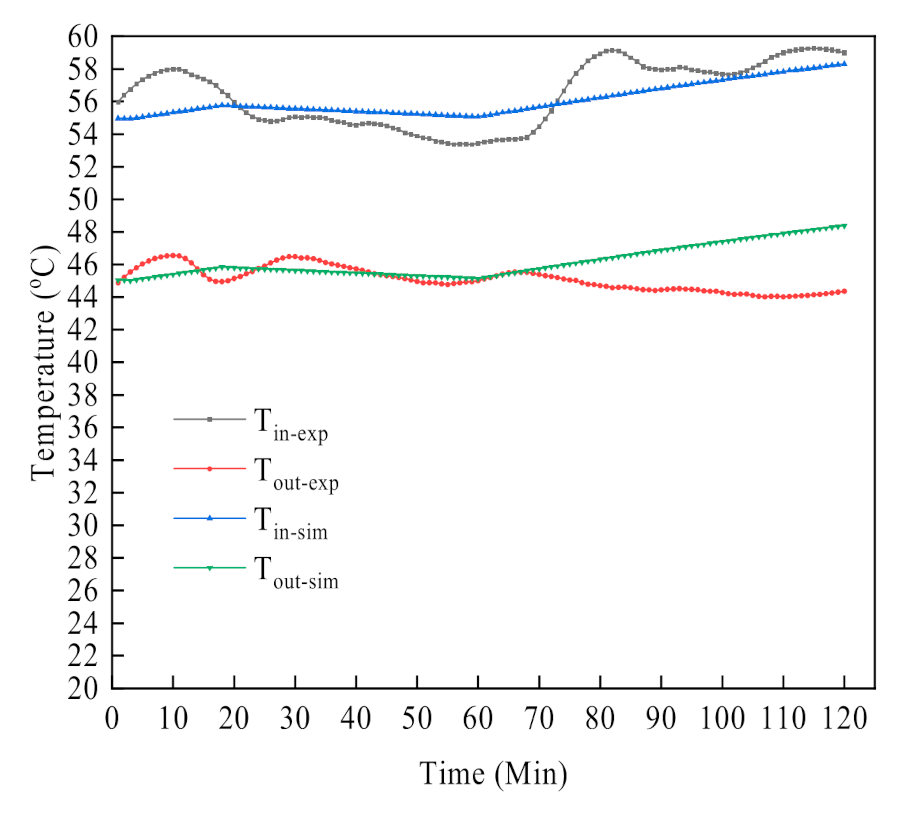
4. Simulation Model Verification

This study uses the experimental results of Qiu [25] to verify the simulation model. The system parameters are consistent with Qiu. The meteorological parameters adopt the typical meteorological year parameters of Nanjing City. The DR inlet temperature and the DR outlet temperature are the verification objects. As shown in Figure 4, the simulated DR inlet temperature ($T_{in-sim}$) has an error of 0.07–6.25% compared with the experimental DR inlet temperature ($T_{in-exp})$, and the average error is 2.36%. Compared with the experimental DR outlet temperature ($T_{out-exp}$), the error of simulated DR outlet temperature ($T_{out-sim}$) is 0.04–10.57%, and the average error is 3.29%.

Compared with the model proposed by Qiu [25], the model proposed in this paper has an additional air-water heat exchanger that connects the BT and DR. The heat exchanger can be regarded as an efficiency device in essence. As shown in Figure 5, when the heat exchanger efficiency is set to 1, the inlet and outlet temperature of the DR is exactly the same as when the heat exchanger is not installed. Set the heat exchanger efficiency to 0.8, 0.6, 0.4, and get the temperature lines of $T_{in-0.8}$, $T_{out-0.8}$ parallel to $T_{in-1}$, $T_{out-1}$. Based on the above comparison and verification results, the simulation system is correct.

5. Results and Discussion

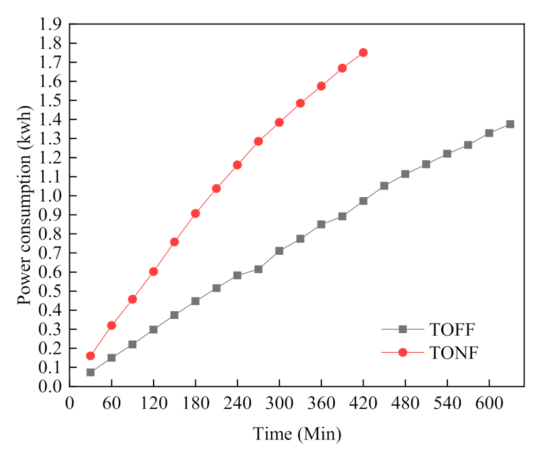
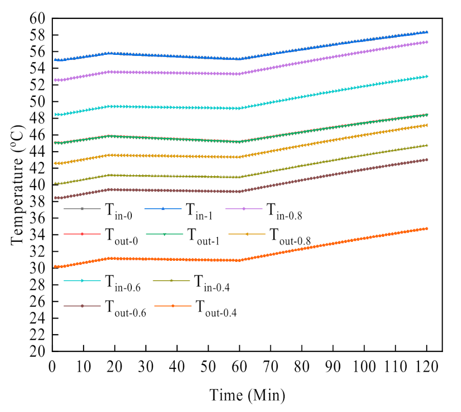
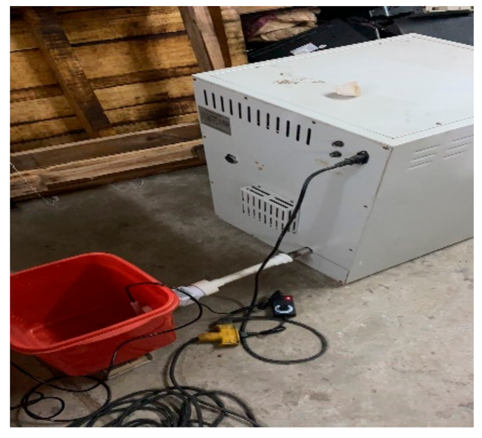
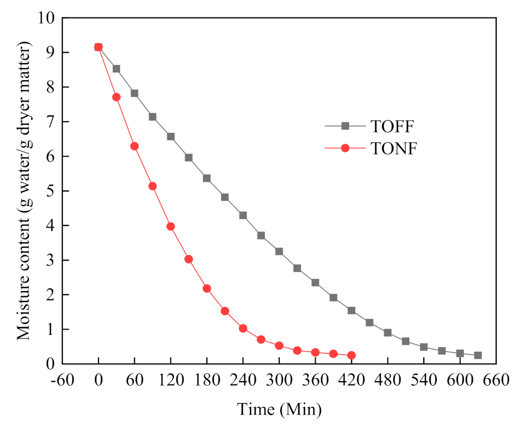
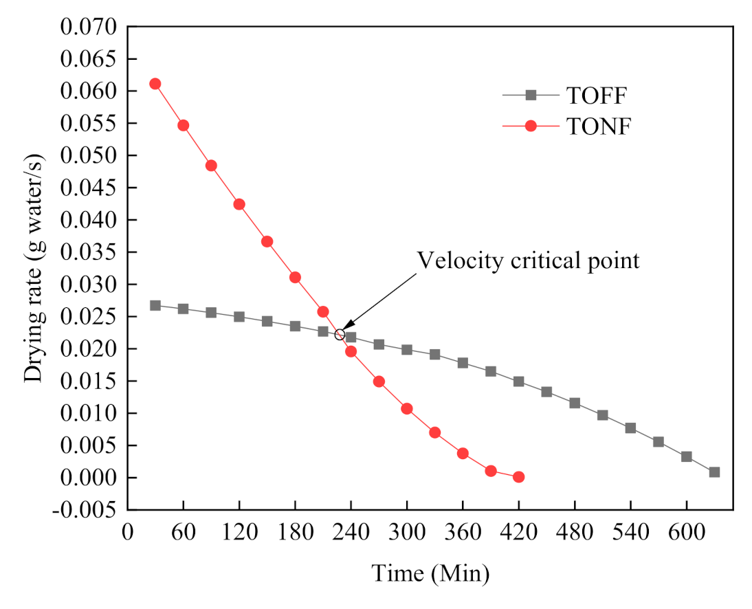
5.1. Variable Air Volume Experiment

In this paper, an electric heating thermostat was modified. On the basis of retaining the original drying room air outlet, a vent was opened, as shown in Figure 6, and a fan added to this vent to perform forced convection for variable air volume experiments and heat recovery. At this time, the original air outlet has become an air inlet, as shown in Figure 7.

In this experiment, 731 g of fresh carrots were dried in two drying modes: the forced convection fan was turned off mode (TOFF) and the forced convection fan was turned on mode (TONF). The flow rate of the fan is $39\mathrm{kg}/\mathrm{h}$. The carrots are equally divided into two plates, and the internal dimensions of the incubator are 0.45 m × 0.45 m × 0.4 m. The initial moisture content of drying is $9.15 \mathrm{g} \mathrm{moisture}/\mathrm{g} \mathrm{dry} \mathrm{matter}$, and the final moisture content is $0.25 \mathrm{g} \mathrm{moisture}/\mathrm{g} \mathrm{dry} \mathrm{matter}$. Therefore, when the weight of dry carrot reaches $0.09 \mathrm{kg}$, the drying process ends. The equipment used in the experiment is shown in

Table 4. Basic Parameters of Typical Cities in Five Climate Zones of China.

Equipment	Measuring Range	Accuracy
Electronic scale	$0–60 \mathrm{kg}$	$1 \mathrm{g}$
Electrical parameter tester	$0–3500 \mathrm{W}$	$0.1 \mathrm{W}$
Anemometer	$0.3–30 \mathrm{m}/\mathrm{s}$	$\pm 3\%$
Temperature Sensor	$-50–200$ °C	0.1 °C
Humidity Sensor	$1–99\%$	$0.1\%$

.

In the experiment, the weight of carrot was measured every half an hour, and the moisture content and drying rate of carrot in the two modes were shown in Figure 8 and Figure 9.

It can be seen from Figure 8 that the drying rate of carrot in the two modes decreases with the increase of time. The drying rate of the TONF mode is 3.5 h faster than that of the TOFF mode, saving 33.3% of the drying time. This is due to the forced convection in the DR, and the humidity is maintained at a low level during the drying process. Natural convection prevents the drying moisture during the drying process from being discharged in time and stays in the DR, making the air humidity close to saturation and inhibiting the drying rate.

It can be seen from Figure 9 that starting from the 4th hour, the drying rate of TONF mode (the forced convection fan was turned on mode) is lower than that of TOFF mode (the forced convection fan was turned off mode). This is because the moisture content of carrots in TONF mode has been reduced to $1.03 \mathrm{g} \mathrm{moisture}/\mathrm{g} \mathrm{dry} \mathrm{matter}$ at this time, and the moisture content of the carrots in TOFF mode corresponds to $4.29 \mathrm{g} \mathrm{moisture}/\mathrm{g} \mathrm{dry} \mathrm{matter}$, the latter is much higher than the former, and the lower moisture content of carrots reduces the drying rate.

It can be seen from Figure 10 that the drying energy consumption in TONF mode (the forced convection fan was turned on mode) is 28.26% higher than that in TOFF mode (the forced convection fan was turned off mode). When TONF mode is switched to TOFF mode in the 4th hour, it can save about 20% of energy compared to TONF mode, and only about 8% higher than TOFF mode. In combination with Figure 8, Figure 9 and Figure 10, we recommend using the mixed mode from TONF to TOFF in the 4th hour (TOCF mode). The drying rate is faster and the energy consumption is low. The following discussion of the article will be based on the TOCF model.

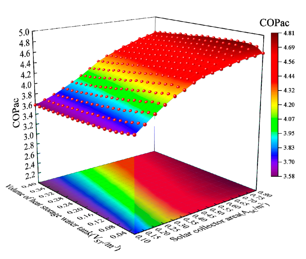
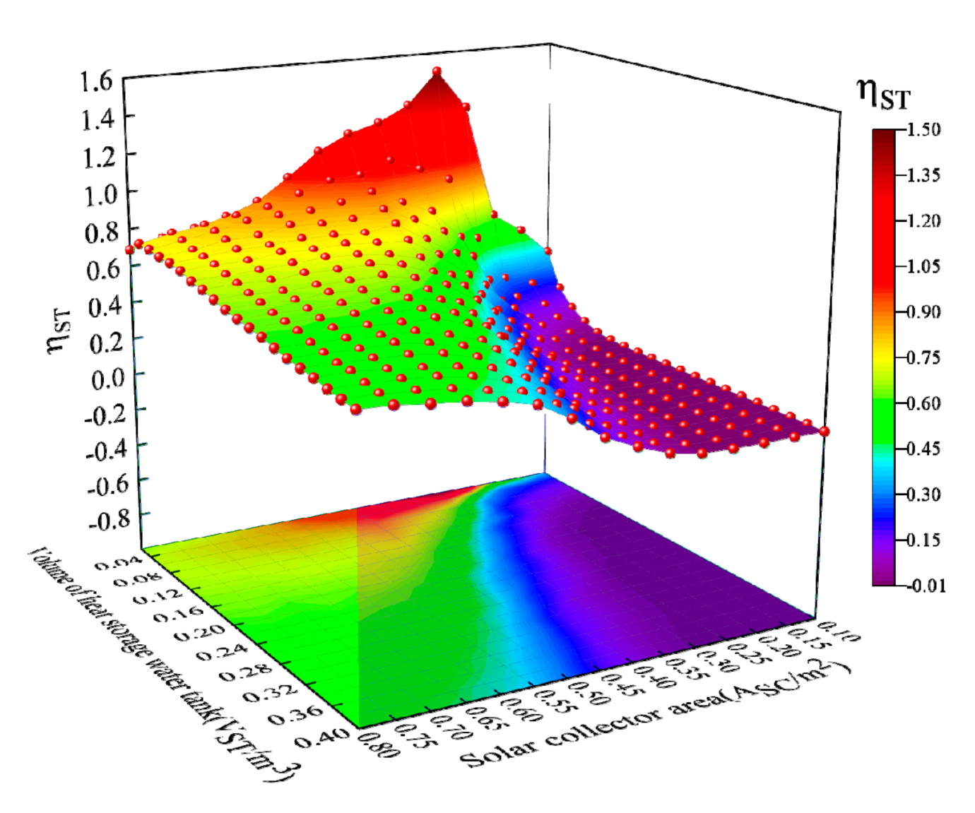
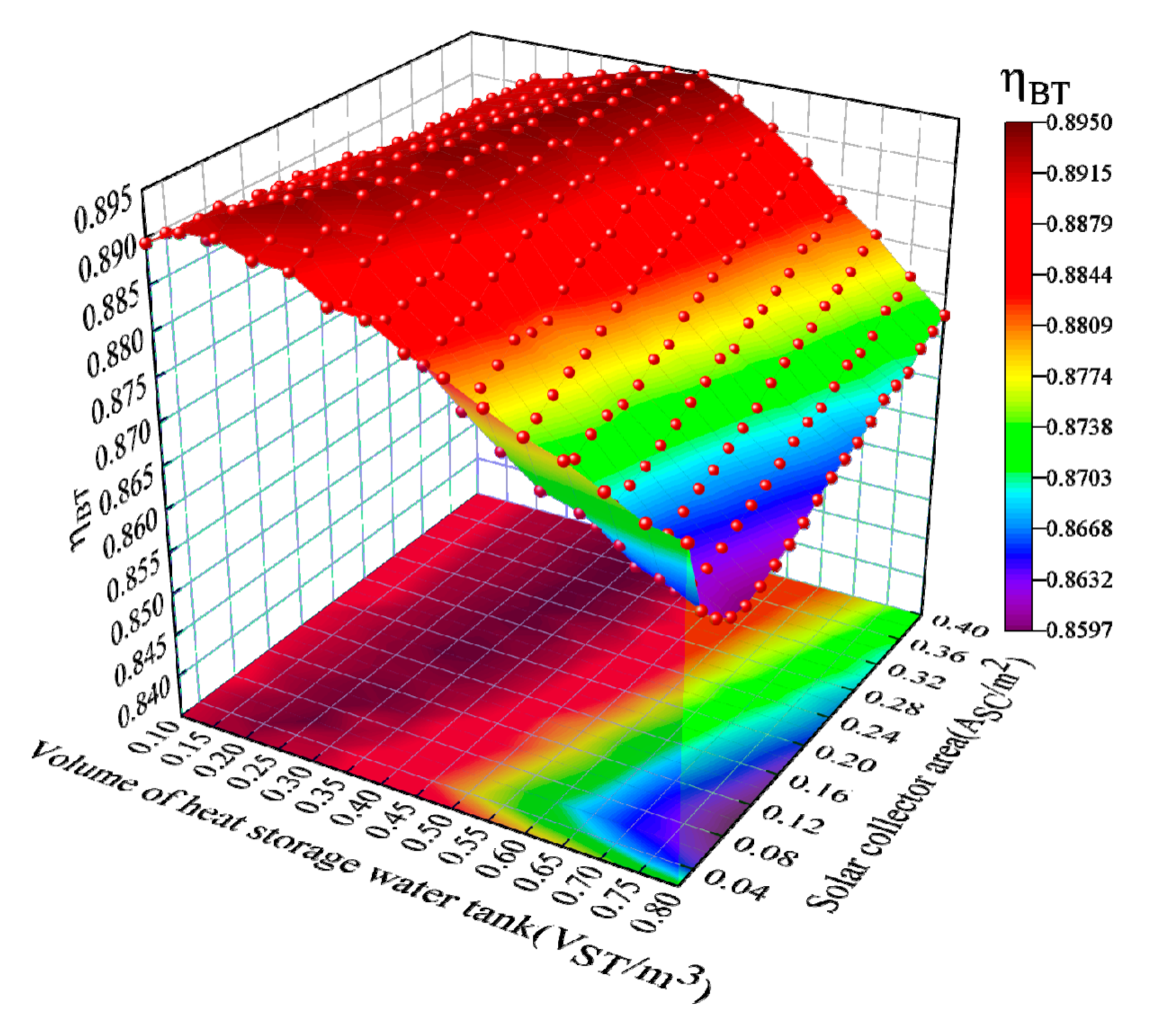
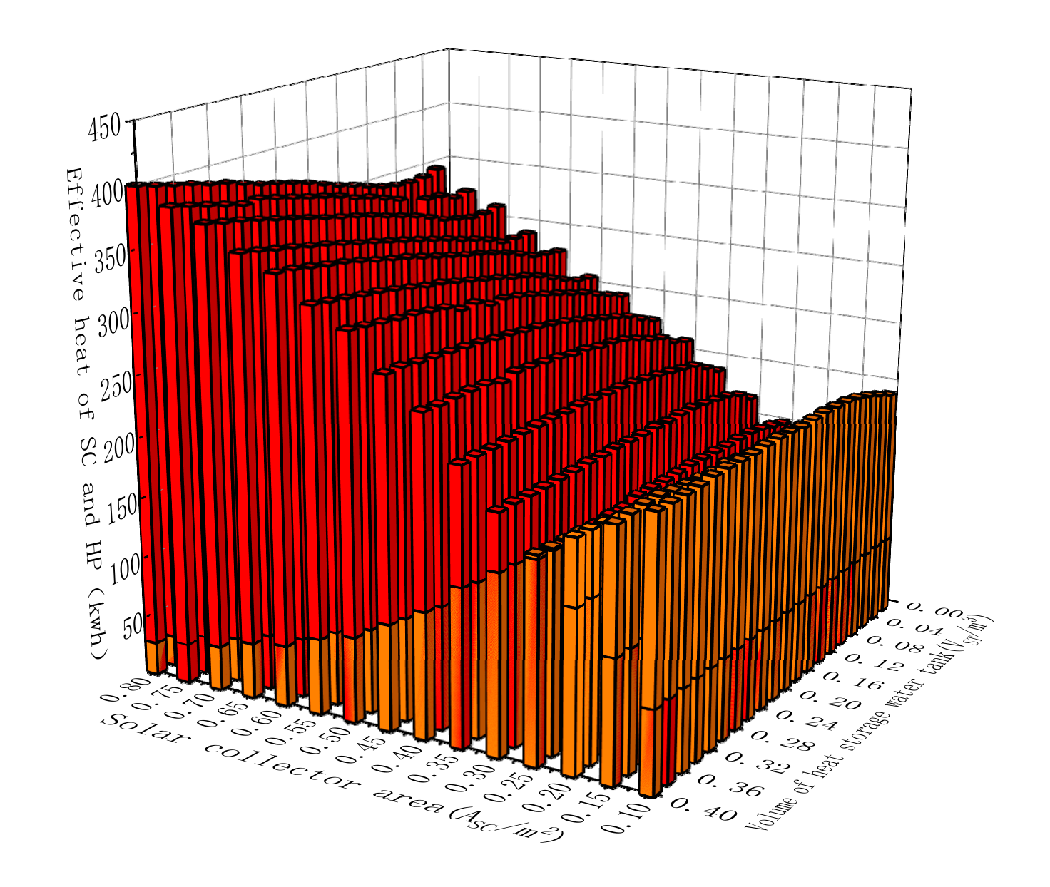
5.2. System Optimization

A solar collector (SC) can effectively improve the overall performance of SCAHP. However, due to high initial investment and different climate conditions in various regions, there are certain difficulties in system design. At the same time, as a key component of the system coupling, a hot water storage tank (ST) also has some difficulties in design. There are few researches on the optimization of heat pump drying system configuration. This research tries to give some suggestions.

As shown in Figure 11, the annual cumulative efficiency of the system $\left(CO{P}_{ac}\right)$ shows an increasing trend with the increase in the area of solar collector $\left(A_{SC}\right)$. This is because as the $A_{SC}$ increases, the proportion of solar heating in the overall heating of the system increases, and the proportion of air-water heat pump (HP) heating is reduced, the total energy consumption of drying room (DR) remains unchanged, the power consumption decreases, and the $CO{P}_{ac}$ increases accordingly. In this configuration, $CO{P}_{ac}$ is 3.571~4.805. As the volume of heat storage water tank $\left(V_{ST}\right)$ increases, $CO{P}_{ac}$ gradually slows down as the $A_{SC}$ increases. When the $V_{ST}$ is $0.02~0.1{ \mathrm{m}}^3$, as the $A_{SC}$ increases, the $CO{P}_{ac}$ with a larger $V_{ST}$ system will always surpass the system with a smaller $V_{ST}$ at a certain point. When the $V_{ST}$ is $0.12~0.4{ \mathrm{m}}^3$, as the $A_{SC}$ increases, the $CO{P}_{ac}$ shows an overall downward trend. This is due to the large $V_{ST}$, the temperature rise of ST is slow, and the heat in the ST cannot be effectively and timely passed to the BT. As a result, on the one hand, the heat collection pump is idling, which increases energy consumption. On the other hand, it cannot effectively reduce the heat supplied by the heat pump and the solar collector cannot be used to the maximum extent, which leads to a decrease in the $CO{P}_{ac}$.

Figure 11 also reveals that when the $A_{SC}$ is $0.1~0.25{ \mathrm{m}}^2$, the $CO{P}_{ac}$ shows a decreasing trend as the $V_{ST}$ increases, and when the $A_{SC}$ is $0.3~0.8{ \mathrm{m}}^2$, the $CO{P}_{ac}$ increases first and then decreases as the $V_{ST}$ increases; this is because the smaller $V_{ST}$ cannot fully release the heat supply potential of the larger $A_{SC}$, and as the $A_{SC}$ increases, the $V_{ST}$ corresponding to the highest value of the system efficiency also increases. When $A_{SC}$ is 0.4, 0.5, and 0.6${\mathrm{m}}^2$ correspond to ST with volumes of 0.04, 0.08, and 0.1${ \mathrm{m}}^3$, respectively, so that the $CO{P}_{ac}$ reaches the corresponding maximum value. In addition, it can be seen from the figure that when the $A_{SC}$ is $0.1~0.4{ \mathrm{m}}^2$, the distance between the lines is relatively sparse. Within this range, as the $A_{SC}$ increases, the $CO{P}_{ac}$ increases rapidly. When the $A_{SC}$ is $0.45~0.8{ \mathrm{m}}^2$, the distance between the lines is relatively dense. In this range, as the $A_{SC}$ increases, the system efficiency increases slowly, which shows that when the $A_{SC}$ is increased to $0.45{ \mathrm{m}}^2$, the system has been mainly heated by the SC, and the HP has played a smaller role. It is recommended to use solar collectors with an area less than $0.45{ \mathrm{m}}^2$ in this system.

In summary, the coupling of the SC and ST is very important. Different $A_{SC}$ require designing a ST of appropriate volume. In order to find this appropriate value, we introduce the surface-to-body ratio (SBR): $SBR=A_{op}/\left(V_{op}+V_{BT}\right)$, Among them, $A_{op}$ and $V_{op}$ respectively represent the $A_{SC}$ and the $V_{ST}$ corresponding to the optimal $CO{P}_{ac}$. $V_{BT}$ is the volume of BT, taking $0.05{ \mathrm{m}}^3$. It can be calculated that the $SBR$ value is concentrated between 3.182~4.091 under the premise of the recommended value.

As shown in Figure 12, when the $V_{ST}$ is $0.02~0.34{ \mathrm{m}}^3$, the ${\eta }_{ST}$ increases first and then decreases as the $A_{SC}$ increases. When the $V_{ST}$ is $0.36~0.4{ \mathrm{m}}^3$, the ${\eta }_{ST}$ shows an increasing trend as the $A_{SC}$ increases. As the $V_{ST}$ increases, the $A_{SC}$ corresponding to the maximum ${\eta }_{ST}$ becomes larger. This is because the larger the $V_{ST}$, the slower the temperature rise, and a larger $A_{SC}$ is required to provide sufficient heat.

Figure 12 also reveals that when the $A_{SC}$ is $0.1~0.55{ \mathrm{m}}^2$, the ${\eta }_{ST}$ shows a decreasing trend as the $V_{ST}$ increases, when the $A_{SC}$ is $0.6~0.8{ \mathrm{m}}^2$, the ${\eta }_{ST}$ will first increase and then decrease as the $V_{ST}$ increases. This is because the $V_{ST}$ is too small compared to the $A_{SC}$, and it cannot store enough solar collector heat. As a result, the heat generated by the SC cannot pass into the BT in time, and the HP needs to be turned on to provide heat to the BT, and the heat generation potential of the SC is not fully utilized. When the $A_{SC}$ is $0.45~0.8{ \mathrm{m}}^2$, the distance between the lines is relatively dense. In this range, as the $V_{ST}$ increases, the ${\eta }_{ST}$ decreases slowly. This shows that when the $A_{SC}$ increases to $0.45{ \mathrm{m}}^2$, it is enough to meet the energy demand of the system. The decrease in the ${\eta }_{ST}$ is mainly caused by the increase in $V_{ST}$. This shows that more heat from the SC is wasted, which confirms the analysis result in Figure 11.

To sum up, take the ${\eta }_{ST}$ as the goal, and based on the effective value of this calculation, the best SBR can be calculated from 1.923 to 4.444, and the $A_{SC}$ corresponding to the maximum ${\eta }_{ST}$ is greater than $0.3{ \mathrm{m}}^2$. It can be seen that the ${\eta }_{ST}$ does not match the overall efficiency of the system. It is recommended to choose a small $V_{ST}$ after selecting the $A_{SC}$, and increase the ${\eta }_{ST}$ to avoid too much heat from the solar collector being wasted. Combining increasing the $A_{SC}$ and $V_{ST}$ will also increase the initial investment, and it is recommended not to take the ${\eta }_{ST}$ as the first choice for system design.

As shown in Figure 13, the ${\eta }_{BT}$ shows a trend of increasing first and then decreasing as the $A_{SC}$ increases; this is because when the $A_{SC}$ is relatively small, the heat of the BT comes from the HP.The HP heats the BT to 65 °C, and during the process of lowering the temperature of the BT, the heat loss is large, which causes the ${\eta }_{BT}$ to be low. As the $A_{SC}$ increases, the heat received by the BT from the SC increases, and the BT will no longer rise to 65 °C frequently, thereby reducing heat loss and improving ${\eta }_{BT}$. With the further increase in the $A_{SC}$, enough heat can be stored in the ST. When the system shuts down at night, the heat from the ST will be transferred to the BT, and then it will interact with the surrounding atmosphere in the BT. The heat exchange causes waste, and the ${\eta }_{BT}$ is gradually reduced. This problem will be solved in a non-stop system.

Figure 13 also reveals that when the $A_{SC}$ is $0.1~0.45{ \mathrm{m}}^2$, the ${\eta }_{BT}$ shows a basically unchanged trend with the increase of $V_{ST}$, during the whole process, the ${\eta }_{BT}$ changes at most by 1.49% and at least 0.44%, which can be ignored. This is because the SC cannot provide sufficient heat for the BT to lose heat at night. When the $A_{SC}$ is $0.5~0.8{ \mathrm{m}}^2$, the ${\eta }_{BT}$ decreases first and then increases as the $V_{ST}$ increases, this is because SC can provide sufficient heat at this time, the ST has a small volume and a high temperature. When it is shut down at night, the ST can provide more heat to the BT, resulting in greater heat loss, as the $V_{ST}$ increases, the temperature of the ST decreases the amount of heat transfer is reduced, the heat loss is also reduced, and the heating efficiency of the BT is gradually improved. In summary, the system configuration required for the maximum efficiency of the BT is different from the system configuration required for the maximum efficiency of the ST.

As shown in Figure 14, the heat provided by the SC shows an increasing trend as the $A_{SC}$ increases. When the $A_{SC}$ is $0.1~0.65{ \mathrm{m}}^2$, the heat supply of the SC shows an increasing trend as the $V_{ST}$ increases, when the $A_{SC}$ is $0.7~0.8{ \mathrm{m}}^2$, the heat supply of SC will decrease first and then increase as the $V_{ST}$ increases. This is because when the $A_{SC}$ is small, as the $V_{ST}$ increases, it can absorb more heat from the SC, and when the $A_{SC}$ is larger, the smaller $V_{ST}$ quickly heats up, which can make better use of the heat recovered from the waste heat, causing the SC to decrease the heat first. The heat provided by the HP shows a decreasing trend as the $A_{SC}$ increases, when the $A_{SC}$ is $0.1~0.25{ \mathrm{m}}^2$, the heat supply of the HP shows an increasing trend as the $V_{ST}$ increases, when the $A_{SC}$ is $0.3~0.8{ \mathrm{m}}^2$, the heat supply of the HP decreases first and then increases as the $V_{ST}$ increases; this is because when the $A_{SC}$ is $0.1~0.25{ \mathrm{m}}^2$, the system mainly relies on the HP heating. As the $A_{SC}$ increases, the system mainly uses the SC for heating, the heat supplied by the HP decreases in the initial stage. Later, as the $V_{ST}$ increases, the ${\eta }_{ST}$ decreases, and the BT needs the HP to provide more heat, which is consistent with the analysis in Figure 12. When the $A_{SC}$ is $0.15~0.35{ \mathrm{m}}^2$, the heat supply ratio of the SC is 34.14~68.03%, which is reasonable.

Based on the above analysis, water tank efficiency and heat supply analysis, we suggest that the $A_{SC}$ of this system is $0.15~0.35{ \mathrm{m}}^2$, the SBR is between 3.2~4.1, and the $V_{ST}$ is $0.02~0.06{ \mathrm{m}}^3$. The recommended values for other climate zones are shown in

Table 5. Recommendation system configuration parameter table of other typical cities.

Name	Recommended SBR	$\mathbf{The} \mathbf{Recommended} \mathbf{Value} \mathbf{of} {\mathit{I}}_{\mathit{S}\mathit{C}} \mathbf{Is} \mathbf{Unchanged} \mathbf{throughout} \mathbf{the} \mathbf{Year} (°)$	$\mathbf{The} \mathbf{Recommended} \mathbf{Value} \mathbf{of} {\mathit{I}}_{\mathit{S}\mathit{C}} \mathbf{Varies} \mathbf{throughout} \mathbf{the} \mathbf{Year} (°)$
Harbin	1.43~2.78	40	50/40 1
Tianjin	1.43~3.57	35	50/30 1
Guangzhou	2.14~3.33	20	40/15 1
Kunming	1.43~2.86	25	45/20 1

¹ a/b means that the $I_{SC}$ is changed to $\mathrm{a}°$ in March, and the $I_{SC}$ is changed to $\mathrm{b}°$ in November until March of the following year.

. The following analysis in this paper will be based on Nanjing, with a $A_{SC}$ of $0.3{ \mathrm{m}}^2$ and a $V_{ST}$ of $0.04{ \mathrm{m}}^3$.

As shown in Figure 15a, the difference in heat supplied by the SC with different $I_{SC}$ in 12 months ranges from 4.83 to 58.27%. October is the month with the smallest difference and June is the month with the largest difference, and the annual average difference is 23.2%. It can be seen that the design of the $I_{SC}$ plays a key role. The annual heat provided by the SC increases first and then decreases with the increase of the $I_{SC}$. When the $I_{SC}$ is $30°$, the total heat provided by the SC throughout the year is the largest. If the SC is designed to have no tilt angle change throughout the year, it is recommended to select a tilt angle of $30°$.

As shown in Figure 15b, when Nanjing is in January to February and November to December, and the $I_{SC}$ is $50°$, the most heat is collected. From March to October, the solar collector can collect the most heat when the $I_{SC}$ is $15°$. Therefore, we recommend changing the $I_{SC}$ twice a year. In March, change the $I_{SC}$ to $50°$, and in November Change the $I_{SC}$ to $15°$ until March of the next year. The configuration parameters of $I_{SC}$ in other cities are shown in Table 5.

5.3. Economic Analysis

The price of material is an important factor affecting the economic analysis of the drying system. According to the heat conservation relationship and calculation, using the life cycle method, the total amount of dried carrot in the system throughout the year is 45.99 kg.

Table 6. Annual revenue diagram of Nanjing drying system.

Year	Annual Net Present Worth	Cumulative Net Present Worth
1	808.17	808.17
2	793.48	1601.65
3	779.05	2380.7
4	764.88	3145.58
5	750.98	3896.56
6	737.32	4633.88
7	723.91	5357.79
8	710.76	6068.55
9	697.83	6766.38
10	685.14	7451.52
11	672.69	8124.21
12	660.46	8784.67
13	648.45	9433.12
14	636.66	10,069.78
15	625.08	10,694.86
16	613.71	11,308.57
17	602.56	11,911.13
18	591.6	12,502.73
19	580.84	13,083.57
20	570.28	13,653.85

shows the annual net present value of Nanjing and the cumulative net present value of the system life. The life cycle method is used to determine the dry payback period of carrot as 5 years. The cumulative net present value is 13,654 yuan respectively.

6. Conclusions

The energy analysis of SCAHP is carried out. The energy coupling relationship of the system in different climate regions is established, and the optimization model of the system is discussed. It can be concluded:

(1)

It is recommended to use the mixed variable air volume mode (TOCF mode) for drying, which can save about 20% of the drying time;

(2)

The system configuration to achieve the maximum system efficiency is not consistent with the system configuration to achieve the maximum water tank efficiency. It is suggested to choose a smaller $V_{ST}$ after selecting $A_{SC}$ to increase the heating efficiency of the ST and improve the system energy utilization rate.

(3)

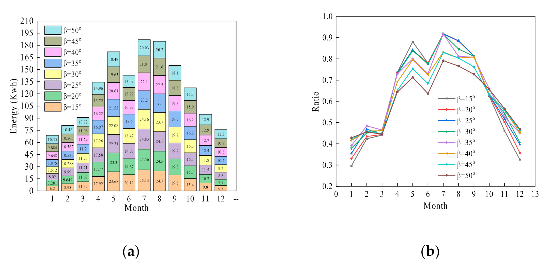
It is suggested that the SBR of SCAHP in Nanjing should be between 3.182 and 4.091, and $I_{SC}$ should be changed twice a year. In March, $I_{SC}$ should be changed to $50°$, and in November, $I_{SC}$ should be changed to $15°$ until the following March. The configuration parameter recommendations for the other cities are shown in Table 5.

(4)

Taking Nanjing as an example to analyze the economy of SCAHP, it can be concluded that the recovery cycle is 5 years, and the system is economically feasible.

References

1. Mohanraj, M.; Belyayev, Y.; Jayaraj, S.; Kaltayev, A. Research and developments on solar assisted compression heat pump systems—A comprehensive review (part-B: Applications). Renew. Sustain. Energy Regen. 2018, 83, 124–155. [Google Scholar] [CrossRef]
2. Hao, W. Theoretical and Experimental Research on the Dual Working Medium Drying System Based on Solar Energy Thermal Utilization. Ph.D. Thesis, Shandong University, Jinan, China, 2020. [Google Scholar]
3. Mujumdar, A.S. Handbook of Industrial Drying, 3rd ed.; CRC Press: Boca Raton, FL, USA, 2006; pp. 2–29. [Google Scholar]
4. Colak, N.; Hepbasli, A. A review of heat pump drying: Part 1—Systems, models and studies. Energy Convers. Manag. 2009, 50, 2180–2186. [Google Scholar] [CrossRef]
5. Lawton, J. Drying: The role of heat pumps and electromagnetic fields. Phys. Technol. 1978, 9, 214–220. [Google Scholar] [CrossRef]
6. Queiroz, R.; Gabas, A.L.; Telis, V.R.N. Drying kinetics of tomato by using electric resistance and heat pump dryers. Dry Technol. 2004, 22, 1603–1620. [Google Scholar] [CrossRef]
7. Claussen, I.C.; Ustad, T.S.; Strmmen, I.; Walde, P.M. Atmospheric freeze drying—A review. Dry Technol. 2007, 25, 947–957. [Google Scholar] [CrossRef]
8. Krokida, M.K.; Kiranoudis, C.T.; Maroulis, Z.B.; Marinos-Kouris, D. Drying related properties of apple. Dry Technol. 2000, 18, 1251–1267. [Google Scholar] [CrossRef]
9. Perera, C.O.; Rahman, M.S. Heat pump dehumidifier drying of food. Trends Food Sci. Technol. 1997, 8, 75–79. [Google Scholar] [CrossRef]
10. Prasertsan, S.; Saen-saby, P. Heat pump drying of agricultural materials. Dry Technol. 1998, 16, 235–250. [Google Scholar] [CrossRef]
11. Rossi, S.; Neues, L.; Kicokbusch, T. Thermodynamic and energetic evaluation of a heat pump applied to the drying of vegetables. Drying 1992, 92, 1475–1478. [Google Scholar]
12. Hodgett, D. Efficient drying using heat pumps. Chem. Energy 1976, 311, 510–512. [Google Scholar]
13. Geeraert, B. Air drying by heat pumps with special reference to timber drying. In Heat Pumps and Their Contribution to Energy Conservation, 1st ed.; Camatini, E., Kester, T., Eds.; Springer: Berlin/Heidelberg, Germany, 1976; pp. 219–246. [Google Scholar]
14. Hawlader, M.N.A.; Perera, C.O.; Tian, M.; Yeo, K.L. Drying of guava and papaya: Impact of different drying methods. Dry Technol. 2006, 24, 77–87. [Google Scholar] [CrossRef]
15. Sun, Z.; Wang, Q.; Xie, Z.; Liu, S.; Su, D.; Cui, Q. Energy and exergy analysis of low GWP refrigerants in cascade refrigeration system. Energy 2019, 170, 1170–1180. [Google Scholar] [CrossRef]
16. Wang, N.; Ye, Q.; Chen, L.; Zhang, H.; Zhong, J. Improving the economy and energy efficiency of separating water/acetonitrile/isopropanol mixture via triple-column pressure-swing distillation with heat-pump technology. Energy 2021, 215, 119–126. [Google Scholar] [CrossRef]
17. Li, X.; Wang, D. Study on thermodynamic characteristics of multi-unit parallel heat pump drying System. Chin. J. Refrig. Technol. 2018, 38, 61–67. [Google Scholar]
18. Hasan Ismaeel, H.; Yumrutaş, R. Investigation of a solar assisted heat pump wheat drying system with underground thermal energy storage tank. Sol. Energy 2020, 199, 538–551. [Google Scholar] [CrossRef]
19. Fudholi, A.; Sopian, K.; Ruslan, M.H.; Alghoul, M.A.; Sulaiman, M.Y. Review of solar dryers for agricultural and marine products. Renew. Sustain. Energy Regen. 2010, 14, 1–30. [Google Scholar] [CrossRef]
20. El-Sebaii, A.A.; Shalaby, S.M. Solar drying of agricultural products: A review. Renew. Sustain. Energy Regen. 2012, 16, 37–43. [Google Scholar] [CrossRef]
21. Huilong, L.; Jinhui, P.; Libo, Z.; Shenghui, G. Performance analysis of a solar energy drying system in conjunction with air source heat pump. Acta Energy Sol. Sin. 2012, 33, 963–967. [Google Scholar]
22. Rahman, S.M.A.; Saidur, R.; Hawlader, M.N.A. An economic optimization of evaporator and air collector area in a solar assisted heat pump drying system. Renew. Sustain. Energy Regen. 2013, 76, 377–384. [Google Scholar] [CrossRef]
23. Koşan, M.; Demirtaş, M.; Aktaş, M.; Dişli, E. Performance analyses of sustainable PV/T assisted heat pump drying system. Sol. Energy 2020, 199, 657–672. [Google Scholar] [CrossRef]
24. Laszlo, L. Solar drying. In Handbook of Industrial Drying, 3rd ed.; Mujumdar, A.S., Ed.; CRC Press: Boca Raton, FL, USA, 2006; Volume 2, pp. 304–346. [Google Scholar]
25. Qiu, Y.; Li, M.; Hassanien, R.H.E.; Wang, Y.; Luo, X.; Yu, Q. Performance and operation mode analysis of a heat recovery and thermal storage solar-assisted heat pump drying system. Sol. Energy 2016, 137, 225–235. [Google Scholar] [CrossRef]
26. Wang, Y.; Li, M.; Qiu, Y.; Yu, Q.; Luo, X.; Li, G. Performance analysis of a secondary heat recovery solar-assisted heat pump drying system for mango. Energy Explor. Exploit. 2019, 37, 1377–1387. [Google Scholar] [CrossRef]
Figure 1. Schematic diagram of SCAHP.
Processes 09 01118 g001
Figure 2. (a) SCAHP operation logic, part 1: the control logic of SCAHP except for the waste heat recovery module. (b) SCAHP operation logic, part 2: the control logic of the waste heat recovery module.
Processes 09 01118 g002aProcesses 09 01118 g002b
Figure 3. TRNSYS model of SCAHP.
Processes 09 01118 g003
Figure 4. Diagram of comparison and verification of inlet and outlet temperatures of the DR.
Processes 09 01118 g004
Figure 5. Diagram of verification of the heat exchanger in TRNSYS, essentially an efficiency unit.
Processes 09 01118 g005
Figure 6. Schematic diagram of adding vent to the thermostat.
Processes 09 01118 g006
Figure 7. Schematic diagram of installing fan on vent.
Processes 09 01118 g007
Figure 8. Changes of carrot moisture content with drying time.
Processes 09 01118 g008
Figure 9. Changes of carrot moisture drying speed with time.
Processes 09 01118 g009
Figure 10. Changes of carrot drying power consumption over time.
Processes 09 01118 g010
Figure 11. Diagram of COPac changes as ASC and VST change.
Processes 09 01118 g011
Figure 12. Diagram of ηST changes as ASC and VST change.
Processes 09 01118 g012
Figure 13. Diagram of ηBT changes as ASC and VST change.
Processes 09 01118 g013
Figure 14. Diagram of the effective heat provided by the SC and HP as ASC and VST change.
Processes 09 01118 g014
Figure 15. (a) Schematic diagram of the energy that can be provided by the SC throughout the year under different ISC. (b) Schematic diagram of the ratio of heat provided by the SC in the total heat supply of the system under different ISC.
Processes 09 01118 g015