Introducing Parameter Clustering to the OED Procedure for Model Calibration of a Synthetic Inducible Promoter in S. cerevisiae

Abstract

In recent years, synthetic gene circuits for adding new cell features have become one of the most powerful tools in biological and pharmaceutical research and development. However, because of the inherent non-linearity and noisy experimental data, the experiment-based model calibration of these synthetic parts is perceived as a laborious and time-consuming procedure. Although the optimal experimental design (OED) based on the Fisher information matrix (FIM) has been proved to be an effective means to improve the calibration efficiency, the required calculation increases dramatically with the model size (parameter number). To reduce the OED complexity without losing the calibration accuracy, this paper proposes two OED approaches with different parameter clustering methods and validates the accuracy of calibrated models with in-silico experiments. A model of an inducible synthetic promoter in S. cerevisiae is adopted for bench-marking. The comparison with the traditional off-line OED approach suggests that the OED approaches with both of the clustering methods significantly reduce the complexity of OED problems (for at least 49.0%), while slightly improving the calibration accuracy (11.8% and 19.6% lower estimation error in average for FIM-based and sensitivity-based approaches). This study implicates that for calibrating non-linear models of biological pathways, cluster-based OED could be a beneficial approach to improve the efficiency of optimal experimental design.

1. Introduction

For decades, mathematical models have played a substantial role in biological and pharmaceutical researches as a tool to quantitatively characterise the behaviour of cells. Because of the natural non-linearity of cell responses and biological noise, the experiment-based model calibration is commonly a laborious and time-consuming procedure [1,2,3,4]. To address this problem, the optimal experimental design (OED) is developed to improve the calibration efficiency and accuracy [5,6].

Fisher information matrix (FIM) is the foundation of many model-driven OED methods [7,8,9]. The benefits of FIM-based OED have been proved in many previous biochemical studies with cells [10,11,12]. For example, in a recent work from Bandara et al. [3] with a case study of model calibration for a synthetic orthogonal promoter, compared to traditional experimental designs including random stimuli, FIM-based OED achieved a 60% smaller average relative estimation error of all the parameters. According to the Cramer-Rao inequality [13,14], the FIM gives the lower bound on the variance of parameter estimated base on a particular experiment. In other words, the FIM defines a mapping from the experimental design space to the space of estimation accuracy, and the OED is the process that searches in the design domain to maximise the estimation accuracy.

Although the FIM-based OED have improved the model calibration experiments in many works, previous studies also expressed some concerns about the current FIM-based OED approaches in future applications. First, as noticed by many researchers, the OED procedure may require considerable computational effort, particularly for non-linear models [3,7,15,16,17,18]. Considering the current trend of increasing model complexity and the expanding feasible space for experimental design, it would be an increasingly critical problem [17]. Some previous studies have provided algorithms to speed up the FIM evaluation for non-linear models, some of the commonly adopted approaches are Markov Chain Monte Carlo (MCMC [19]), Adaptive Gaussian Quadrature (ACQ [20]), and simplified FIM with assumptions of the observation distribution [21,22]. Although these methods may avoid the exponentially growing number of model evaluations (i.e., the sampling number) [23], by definition the calculation complexity of FIM is still proportional to or higher than $N_{\theta }^2$ [22,24].

Another concern is the accuracy trade-offs between the accuracy of different parameters. A commonly adopted method is introducing a scalar objective criterion that quantifies the overall accuracy, such as the D-optimality ($det\left(FIM\right)$, product of the estimation variances), A-optimality ($tr\left(FIM\right)$, sum of the estimation variances), and E-optimality ($min\left({\lambda }_{FIM}\right)$, the worst estimation accuracy) [25,26,27]. Nevertheless, a widely held view is that these criteria have their strengths and weaknesses in practices, so the concern changes to the trade-offs between the criteria [21,28,29]. Fundamentally, this problem is caused by the inherent property of the models and the selection of parameters to calibrate.

To address these limitations in FIM-based OED, this paper borrows the concept of parameter clustering from relative studies [17,30,31,32,33,34]. This method is originally proposed to guide the model calibration for the case that only a subset of model parameters can be calibrated because of identifiability issues (the problem that model gives identical outputs with non-unique parameter value sets) [35,36]. Based on the effect pattern that each parameter values have on the model prediction, the parameters with similar patterns are more likely to cause the identifiability problem and shall be grouped into a common cluster. By selecting one parameter from each cluster to estimate and fixing the rest, the identifiability problem is less likely to appear and the overall variance of the estimation shall be reduced. The complexity for evaluating the FIM matrix is $O\left(N_{\theta }^2\right)$ ($N_{\theta }$ is the number of parameters to focus). Considering accuracy trade-offs (it varies with models and is difficult to quantify, but generally increase with model size [23]), the complexity growth for FIM-based OED could be faster than $O\left(N_{\theta }^2\right)$ [21,24].

This paper explores two approaches that improve the OED procedure by adopting parameter clustering and compares the calibration accuracy to the traditional OED method. As a benchmark, the study considers optimising an experiment sequence for calibrating a model of a synthetic inducible promoter designed by Gnügge et al. [37]. Different from the previous applications of parameter clustering [17,32], the clustering results are not used to establish identifiable parameter sets. Instead, in each sub-experiment of the sequence, the OED is carried out to optimise the estimation accuracy for only one parameter cluster (so the computational cost is reduced), and the number of sub-experiments corresponds to the cluster number. In-silico experimental data are generated and used for the final model calibration. The estimation accuracy of these methods are compared to randomised experimental design and the traditional OED approach, which optimise the overall accuracy for all the parameters in each sub-experiment. The analysis shows that both of the approaches significantly reduce the complexity of OED problems while remaining or even slightly improving the calibration accuracy.

2. Materials and Methods

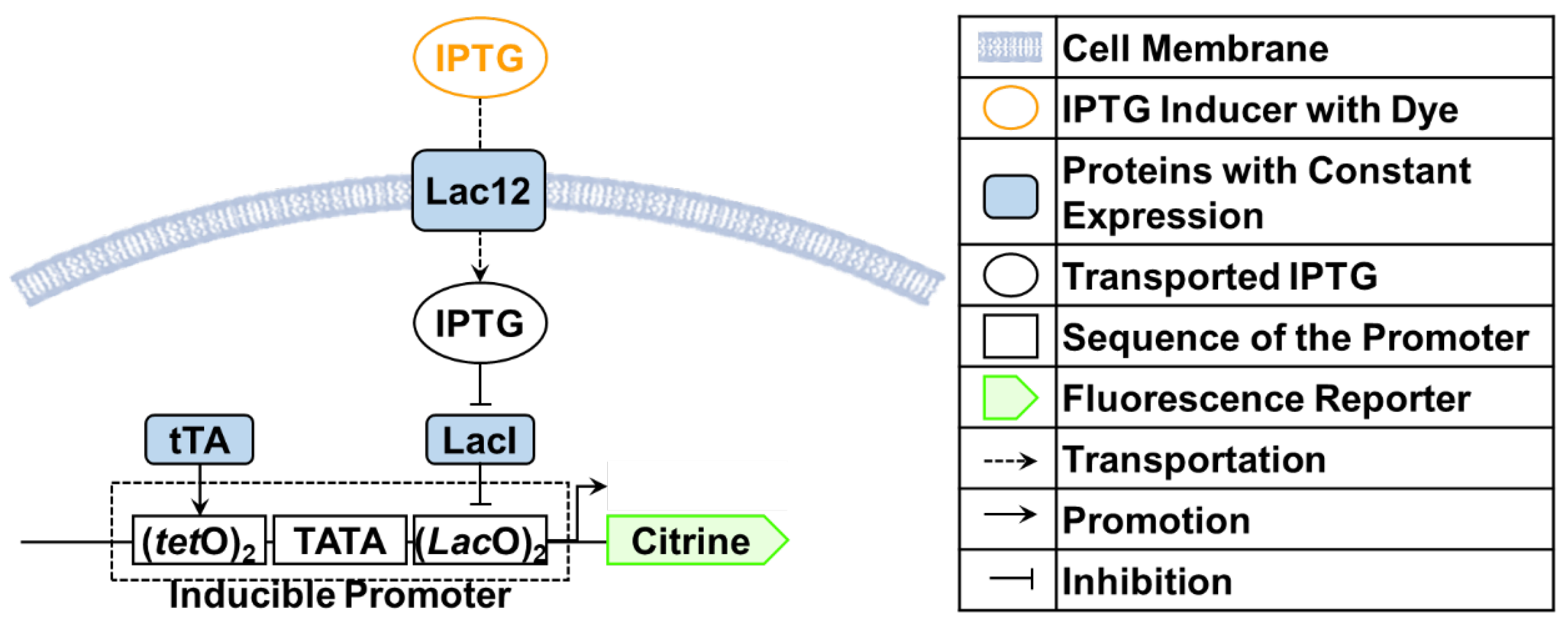
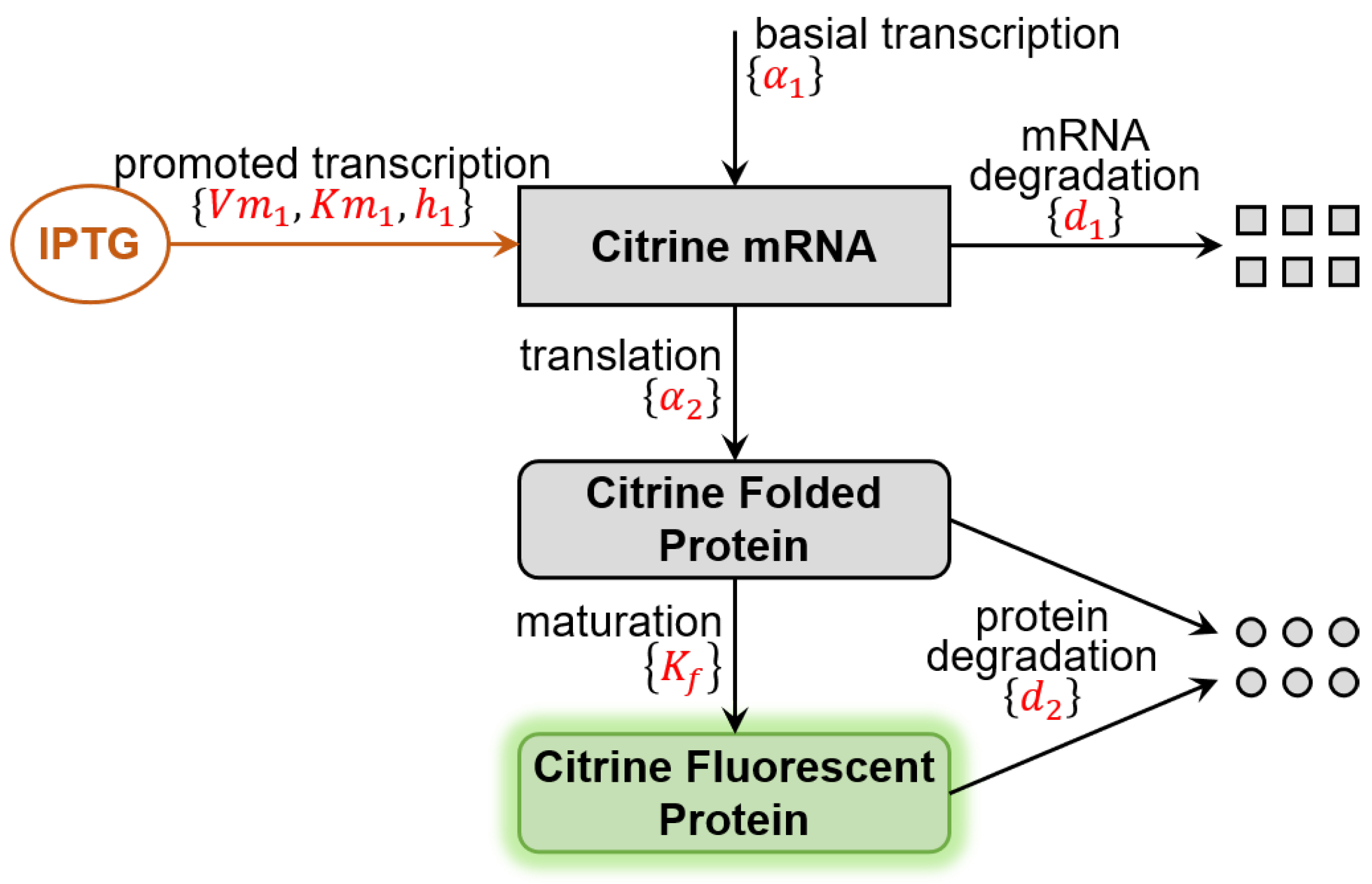
2.1. Benchmark Model for Calibration

As introduced in the previous section, the work of this paper uses a model of a synthetic inducible promoter in S. cerevisiae (yeast) as a benchmark. This model is selected because it is in the form of ordinary differential equations (ODE), a very representative mathematical expression for modelling dynamic biological systems [38,39,40,41], and it contains a Hill function which is a classic non-linear mechanism in the studies of enzyme kinetics and general biochemistry [16,42,43]. Moreover, the parameter values and feasible ranges are supported by previous wet-lab experiments [37,44,45,46,47,48], which further strengthens its authenticity and representativeness.

As shown in Figure 1, the synthetic promoter regulates the expression level of the fluorescent reporter protein (Citrine) according to the extracellular concentration of the inducer (isopropyl $\beta$-D-thiogalactoside, IPTG). When IPTG is added to cell culture, it is transported into yeast cells by protein Lac12 and bounds to LacI, which is a repressor that inhibits the transcription of Citrine. In other words, IPTG indirectly promotes the expression of Citrine by relieving the inhibition of LacI upon LacO.

The mathematical model (Equation (1)) is established according to the famous central dogma, the protein maturation mechanism, and the degradation of messenger RNA and proteins. Figure 2 visualises the modelled reactions and how the model parameters quantitatively describe these reactions. Notice that some of the reactions are not included in the model, such as IPTG bounding to LacI, and LacI bounding to LacO. It is because their reaction rates are significantly faster than the other ones, and dynamic equilibrium can be achieved in few minutes (while the sampling period in practice is 5 min). The overall effects of these reactions are described as the Hill function in $\left[{Cit}_{mRNA}\right]$’s equation, which is a typical approach in biological modelling [16,43].

$$\left\{\begin{array}{cc}\frac{d}{dt}\left[{Cit}_{mRNA}\right]\hfill & ={\alpha }_1+{Vm}_1\frac{{\left[IPTG\right]}^{h_1}}{{\left[IPTG\right]}^{h_1}+{\left({Km}_1\right)}^{h_1}}-d_1\left[{Cit}_{mRNA}\right]\hfill \\ \frac{d}{dt}\left[{Cit}_{foldedP}\right]\hfill & ={\alpha }_2\left[{Cit}_{mRNA}\right]-(d_2+K_f)\left[{Cit}_{foldedP}\right]\hfill \\ \frac{d}{dt}\left[{Cit}_{fluo}\right]\hfill & =K_f\left[{Cit}_{foldedP}\right]-d_2\left[{Cit}_{fluo}\right]\hfill \end{array}\right.$$

(1)

where $\left[{Cit}_{mRNA}\right]$, $[{Cit}_{foldedP}$, and $\left[{Cit}_{fluo}\right]$ are the concentrations (in arbitrary unit, $A.U.$) of the messenger RNA, folded Citrine protein and matured Citrine protein that is fluorescent (observable); $\left[IPTG\right]$ is the extracellular concentration (in $molar$) of IPTG. This model has eight parameters: ${\alpha }_1$ is the basal transcription rate ($A.U.$/min); $V{m}_1$ is the maximum promoted transcription rate ($A.U.$/min); $h_1$ is the Hill coefficient (dimension less); $K{m}_1$ is the Michaelis Menten coefficient ($molar$); $d_1$ is the mRNA degradation rate (min${}^{-1}$); ${\alpha }_2$ is the translation rate (min${}^{-1}$); $d_2$ is the protein degradation rate (min${}^{-1}$); $k_f$ is the maturation rate (min${}^{-1}$). Because of identifiability issues, ${\alpha }_2$ is fixed to the current best estimation during the calibration (this parameter is unidentifiable with the overall scale of ${\alpha }_1$ and $V{m}_1$). The other seven parameters are structurally identifiable.

2.2. Optimal Experimental Design Based on the Fisher Information Matrix

As mentioned in the Introduction, Fisher information matrix (FIM) is a classic mathematical tool for guiding the optimal experimental design. This theory can be traced back to the 1930s from R.A.Fisher [49]. Under the assumption that the observation at each sampling time follows a multivariate normal distribution (a commonly adopted assumption in biology), the FIM as a function of parameter set $\theta$ and stimuli design u can be defined as Equation (2) [21,22]:

$$FI{M}_{i,j}(\theta ,u)=\sum _{s=1}^{N_s^j}{\frac{\partial y_s(\theta ,u)}{\partial {\theta }_i}}^T{\sigma }^{-1}\frac{\partial y_s(\theta ,u)}{\partial {\theta }_j}$$

(2)

where i and j are parameter indexes (for example, in this case i and j are integers between 1 and 7), $N_s^j$ is the number of sampling times in the experiment, s is the index of sampling time, and $d{y}_s^j/d{\theta }_i$ is the derivative of the model prediction of the observable y at the specified sampling index s corresponds to a small value change in the specified parameter ${\theta }_i$, $\sigma$ is the matrix of the variance in the observation. For the cases that only involves one observable, $\sigma$ degenerates to a scalar. For multiple observable cases, the diagonal elements of $\sigma$ are the variance of each observable, and the off-diagonal elements are the co-variances between observations. The units of y and $\sigma$ depends on the observations. In this study, y is the light signal intensity in Citrine channel (in arbitrary unit, $A.U.$), which is proportional to the concentration of Citrine reporter in cells. The FIM is an $N_{\theta }\times N_{\theta }$ matrix where $N_{\theta }$ i the number of parameters under consideration. By introducing the assumptions, this approach reduces the computational complexity of FIM evaluation from exponential growth [23] down to $O\left(N_{\theta }^2\right)$[24]. In this bench-marking study, the evaluation of FIM for all the parameters ($N_{\theta }=7$) requires at least 96% more computing power than the FIM for a parameter cluster ($N_{\theta }\le 5$).

The Cramer-Rao inequality which describes how the FIM can give a lower-bound of the estimation of each parameter (Equation (3), [22]):

$$Va{r}_i(\theta ,u)\ge FI{M}_{i,i}{(\theta ,u)}^{-1}$$

(3)

The equation holds when the error in estimation forms a multivariate Gaussian distribution.

For optimising the accuracy of multiple parameters and leads to one experimental design, a generally adopted approach is to define a scalar criterion to represent the overall accuracy for all these parameters Common criteria includes: D-optimality (maximise the determinant of FIM), A-optimality (maximise the trace of FIM), and E-optimality (maximise the smallest eigenvalues of FIM) [25,26,27]. In this study, D-optimality is adopted because it provides a more smooth design-criterion mapping, and also more sensitive to identifiability issues (this criterion would always be 0 if there are unidentifiable parameters).

2.3. Parameter Clustering Based on Sensitivity Vectors

This approach bases on the sensitivity vectors of the model-predicted observable values corresponding to changes in each parameter value under different input stimuli patterns. The aim is to find the parameters which share similar stimuli-sensitivity patterns. There are three commonly adopted metrics for describing the sensitivity information in experiments [50]: mean squared sensitivity ($d_{msqr}$), mean absolute sensitivity ($d_{mabs}$), and mean sensitivity ($d_{mean}$). This study selected the mean squared sensitivity ($d_{msqr}$) because the sign of sensitivity does not matter the experimental informativeness (for example, if only ${\theta }_1-{\theta }_2$ is identifiable, the sensitivity values of these two parameters would always be opposite to each other and they should be grouped in one cluster), and this metric gives more weights to the sample points with higher sensitivity levels. The mathematical expression of this metric is given as Equation (4).

$$d_{msqr,i}^j=\sqrt{\frac{1}{N_s^j}\sum _{s=1}^{N_s^j}{\left(\frac{d{y}_s^j}{d{\theta }_i}\right)}^2}$$

(4)

where j is the experiment index, i is the parameter index, $N_s^j$ is the number of sampling times in the ith experiment, s is the index of sampling time, and $d{y}_s^j/d{\theta }_i$ is the derivative of the model prediction of the observable y at the specified sampling index s corresponds to a small value change in the specified parameter ${\theta }_i$.

Once the sensitivity is defined, the vectors of sensitivity for model parameter ${\theta }_i$ in $N_j$ number of experiments can be obtained in the form as Equation (5).

$$v_i=\left[d_{msqr,i}^1,d_{msqr,i}^2,\dots ,d_{msqr,i}^{N_j}\right]$$

(5)

Considering two parameters ${\theta }_1$ & ${\theta }_2$ and corresponding sensitivity vectors $v_1$ and $v_2$, the level of dissimilarity can be quantified by cosine distance defined as Equation (6), this metric is also used for parameter clustering in some previous studies [17,51]. It is adopted because this distance does not change with parameter units. Most of the other distance metrics (e.g., Euclidean distance, city block distance, and Minkowski distance) do not have such property.

$$d_{cosine}(v_1,v_2)=1-\frac{v_1{v_2}^T}{\sqrt{v_1{v_1}^T{v}_2{v_2}^T}}=1-corr([v_1,-v_1],[v_2,-v_2])$$

(6)

The final step is to cluster the parameters according to the similarity of the sensitivity vectors. Similar to some previous studies [52,53], this study adopts the Hierarchical algorithm [54]. K-means is another option for this task [55,56], although it is slightly less robust (the clustering result may change with the randomised initiation). The gap criterion is used to determine the clustering numbers [57], and the Silhouette criterion is an alternative option [58]. For calculating the distances between clusters, UPGMA (Unweighted average distance between cluster elements) is used. The advantages of UPGMA are its robustness and compatibility with non-Euclidian distances [52,59].

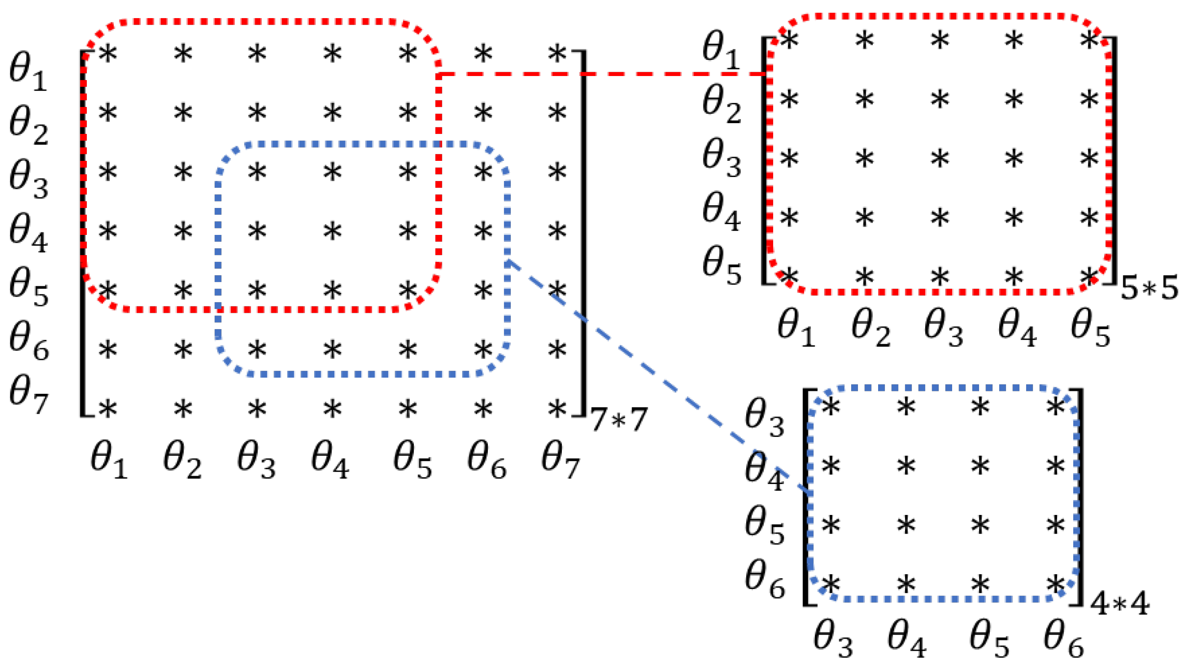
2.4. Parameter Clustering Based on FIM

A newly proposed approach from this paper bases on the Fisher information matrices (FIMs) of experiments. This clustering procedure is equivalent to solving a non-linear optimisation problem. This task is looking for the optimal clustering result so that the patterns of informativeness of fitting parameter clusters with different experimental designs get maximally differed. In other words, ideally, there would be some experimental designs particularly efficient for estimating one parameter cluster, and some other designs are efficient for another cluster.

From the description above, the clustering procedure seems to involve complex and repeated evaluations of the FIM for estimating different parameter clusters, but in fact, it can be obtained with a simple calculation that does not need to repeat. For each experiment, a “full” FIM can be calculated for the case of fitting all the parameters. As introduced in Section 2.2, FIM is an $N_{\theta }\times N_{\theta }$ matrix where $N_{\theta }$ is the number of parameters to fit. FIM has an important property that for the case of fitting a subset of parameters with the same experimental design, the new FIM is exactly the corresponding sub-part of the “Full” FIM (Figure 3). Therefore, the FIM for all the parameters contains the estimation accuracy information to fit any subgroups of the parameters.

For a specific parameter clustering result, the determinant of the FIM (i.e., D-optimality [4,29]) can be calculated for each parameter subset in every experimental design. As shown in Equation (7), this defines the vectors of the informativeness in a similar form as the sensitivity vectors in Section 2.3:

$$V_i=\left[D_i^1,D_i^2,\dots ,D_i^{N_j}\right]$$

(7)

where i is the index of parameter cluster (not the index of a parameter), $D_i^1$ is the D-optimality for fitting the ith parameter cluster with the 1st experimental design, $N_j$ is the total number of experimental designs. The task is to maximise a criterion that quantifies the difference between the informativeness vectors for different parameter clusters by adjusting the parameter clustering.

To the best of author’s knowledge, there are no previous researches that cluster the parameters according to the FIM metrics. There are some commonly used clustering evaluation criteria, such as Gap [57], Silhouette [58], Calinski-Harabasz [60], and Davies-Bouldin [61]. However, they are all based on the within-to-between cluster distances, which does not work for the FIM based clustering. As there is only one vector for one cluster, there is no “within-cluster distance” or information about the variance within the cluster. Therefore, in this task, the smallest cosine distance between informativeness vectors is chosen as the criterion, and this value should be as large as possible. A few other options have also been tried: determination coefficients instead of cosine distance, and averaged between-cluster distance instead of the smallest distance. The results show that the selected method is more robust and better balances informativeness and clustering complexity.

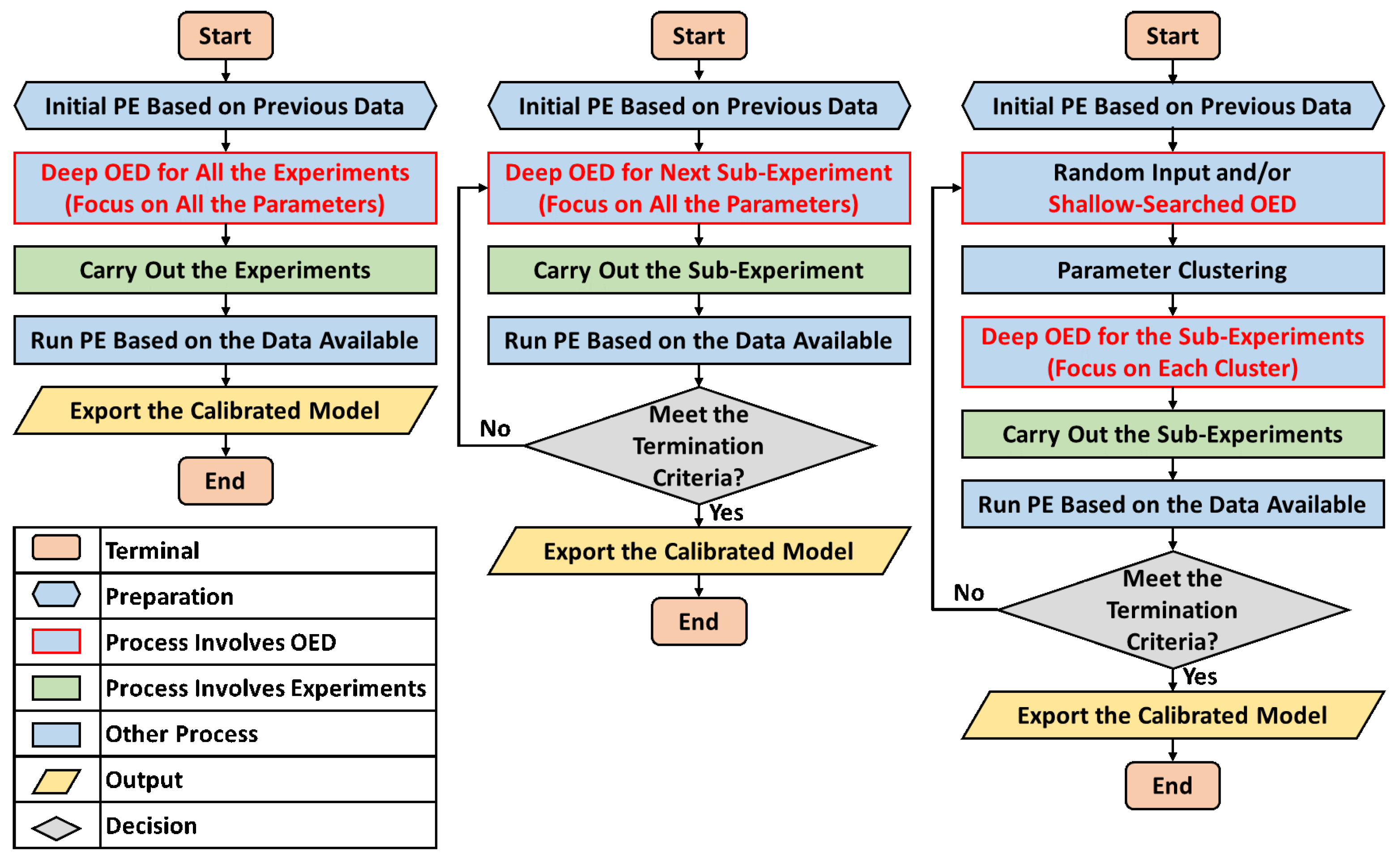
2.5. Details of the Experimental Design

The development in experimental techniques has significantly expanded the feasible experimental design space. For example, modern microfluidics allows high accuracy dynamic stimuli control and continuous observation of yeast cells [62,63]. To make the in-silico experiments (i.e. computer-based simulations) in this study close to wet-lab experiment situations, this paper considers an example of microfluidic-based experiments with a microfluidic chip designed by Ferry et al. [62]. The duration for each sub-experiment is set as 24 h (the time for cells to grow and fill up the cell chamber) with sampling frequency as 5 min (to limit the damage caused by photo-toxicity). In each experiment, cells are prepared at the steady-state with minimum expression level (in practice, it can be achieved by growing cells overnight without the IPTG inducer). During the experiment, the IPTG concentration varies seven times and forms eight steps with a 3-h-long duration for each step. The IPTG concentration at each step is selected from the range of 0.1∼100 $\mathsf{\mu }$M.

The in-silico experiments, parameter estimation (PE), and optimal experimental design (OED) procedures are carried out in MATLAB with AMIGO2 toolbox [50]. Following the previous study on this topic [3], the parameter estimation is carried out as the weighted least squares fitting, with the weight set to be the inverse of standard deviation of observation. As recommended by the AMIGO2 developer team [64,65], and to make the results comparable to previous study [3], the non-linear solver used for PE and OED is the enhanced scatter search (eSS, [66]) with the Nelder-Mead simplex algorithm (fminsearch function in MATLAB, [67]) as the hybrid local solver. It is worth mentioning that there are also other widely used metaheuristic solvers which may further improve the convergence, such as CMA-ES [68,69] and FST-PSO [70].

This study considers four experiment approaches: off-line OED, on-line OED, cluster-based OED, and experiments with randomised experimental design. Similar to the concepts defined in the previous study from Bandiera et al. [3], off-line and on-line OED are the two current OED approaches that optimise the accuracy of all the parameters in every sub-experiment. The difference is that off-line OED optimises the design of all the sub-experiments before carrying out any of them, while the on-line OED optimises one sub-experiment at a time, carry it out, and then updates the parameter estimation after every sub-experiment. Cluster-based OED runs the parameter clustering before OED, and then optimises the sub-experiment so that the accuracy of only one parameter cluster is focused in each. Random stimuli is the case that for all the sub-experiments, the input values at each step are randomly selected in the feasible range in logged scale. Figure 4 shows the flow charts of the OED approaches. Notice that the off-line and cluster-based OEDs are also suitable for parallel experiments, while the on-line OED cannot be carried out in this way.

It is noticeable in Figure 4 that there are shallow and deep searched OED. They refer to the searching of the optimal design with different maximum numbers of evaluations (500 for shallow and 50,000 for deep in this study). It is because deep-searched OEDs are used to find the exact optimal design, while the shallow-searched OED is just for generating reference data for parameter clustering as a supplement to the randomised stimuli. Moreover, another consideration is that biochemical systems (including the one considered in this study) usually contain non-linear parts [71,72,73], and it is broadly agreed that there is not yet an algorithm for general non-linear problems that could guarantee to find the globally optimal solution within a finite number of evaluations [74,75,76]. For the eSS method and most of the stochastic searching algorithms, a higher number of evaluations leads to a higher chance of finding the globally optimal solution [77,78]. In other words, shallow-searched OED also provides references to know “the accuracy for which parameters can be easily optimised at the same time”.

3. Results

3.1. Results of Parameter Clustering

3.1.1. Clustering Results with the Best Estimated Value Set

In this study, 30 in-silico trials with random stimuli and 30 trials with shallow-searched OED are generated as the references for clustering. As mentioned previously, there are two approaches for parameter clustering: sensitivity-based one and FIM-based one.

Although both the random stimuli and shallow-searched OED can provide evidences for clustering, it is necessary to check if the informativeness of these two samples sets are not significantly different. Considering both of these two groups of experiments could form a broader reference for clustering, but it may also mislead the clustering results if they are significantly different in the aspect of informativeness. It is because the point of parameter clustering is to find which of the parameters have the potential to be optimised for informativeness with a common stimulus pattern, not to searching for the informativeness difference between random stimuli and shallow-searched OED.

Figure 5 compares the observable mean squared sensitivity (defined as Equation (4)) in experiments with both random stimuli and shallow-search OED with the “true” parameter value set (the value set used for generating the in-silico experimental data). Moreover, Wilcoxon rank-sum tests (equivalent to Mann-Whitney U-tests) show that the shallow-searched OEDs lead to significantly higher medians of averaged sensitivities in both parameter cluster 1 ($p=3.16\times {10}^{-5}$) and cluster 2 ($p=8.50\times {10}^{-4}$).

In this case study, the shallow-searched OEDs lead to observations that are significantly more sensitivity to parameter value changes, compared to randomised stimuli. Therefore, only the OED data are used for parameter clustering (otherwise, the difference between random stimuli and OED may mislead the clustering). The results are shown in Figure 6.

It can be seen that in both sensitivity-based and FIM-based parameter clustering, the parameters corresponding to the only non-linear part, the Hill-function, is separated from the rest of parameters (refer to the model Equation (1), $V{m}_1$ can be considered as a scaling factor as a part of the ’linear part’ of this model). It is supported by the previous comparison between random stimuli and OEDs, which suggests that the parameters for linear and non-linear ’parts’ have different stimuli-informativeness patterns. The FIM-based clustering further separates the Michaelis-Menten coefficient $Km$ and the Hill coefficient $h_1$. It is understandable because $Km$ reflects the IPTG concentration that leads to a 50% promotion level, and $h_1$ reflects how sharp the promotion level changes with the IPTG concentration. So the most informative stimuli pattern for calibrating these two parameters are different. Overall, the clustering results of the two different approaches give slightly different results, but they both reflect the inner property of the model.

3.1.2. Clustering Results with Randomised Value Sets

In real model calibration cases, the initial parameter guess does not equal the “true” value set. To investigate how the clustering results are affected by the parameter values, the clustering is carried out with 30 trials with parameter values randomly chosen in the feasible space (in logged scale). Results show that the cluster numbers do change with the parameter values (Figure 7), and so as which parameters belong to which cluster (Figure 8). It is worth mentioning that the plot design for visualising the cluster results is particularly modified based on arc diagrams and chord diagrams. The orange nodes are added to show how common one element belongs to a cluster without any other elements, the node orders and the shapes of the arcs are also modified so that readers can more easily find the element combinations that are commonly appeared in one cluster.

The case corresponding to the best-fitting parameter sets (i.e., the previous Section 3.1.1) belongs to the top-left box. Most of the trials lead to two clusters in both sensitivity-based and FIM-based clustering.

Figure 8 shows that the sensitivity-based and FIM-based clustering share some common results and slightly different in the treatments of parameter ${\alpha }_1$ (the parameter decides the basial expression level of Citrine). 50% of the sensitivity-based and FIM-based clustering with randomised parameter guesses grouped $h_1$ as an individual cluster. According to the sensitivity-based clustering, ${\alpha }_1$ has a weak and not robust connection to the other parameters, whereas in the FIM-based clustering ${\alpha }_1$ shares a common cluster with the other ’linear part parameters’ in most of the cases. There is not an obvious explanation for this according to the knowledge of the author. One information which may be helpful is that different from the other parameters, ${\alpha }_1$ does not contribute to any expression change corresponding to the IPTG concentration.

In short conclusion, the clustering results vary with the initial parameter guesses but not completely random. The results still reflect the inner property of the model and connections between parameters.

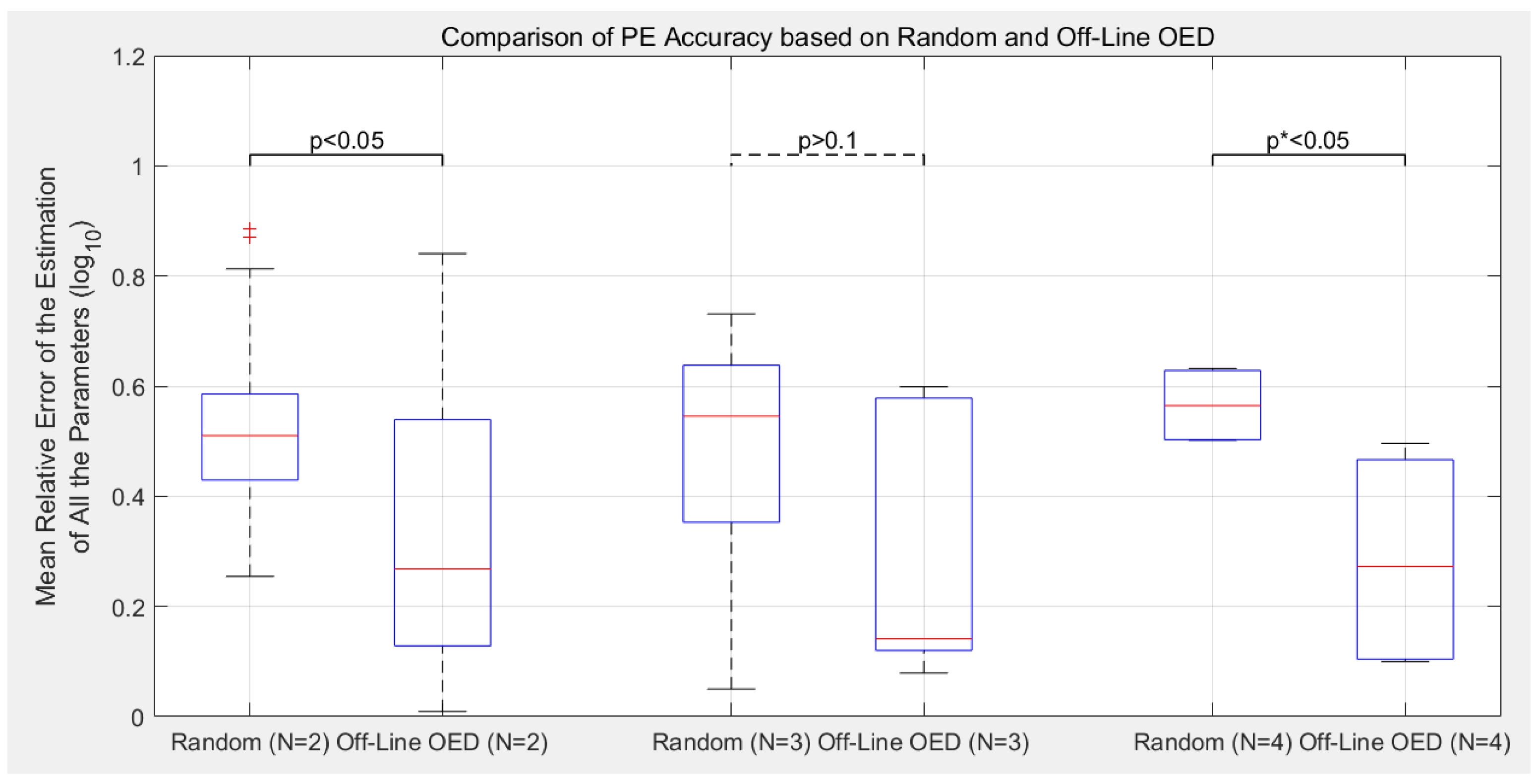
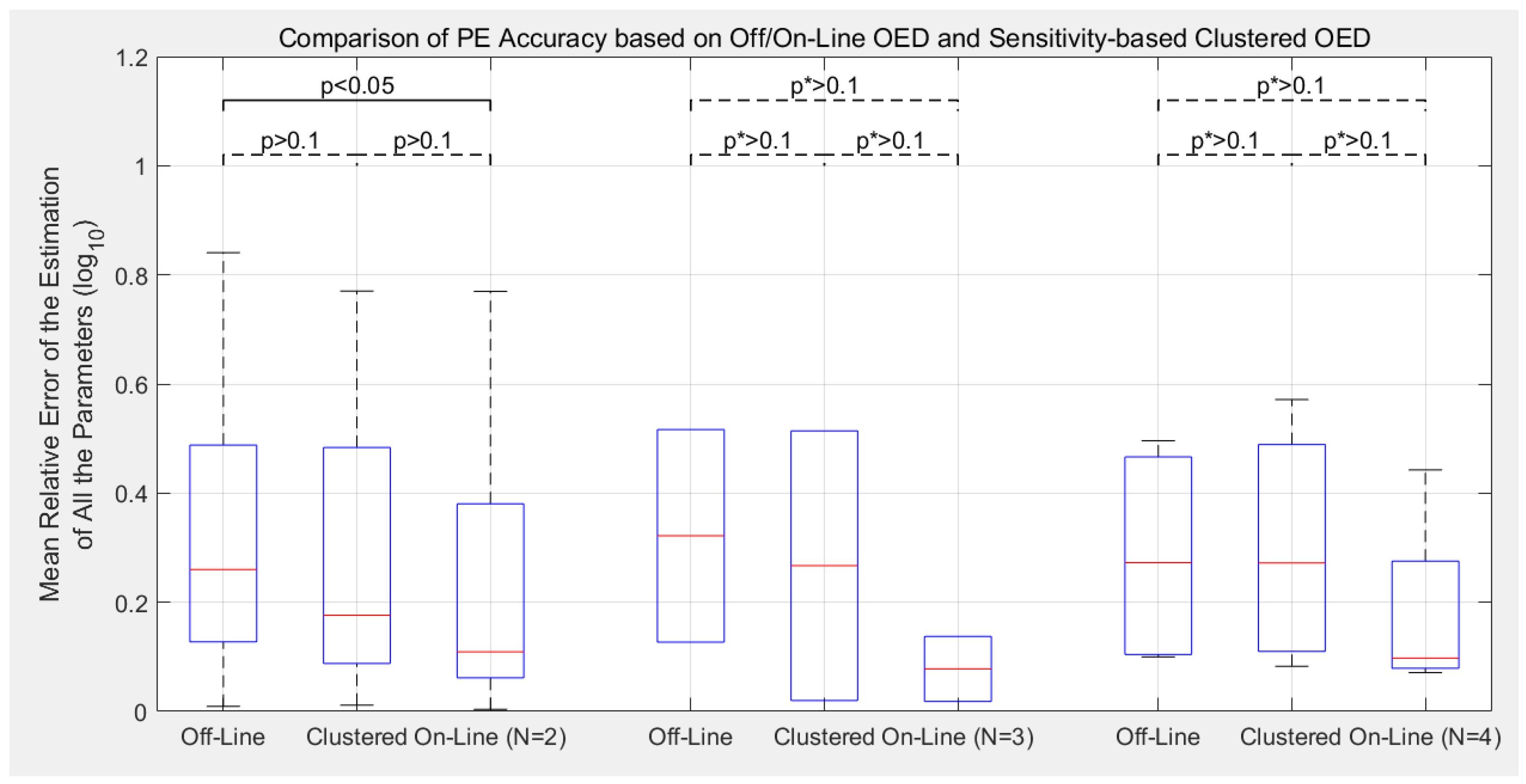
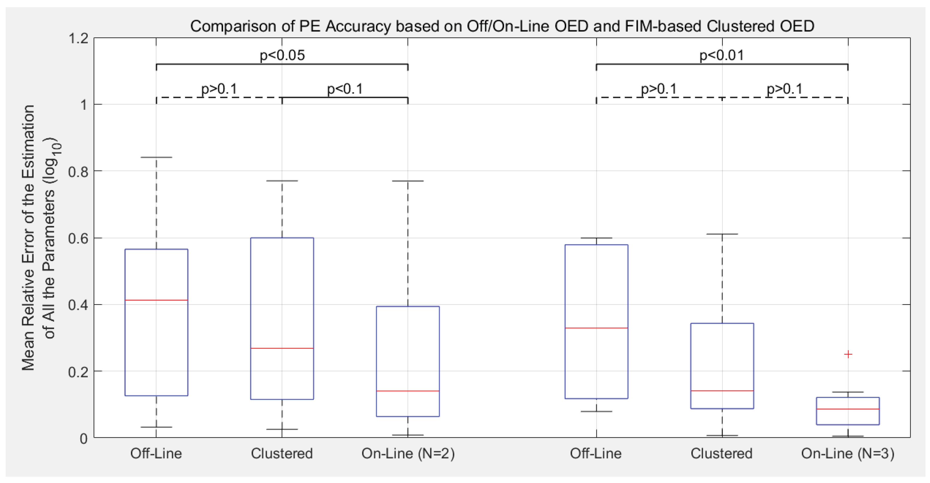
3.2. Estimation Accuracy with Different Experimental Designs

Figure 9, Figure 10 and Figure 11 show the comparison of the estimation accuracy. Notice that the data are grouped according to the number of clusters. It is because only experiment sequences with the same number of sub-experiments are comparable. It is not informative to compare and say that a parameter estimation based on more experimental data is expected to be more accurate. It is also because, as shown in Section 3.1.2, the numbers of clusters also depend on the initial estimations which affects the final estimation accuracy by itself.

Similar to the previous study from Bandiera et al. [3], the mean relative error is used to quantify the overall accuracy of parameter estimations. Its definition is given as Equation (8).

$${\epsilon }^j=\frac{1}{N_{\theta }}\sum _{i=1}^{N_{\theta }}\left|lo{g}_{10}\frac{{\theta }_i^j}{{\theta }_i^{*}}\right|$$

(8)

where j is the experiment index, i is the parameter index, $N_{\theta }$ is the number of parameters, ${\theta }_i^j$ is the fitted parameter value according to the experimental observations, and ${\theta }_i^{*}$ is the true parameter value which is used to generate the in-silico experimental data. If the estimations are exactly equal to the true parameter set, ${\epsilon }^j$ would equal to zero. Larger values represent less accurate estimations.

For all the trials, the in-silico experiments with random stimuli and off-line OED with a sub-experiment number correspond to the cluster number N are carried out for this comparison. Because the sensitivity-based and FIM-based cluster numbers could be different, the total number of experiments in this comparison is larger than 30 (42 trials to be precise). In cases, off-line OED leads statistically more accurate parameter estimations. The comparison for three sub-experiments (N = 3) does not show a significant result. However, both the median and average error from the off-line OED samples are lower than the ones with random stimuli. Among all the trials, off-line OEDs lead to 31.7% lower mean relative error in average compared to randomised stimuli.

In both Figure 10 and Figure 11, cluster-based OED approaches leads to estimations that are not statistically worse than off-line OED, with lower median error in most of the cases. Keep in mind that the complexity of solving the cluster-based OED is simpler than the traditional off-line and on-line OED approaches. Compare to the OED cases that focus on all the seven model parameters, the computational cost for FIM-based OED reduces by 49.0% ∼ 91.8% depending on the parameters in the cluster. Among all the trials, Sensitivity-based clustered OEDs lead to 45.1% lower mean relative error in average compared to randomised stimuli, and FIM-based clustered OEDs lead to 39.7% error reduction. Their performances are better than off-line OED (31.7%) but worse than on-line OED (57.2%).

4. Conclusions and Prospect

This study investigated two approaches to improve the efficiency of FIM-based OED by introducing parameter clustering analysis. The main conclusions from this work are:

• Compared to the previous off-line OED approach, the proposed cluster-based OED with either the sensitivity-based or FIM-based approaches could achieve equal or even slightly better calibration accuracy with at least 49.0% reduction in computational cost;
• Although the main purpose of introducing parameter clustering is for reducing the computational cost of OED, not for increasing the PE accuracy, cluster-based OEDs lead to lower estimation error in average in this benchmark. Sensitivity-based approach reduces the mean relative error of parameter estimation (defined as Equation (8)) by 19.6% in average, and the FIM-based approach reduces by 11.8%;
• Compare to the previously proposed on-line OED approach, the model calibration accuracy of cluster-based OED does not statistically out-compete the current approach in this benchmark test. Meanwhile, it is worth mentioning that cluster-based OED is suitable for parallel experiments, but on-line OED is not;
• Compared to previous applications of parameter clustering in the OED procedure, this study provides a completely different approach of using the clustering results. Instead of guiding the selection of fitting parameters, the proposed methods keep the initial selection of fitting parameters and aim at achieving more informative experimental designs;
• Both sensitivity-based and FIM-based clustering provide understandable parameter clustering results, which could provide a reference for understanding the model structure and simplifying the OED procedure.
• The proposed method for visualising the clustering results is of great potential to provide efficient graphical help to understand the model mechanisms and inner properties.

This study is just a start of implementing the cluster-based OED. It would be helpful to examine its efficiency with wet-lab experiments, and also to validate its benefits with representative PE solvers such as CMA-ES and FST-PSO. Another future work is to apply this method to larger and more complex models to exploit its potential in visualising the connects between parameters.

References

1. Gutenkunst, R.N.; Waterfall, J.J.; Casey, F.P.; Brown, K.S.; Myers, C.R.; Sethna, J.P. Universally sloppy parameter sensitivities in systems biology models. PLoS Comput. Biol. 2007, 3, e189. [Google Scholar] [CrossRef] [PubMed] [Green Version]
2. Bouvin, J.; Cajot, S.; D’Huys, P.J.; Ampofo-Asiama, J.; Anné, J.; Van Impe, J.; Geeraerd, A.; Bernaerts, K. Multi-objective experimental design for 13C-based metabolic flux analysis. Math. Biosci. 2015, 268, 22–30. [Google Scholar] [CrossRef] [PubMed]
3. Bandiera, L.; Hou, Z.; Kothamachu, V.B.; Balsa-Canto, E.; Swain, P.S.; Menolascina, F. On-line optimal input design increases the efficiency and accuracy of the modelling of an inducible synthetic promoter. Processes 2018, 6, 148. [Google Scholar] [CrossRef] [Green Version]
4. Nimmegeers, P.; Bhonsale, S.; Telen, D.; Van Impe, J. Optimal experiment design under parametric uncertainty: A comparison of a sensitivities based approach versus a polynomial chaos based stochastic approach. Chem. Eng. Sci. 2020, 221, 115651. [Google Scholar] [CrossRef]
5. Moles, C.G.; Mendes, P.; Banga, J.R. Parameter estimation in biochemical pathways: A comparison of global optimization methods. Genome Res. 2003, 13, 2467–2474. [Google Scholar] [CrossRef] [PubMed] [Green Version]
6. Rodriguez-Fernandez, M.; Mendes, P.; Banga, J.R. A hybrid approach for efficient and robust parameter estimation in biochemical pathways. Biosystems 2006, 83, 248–265. [Google Scholar] [CrossRef] [PubMed]
7. Franceschini, G.; Macchietto, S. Model-based design of experiments for parameter precision: State of the art. Chem. Eng. Sci. 2008, 63, 4846–4872. [Google Scholar] [CrossRef]
8. Rojas, C.R.; Welsh, J.S.; Goodwin, G.C.; Feuer, A. Robust optimal experiment design for system identification. Automatica 2007, 43, 993–1008. [Google Scholar] [CrossRef]
9. Telen, D.; Houska, B.; Logist, F.; Van Derlinden, E.; Diehl, M.; Van Impe, J. Optimal experiment design under process noise using Riccati differential equations. J. Process Control 2013, 23, 613–629. [Google Scholar] [CrossRef] [Green Version]
10. Bandara, S.; Schlöder, J.P.; Eils, R.; Bock, H.G.; Meyer, T. Optimal experimental design for parameter estimation of a cell signaling model. PLoS Comput. Biol. 2009, 5, e1000558. [Google Scholar] [CrossRef] [PubMed]
11. Kreutz, C.; Timmer, J. Systems biology: Experimental design. FEBS J. 2009, 276, 923–942. [Google Scholar] [CrossRef] [PubMed]
12. Komorowski, M.; Costa, M.J.; Rand, D.A.; Stumpf, M.P. Sensitivity, robustness, and identifiability in stochastic chemical kinetics models. Proc. Natl. Acad. Sci. USA 2011, 108, 8645–8650. [Google Scholar] [CrossRef] [PubMed] [Green Version]
13. Gorman, J.D.; Hero, A.O. Lower bounds for parametric estimation with constraints. IEEE Trans. Inf. Theory 1990, 36, 1285–1301. [Google Scholar] [CrossRef]
14. Stoica, P.; Ng, B.C. On the Cramér-Rao bound under parametric constraints. IEEE Signal Process. Lett. 1998, 5, 177–179. [Google Scholar] [CrossRef]
15. Baltes, M.; Schneider, R.; Sturm, C.; Reuss, M. Optimal experimental design for parameter estimation in unstructured growth models. Biotechnol. Prog. 1994, 10, 480–488. [Google Scholar] [CrossRef]
16. Lindner, P.F.O.; Hitzmann, B. Experimental design for optimal parameter estimation of an enzyme kinetic process based on the analysis of the Fisher information matrix. J. Theor. Biol. 2006, 238, 111–123. [Google Scholar] [CrossRef] [PubMed]
17. Chu, Y.; Hahn, J. Parameter set selection via clustering of parameters into pairwise indistinguishable groups of parameters. Ind. Eng. Chem. Res. 2009, 48, 6000–6009. [Google Scholar] [CrossRef]
18. Guedj, J.; Thiébaut, R.; Commenges, D. Practical identifiability of HIV dynamics models. Bull. Math. Biol. 2007, 69, 2493–2513. [Google Scholar] [CrossRef] [PubMed] [Green Version]
19. Riviere, M.K.; Ueckert, S.; Mentré, F. An MCMC method for the evaluation of the Fisher information matrix for non-linear mixed effect models. Biostatistics 2016, 17, 737–750. [Google Scholar] [CrossRef] [PubMed]
20. Nguyen, T.T.; Mentré, F. Evaluation of the Fisher information matrix in nonlinear mixed effect models using adaptive Gaussian quadrature. Comput. Stat. Data Anal. 2014, 80, 57–69. [Google Scholar] [CrossRef] [Green Version]
21. Telen, D.; Logist, F.; Van Derlinden, E.; Tack, I.; Van Impe, J. Optimal experiment design for dynamic bioprocesses: A multi-objective approach. Chem. Eng. Sci. 2012, 78, 82–97. [Google Scholar] [CrossRef]
22. Manesso, E.; Sridharan, S.; Gunawan, R. Multi-objective optimization of experiments using curvature and fisher information matrix. Processes 2017, 5, 63. [Google Scholar] [CrossRef] [Green Version]
23. Ueckert, S.; Mentré, F. A new method for evaluation of the Fisher information matrix for discrete mixed effect models using Monte Carlo sampling and adaptive Gaussian quadrature. Comput. Stat. Data Anal. 2017, 111, 203–219. [Google Scholar] [CrossRef] [Green Version]
24. Arora, S.; Barak, B. Computational Complexity: A Modern Approach; Cambridge University Press: Cambridge, UK, 2009. [Google Scholar]
25. Pronzato, L.; Walter, É. Robust experiment design via stochastic approximation. Math. Biosci. 1985, 75, 103–120. [Google Scholar] [CrossRef]
26. Machado, V.C.; Tapia, G.; Gabriel, D.; Lafuente, J.; Baeza, J.A. Systematic identifiability study based on the Fisher Information Matrix for reducing the number of parameters calibration of an activated sludge model. Environ. Model. Softw. 2009, 24, 1274–1284. [Google Scholar] [CrossRef]
27. Hassanein, W.; Kilany, N. DE-and EDP _{M}-compound optimality for the information and probability-based criteria. Hacet. J. Math. Stat. 2019, 48, 580–591. [Google Scholar]
28. Logist, F.; Telen, D.; Van Derlinden, E.; Van Impe, J.F. Multi-objective optimisation approach to optimal experiment design in dynamic bioprocesses using ACADO toolkit. In Computer Aided Chemical Engineering; Elsevier: Amsterdam, The Netherlands, 2011; Volume 29, pp. 462–466. [Google Scholar]
29. Balsa-Canto, E.; Alonso, A.A.; Banga, J.R. Computational procedures for optimal experimental design in biological systems. IET Syst. Biol. 2008, 2, 163–172. [Google Scholar] [CrossRef] [PubMed]
30. Kravaris, C.; Hahn, J.; Chu, Y. Advances and selected recent developments in state and parameter estimation. Comput. Chem. Eng. 2013, 51, 111–123. [Google Scholar] [CrossRef]
31. Dai, W.; Bansal, L.; Hahn, J. Parameter set selection for signal transduction pathway models including uncertainties. IFAC Proc. Vol. 2014, 47, 815–820. [Google Scholar] [CrossRef] [Green Version]
32. Gábor, A.; Villaverde, A.F.; Banga, J.R. Parameter identifiability analysis and visualization in large-scale kinetic models of biosystems. BMC Syst. Biol. 2017, 11, 1–16. [Google Scholar] [CrossRef] [PubMed] [Green Version]
33. Lee, D.; Jayaraman, A.; Kwon, J.S.I. Identification of a time-varying intracellular signalling model through data clustering and parameter selection: Application to NF-κ B signalling pathway induced by LPS in the presence of BFA. IET Syst. Biol. 2019, 13, 169–179. [Google Scholar] [CrossRef] [PubMed]
34. Nienałtowski, K.; Włodarczyk, M.; Lipniacki, T.; Komorowski, M. Clustering reveals limits of parameter identifiability in multi-parameter models of biochemical dynamics. BMC Syst. Biol. 2015, 9, 1–9. [Google Scholar] [CrossRef] [PubMed] [Green Version]
35. Walter, É.; Pronzato, L. Qualitative and quantitative experiment design for phenomenological models—A survey. Automatica 1990, 26, 195–213. [Google Scholar] [CrossRef]
36. Aster, R.C.; Borchers, B.; Thurber, C.H. Parameter Estimation and Inverse Problems; Elsevier: Amsterdam, The Netherlands, 2018. [Google Scholar]
37. Gnugge, R.; Dharmarajan, L.; Lang, M.; Stelling, J. An orthogonal permease–inducer–repressor feedback loop shows bistability. ACS Synth. Biol. 2016, 5, 1098–1107. [Google Scholar] [CrossRef] [PubMed]
38. Raue, A.; Schilling, M.; Bachmann, J.; Matteson, A.; Schelke, M.; Kaschek, D.; Hug, S.; Kreutz, C.; Harms, B.D.; Theis, F.J.; et al. Lessons learned from quantitative dynamical modeling in systems biology. PLoS ONE 2013, 8, e74335. [Google Scholar] [CrossRef]
39. Liepe, J.; Filippi, S.; Komorowski, M.; Stumpf, M.P. Maximizing the information content of experiments in systems biology. PLoS Comput. Biol. 2013, 9, e1002888. [Google Scholar] [CrossRef] [PubMed] [Green Version]
40. Vanlier, J.; Tiemann, C.; Hilbers, P.; Van Riel, N. Parameter uncertainty in biochemical models described by ordinary differential equations. Math. Biosci. 2013, 246, 305–314. [Google Scholar] [CrossRef] [PubMed]
41. Raue, A.; Steiert, B.; Schelker, M.; Kreutz, C.; Maiwald, T.; Hass, H.; Vanlier, J.; Tönsing, C.; Adlung, L.; Engesser, R.; et al. Data2Dynamics: A modeling environment tailored to parameter estimation in dynamical systems. Bioinformatics 2015, 31, 3558–3560. [Google Scholar] [CrossRef] [PubMed] [Green Version]
42. Chen, M.; Li, F.; Wang, S.; Cao, Y. Stochastic modeling and simulation of reaction-diffusion system with Hill function dynamics. BMC Syst. Biol. 2017, 11, 1–11. [Google Scholar] [CrossRef] [PubMed] [Green Version]
43. Wachtel, A.; Rao, R.; Esposito, M. Thermodynamically consistent coarse graining of biocatalysts beyond Michaelis–Menten. New J. Phys. 2018, 20, 042002. [Google Scholar] [CrossRef]
44. Gilchrist, M.A.; Wagner, A. A model of protein translation including codon bias, nonsense errors, and ribosome recycling. J. Theor. Biol. 2006, 239, 417–434. [Google Scholar] [CrossRef] [PubMed]
45. Pelechano, V.; Chávez, S.; Pérez-Ortín, J.E. A complete set of nascent transcription rates for yeast genes. PLoS ONE 2010, 5, e15442. [Google Scholar] [CrossRef] [PubMed]
46. Wang, Y.; Liu, C.L.; Storey, J.D.; Tibshirani, R.J.; Herschlag, D.; Brown, P.O. Precision and functional specificity in mRNA decay. Proc. Natl. Acad. Sci. USA 2002, 99, 5860–5865. [Google Scholar] [CrossRef] [PubMed] [Green Version]
47. Belle, A.; Tanay, A.; Bitincka, L.; Shamir, R.; O’Shea, E.K. Quantification of protein half-lives in the budding yeast proteome. Proc. Natl. Acad. Sci. USA 2006, 103, 13004–13009. [Google Scholar] [CrossRef] [PubMed] [Green Version]
48. Gordon, A.; Colman-Lerner, A.; Chin, T.E.; Benjamin, K.R.; Richard, C.Y.; Brent, R. Single-cell quantification of molecules and rates using open-source microscope-based cytometry. Nat. Methods 2007, 4, 175–181. [Google Scholar] [CrossRef] [PubMed]
49. Fisher, R.A. Design of experiments. Br. Med. J. 1936, 1, 554. [Google Scholar] [CrossRef]
50. Balsa-Canto, E.; Henriques, D.; Gábor, A.; Banga, J.R. AMIGO2, a toolbox for dynamic modeling, optimization and control in systems biology. Bioinformatics 2016, 32, 3357–3359. [Google Scholar] [CrossRef] [PubMed] [Green Version]
51. Salton, G.; Buckley, C. Term-weighting approaches in automatic text retrieval. Inf. Process. Manag. 1988, 24, 513–523. [Google Scholar] [CrossRef] [Green Version]
52. Jang, J.; Smyth, A.W. Model updating of a full-scale FE model with nonlinear constraint equations and sensitivity-based cluster analysis for updating parameters. Mech. Syst. Signal Process. 2017, 83, 337–355. [Google Scholar] [CrossRef]
53. Shahverdi, H.; Mares, C.; Wang, W.; Mottershead, J. Clustering of parameter sensitivities: Examples from a helicopter airframe model updating exercise. Shock Vib. 2009, 16, 75–87. [Google Scholar] [CrossRef]
54. Everitt, B.S.; Landau, S.; Leese, M.; Stahl, D. Hierarchical clustering. In Cluster Analysis; Wiley: Chichester, UK, 2011; Volume 5, pp. 71–110. [Google Scholar]
55. Hartigan, J.A. A K-means clustering algorithm: Algorithm AS 136. Appl. Stat. 1979, 28, 126–130. [Google Scholar] [CrossRef]
56. Arthur, D.; Vassilvitskii, S. k-Means++: The Advantages of Careful Seeding; Technical Report; Stanford University: Stanford, CA, USA, 2006. [Google Scholar]
57. Tibshirani, R.; Walther, G.; Hastie, T. Estimating the number of clusters in a data set via the gap statistic. J. R. Stat. Soc. Ser. B Stat. Methodol. 2001, 63, 411–423. [Google Scholar] [CrossRef]
58. Kaufman, L.; Rousseeuw, P.J. Finding Groups in Data: An Introduction to Cluster Analysis; John Wiley & Sons: Hoboken, NJ, USA, 2009; Volume 344. [Google Scholar]
59. Lallement, G.; Piranda, J. Localization methods for parametric updating of finite elements models in elastodynamics. In Proceedings of the 8th International Modal Analysis Conference, Kissimmee, FL, USA, 29 January–1 February 1990; pp. 579–585. [Google Scholar]
60. Caliński, T.; Harabasz, J. A dendrite method for cluster analysis. Commun. Stat. Theory Methods 1974, 3, 1–27. [Google Scholar] [CrossRef]
61. Davies, D.L.; Bouldin, D.W. A cluster separation measure. IEEE Trans. Pattern Anal. Mach. Intell. 1979, PAMI-1, 224–227. [Google Scholar] [CrossRef]
62. Ferry, M.S.; Razinkov, I.A.; Hasty, J. Microfluidics for synthetic biology: From design to execution. Methods Enzymol. 2011, 497, 295–372. [Google Scholar] [PubMed] [Green Version]
63. Scheler, O.; Postek, W.; Garstecki, P. Recent developments of microfluidics as a tool for biotechnology and microbiology. Curr. Opin. Biotechnol. 2019, 55, 60–67. [Google Scholar] [CrossRef] [PubMed]
64. Balsa-Canto, E.; Bandiera, L.; Menolascina, F. Optimal Experimental Design for Systems and Synthetic Biology Using AMIGO2. In Synthetic Gene Circuits; Springer: Berlin/Heidelberg, Germany, 2021; pp. 221–239. [Google Scholar]
65. Villaverde, A.F.; Fröhlich, F.; Weindl, D.; Hasenauer, J.; Banga, J.R. Benchmarking optimization methods for parameter estimation in large kinetic models. Bioinformatics 2019, 35, 830–838. [Google Scholar] [CrossRef] [PubMed]
66. Egea, J.A.; Martí, R.; Banga, J.R. An evolutionary method for complex-process optimization. Comput. Oper. Res. 2010, 37, 315–324. [Google Scholar] [CrossRef]
67. Lagarias, J.C.; Reeds, J.A.; Wright, M.H.; Wright, P.E. Convergence properties of the Nelder–Mead simplex method in low dimensions. SIAM J. Optim. 1998, 9, 112–147. [Google Scholar] [CrossRef] [Green Version]
68. Hansen, N.; Müller, S.D.; Koumoutsakos, P. Reducing the time complexity of the derandomized evolution strategy with covariance matrix adaptation (CMA-ES). Evol. Comput. 2003, 11, 1–18. [Google Scholar] [CrossRef] [PubMed]
69. Hansen, N. The CMA evolution strategy: A comparing review. In Towards a New Evolutionary Computation; Springer: Heidelberg/Berlin, Germany, 2006; pp. 75–102. [Google Scholar]
70. Nobile, M.S.; Cazzaniga, P.; Besozzi, D.; Colombo, R.; Mauri, G.; Pasi, G. Fuzzy Self-Tuning PSO: A settings-free algorithm for global optimization. Swarm Evol. Comput. 2018, 39, 70–85. [Google Scholar] [CrossRef]
71. Bashor, C.J.; Patel, N.; Choubey, S.; Beyzavi, A.; Kondev, J.; Collins, J.J.; Khalil, A.S. Complex signal processing in synthetic gene circuits using cooperative regulatory assemblies. Science 2019, 364, 593–597. [Google Scholar] [CrossRef] [PubMed]
72. Bashor, C.J.; Horwitz, A.A.; Peisajovich, S.G.; Lim, W.A. Rewiring cells: Synthetic biology as a tool to interrogate the organizational principles of living systems. Annu. Rev. Biophys. 2010, 39, 515–537. [Google Scholar] [CrossRef] [PubMed] [Green Version]
73. Ferrell, J.E., Jr.; Xiong, W. Bistability in cell signaling: How to make continuous processes discontinuous, and reversible processes irreversible. Chaos Interdiscip. J. Nonlinear Sci. 2001, 11, 227–236. [Google Scholar] [CrossRef] [PubMed]
74. Babu, B.; Angira, R. Modified differential evolution (MDE) for optimization of non-linear chemical processes. Comput. Chem. Eng. 2006, 30, 989–1002. [Google Scholar] [CrossRef]
75. Onwubolu, G.C.; Babu, B. New Optimization Techniques in Engineering; Springer: Berlin/Heidelberg, Germany, 2013; Volume 141. [Google Scholar]
76. Avriel, M. Nonlinear Programming: Analysis and Methods; Courier Corporation: North Chelmsford, MA, USA, 2003. [Google Scholar]
77. Gong, W.; Cai, Z.; Ling, C.X.; Li, H. Enhanced differential evolution with adaptive strategies for numerical optimization. IEEE Trans. Syst. Man Cybern. Part B 2010, 41, 397–413. [Google Scholar] [CrossRef] [PubMed]
78. Gong, W.; Fialho, A.; Cai, Z.; Li, H. Adaptive strategy selection in differential evolution for numerical optimization: An empirical study. Inf. Sci. 2011, 181, 5364–5386. [Google Scholar] [CrossRef]
Figure 1. The inducible promoter designed by Gnügge et al. [37]. (Figure is modified from a related work from Bandiera et al. [3]).
Processes 09 01053 g001
Figure 2. Illustration of the reactions considered in the model and how the parameters describes the reactions.
Processes 09 01053 g002
Figure 3. The “Full” FIM (left) can easily generate the FIMs for fitting subsets of parameters (right).
Processes 09 01053 g003
Figure 4. Flow charts of the off-line OED (left), on-line OED (middle), and cluster-based OED (right).
Processes 09 01053 g004
Figure 5. Comparing the observable mean squared sensitivity in experiments with both random stimuli and shallow-search OED. The significance levels come from one-sided Mann-Whitney U-tests because the distribution for random-stimuli experiments do not pass the Kolmogorov-Smirnov normality test.
Processes 09 01053 g005
Figure 6. Results of the Sensitivity-based and FIM-based parameter clustering. Parameter clusters can be distinguished by colours and superscripts.
Processes 09 01053 g006
Figure 7. Cluster numbers of randomised initial guesses.
Processes 09 01053 g007
Figure 8. Visualisation of the clustering results with randomised parameter value sets.
Processes 09 01053 g008
Figure 9. Comparison of the PE accuracy based on random and off-line OED experiments. p values stand for one-way t-test results (normal distributions), p* value is for one-sided Mann-Whitney U-tests. The random and off-line cases for N = 3 do not pass Kolmogorov-Smirnov normality test.
Processes 09 01053 g009
Figure 10. Comparison of the PE accuracy with off/on-line OED and sensitivity-base-clustered OED. p values stand for one-way t-test results (normal distributions), p* value is for one-sided Mann-Whitney U-tests.
Processes 09 01053 g010
Figure 11. Comparison of the PE accuracy with off/on-line OED and FIM-base-clustered OED. p values stand for one-way t-test results. All the distributions pass the Kolmogorov-Smirnov normality test.
Processes 09 01053 g011
Publisher’s Note: MDPI stays neutral with regard to jurisdictional claims in published maps and institutional affiliations.