1. Introduction
Economic efficiency and process safety are the most important factors in process industry. With the wide application of a distributed control system (DCS), a huge amount of process data can be collected and accumulated, which provides a great possibility for data-driven process monitoring [
1]. In recent years, a significant number of advanced monitoring methods have been proposed for early fault detection and diagnosis.
In DCS, each measurement is preset an operating range. An alarm will be triggered if any variable exceeds the predefined operating limit. However, unnecessary alarms can be quite overwhelming if there is no effective fault detection and diagnosis system [
2], which requires massive process knowledge and operation experience. To avoid this problem, many data-driven fault diagnosis methods are further proposed based on data collected from DCS. Among these methods, multivariate projection methods are the most commonly used by extracting key features of given process data and calculating the variable contribution with respect to the occurring fault [
3]. The contribution of each variable is plotted in a histogram for comparative analysis, and the variable with the highest contribution is considered as the root cause of the fault [
4]. The contribution plots are easy to calculate, but, for modern industrial chemical processes, variables interact with each other under the influence of equipment, stream loop, and control strategy. Once a fault occurs, the fast propagation of the contribution from root variable to other variables could be difficult to recognize [
5]. For this purpose, a causal reasoning model has been established and further combined with the contribution plots to solve this problem. If causal reasoning among variables could be obtained, the variables that have significant contributions could be arranged in a network diagram, from which the fault propagation could be obtained and then the real root cause could be located.
There are two ways to extract the causal logic among process variables, i.e., by knowledge and by data. For knowledge-based methods, intensive process knowledge and operational experience are required [
6]. With the increasing scale and complexity of chemical equipment and process topology, enough process knowledge is difficult to obtain and hard to update with an ever-changing operating condition, equipment aging and switch of control strategies. Motivated by this consideration, data driven methods are preferred with no prior process knowledge required.
Causal logic among process variables can also be described as correlation with a proper time lag between each pair of variables. One of the simplest and widely used methods is a Pearson correlation coefficient, but it is a linear correlation analysis, cannot be applied to extract nonlinear correlation, and also no time lag is considered. Several data driven causal reasoning methods like Granger causality [
7] and transfer entropy [
8] have been applied to build causal networks of process variables for root cause analysis. The Granger causality was first proposed as an economics theory to identify causal interactions and played an important role in explaining economic phenomena, which makes it more and more popular and can be applied to physics [
9], bioinformatics [
10], neuroscience [
11], and many other research fields. However, the Granger causality is established on partial least squares, which is a linear regression method too. For most systems in chemical industrial processes, the correlation among process variables is highly nonlinear. The application of Granger causality in these nonlinear systems is inadequate [
12]. To extract nonlinear correlation, transfer entropy is proposed based on information theory by calculating how much the uncertainty of one signal can be reduced if another signal is known [
13]. Transfer entropy is derived from information entropy (IE). Its mathematical calculation is established by estimating probability distribution; therefore, the nonlinear correlation between variables is well considered [
14]. It has been applied to determine the correlation among process variables in many nonlinear systems and shows a good performance on root cause analysis on faults defined in the Tennessee Eastman process (TEP) [
15].
Up to date, most causal reasoning methods are established based on data from normal operation conditions, which are then applied to illustrate a fault propagation path by a signed directed graph, once a fault is detected by a contribution plot. Due to a complex process topology of a chemical process, there are massive control loops to ensure stable operation of the system. When a fault occurs, the causal logic among process variables may change with the response of the control strategies, making the diagnosis results inconsistent with practical situations [
16]. In this work, the causal logic among process variables is obtained by analyzing mutual information (MI) from both historical data and real-time data, and then applied to identify fault propagation path and root cause. Better results are obtained compared with process knowledge-based methods and traditional data driven methods.
The following parts of this paper are arranged as follows: in
Section 2, the IE and MI are briefly introduced. The establishment of the digraph model based on time delayed mutual information (TDMI) is also detailed. In
Section 3, the procedure of the proposed fault diagnosis method and the selection of parameters are described, followed by a simple nonlinear simulation example. In
Section 4, the proposed method is applied to two industrial processes, TEP, and an industrial reforming process. The fault isolation results are shown and discussed. In
Section 5, the paper is concluded.
The abbreviations used in this work are summarized and interpreted as follows: MI represents mutual information; TDMI represents time delayed mutual information; DCS represents a distributed control system; IE represents information entropy; and TEP represents the Tennessee Eastman process.
2. Preliminaries
In this section, the IE, MI, kernel density estimation method, and digraph model are introduced as the basis of the proposed method.
2.1. Information Entropy
IE is proposed by Shannon based on the concept of thermodynamics entropy, representing the uncertainty of the variable [
17]. Given a random signal
X (
x1,
x2, …,
xn), its IE can be calculated as follows:
where
p(
xi) is the probability distribution of the sample
xi, with assumption that the IE is only related to the probability distribution of the variable. The probability distribution of the variable when its IE reaches the maximum value can be obtained by the Lagrange multiplier method:
where
λ is the Lagrange multiplier; in order to get the maximum value, the derivative in Equation (3) should be equal to 0. Then, the probability distribution
p(
x) can be solved as follows:
It can be concluded that the more uniform the probability distribution of the variable is, the less information the data contains, which means that the uncertainty of the variable is high. In contrast, if p(xi) = 1, variable x is completely determined, the IE value will be reduced to 0 according to Equation (1). In information theory, IE is extended to multi-variables to measure the uncertainty of a system.
2.2. Mutual Information
MI is a measurement for the correlation between two measurements from the aspect of IE. Given two random variables
x and
y, MI measures the effect on the uncertainty of
x if
y is given [
18]:
where
p(
x,
y) is joint probability distribution. According to Equation (7), if
x and
y are independent,
p(
x,
y) is equal to 0, and the MI will be 0, while, if there is a strong correlation between
x and
y, the MI will be large.
It can be known from the definition that the correlation measured by MI is only related to the probability distribution of the variables. Therefore, the quantification of MI is not limited to linear correlation between variables. Compared with commonly used Pearson correlation, MI is obtained based on both linear and nonlinear relationships between measurements. Take the following relationship as an example:
As shown in Equation (8), there is a trigonometric relationship between the variables x and y. The Pearson correlation coefficient between x and y is 0.0009032, which means there is almost no linear correlation between them, while the normalized MI is 0.4606, indicating that there is a certain correlation between the variables x and y.
Because of the symmetry in the calculation of MI, it can only reflect the degree of correlation between variables, but the chronological order of information between variable deviations is not available. To overcome this limitation, a time lag parameter can be introduced in the calculation to identify chronological order between variable deviations [
19]. The MI with a time lag can be defined as follows:
where
p(
x,
y +
τ) is the joint probability distribution of
X =
xt,
Y =
yt+τ, and
τ is the time lag parameter. The parameter
τ is determined when the MI reaches its peak. A positive
τ indicates that
x has a maximum correlation with future
y, which means that
x changes before
y, while negative
τ indicates that
x changes after
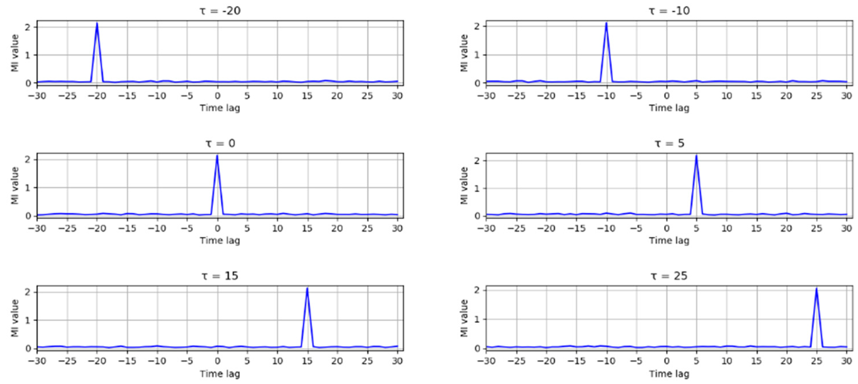
y. A simple nonlinear example is used to demonstrate this point:
where
x(
t) is a random variable follows a uniform distribution between 0 and 1, and
s1 is a random noise that follows a normal distribution with mean 0 and variance 0.02. Another variable
y(
t) has a nonlinear relationship with
x(
t −
τ), and
τ is set to several different values (−20, −10, 0, 5, 15, 25) to test the performance of TDMI. The MI of
x and
y with a time lag between −30 and 30 is shown in
Figure 1, and it can be seen that the MI reaches its peak when the time lag equals to the preset
τ in all the six situations. Due to the causal feature of industrial process, only variables changing earlier can possibly be the cause for other variables changing later; therefore, the TDMI can be applied to detect and analyze the causal relationship in nonlinear systems.
2.3. Kernel Density Estimation Method
Because the actual probability distribution of industrial data is unknown, the calculation of IE and MI mainly lies in the estimation of probability distribution. In this work, non-parametric probability density estimation methods are used, as it can be applied to estimate any form of probability distribution without assumptions. Among the commonly used non-parametric estimation methods, the kernel density estimation method is selected for its good performance on probability density estimation of a small number of samples [
20].
In the kernel density estimation method, a kernel function
K is applied to obtain a probability density function at every sample point, and all of these probability density functions are summed and averaged to obtain the estimate
p(
x):
where
n is the number of samples and
d is the window width which is adjusted with
n and the standard deviation of the variable
x to give a good estimation of the actual probability density function. Generally, a Gaussian function is used as the kernel function, and the optimal width is:
where
σ is the standard deviation of the variable. Equation (12) is derived by minimizing the mean integrated squared error function [
21].
2.4. Digraph Model
The identification of a cause and effect relationship in a system plays an important role in root cause diagnosis. The digraph model is a widely used intuitive tool to display the causal relationship. Generally, a digraph model can be described as G (N, A), where N is the nodes of the variables, and A is the directed arcs which connects cause nodes to consequent nodes.
A signed directed graph model is the most commonly used digraph model for fault diagnosis, in which a sign either positive or negative is set in each arc to represent whether the cause and consequent node change in the same direction or an opposite direction [
22]. Arcs and signs are usually established from process knowledge or expert experience of a process. Once a fault occurs, a sign in each node is set by comparing its value with a normal range determined previously. If the node value is higher than the normal range, the sign is set to positive. If the node value is lower than the normal range, the sign is set to negative. The sign is set to 0 if the node value is within the normal range. The sign of an arc in a consistent path is defined as positive, if the signs in both nodes are same, which means the nodes at both end of the arc changes in the same direction. Otherwise, the sign of the arc is defined as negative, if the signs in both nodes are opposite. Therefore, the fault propagation can be obtained by finding the consistent path in a signed directed graph model.
However, the challenge of the signed directed graph model is that it is hard to include enough process knowledge required in a complex industrial process. In this work, the digraph model is established by a data driven method. The nodes in the proposed model are obtained by finding the variable nodes whose IE is out of the normal range defined by previously calculated IE. The direction of the arcs is determined from the TDMI between two nodes. With the signed directed graph, the propagation path can be obtained only from process data, which provide a more objective information for fault diagnosis.
3. Fault Diagnosis Method with Information Solely Extracted from Process Data
In this section, IE and TDMI introduced in a previous section are used to propose a strategy for root cause diagnosis with both historical data and real-time data. The entire process of the proposed method and the details of the diagnosis strategy is described below.
3.1. Procedures for Process Fault Diagnosis
The basic idea of proposed diagnosis method is to estimate the probability density of process variables and then calculate their MI with different time lags. Generally, MI between variables, which are affected by faulty deviation, shows different characteristics from that under normal operating conditions. It can reach its maximum with a proper time lag, and the time dependency between these variables is therefore determined, which is usually depicted by a directed graph for fault propagation analysis.
As mentioned before, it requires significant computation to calculate the MI between every pair of variables if kernel density estimation is employed, as only part of the process variables will be affected under a faulty condition. These variables can be selected by their information entropies first. IE can be considered as the uncertainty or the amount of information contained in a variable. Given a random variable x in the industrial process, x generally fluctuates around its set point under the influence of noise under normal operation conditions. In this case, less information corresponds to a higher IE. Once a fault occurs in this process, the value of x will deviate from its set point, if it is affected. The amount of information contained in x will increase accordingly; in the meantime, its IE will decrease. On the other hand, the distribution of x will change under a faulty condition, and further affect its IE, which is only determined by its probability distribution according to its definition. Therefore, the variable is selected if its IE is out of the range obtained under normal operation conditions.
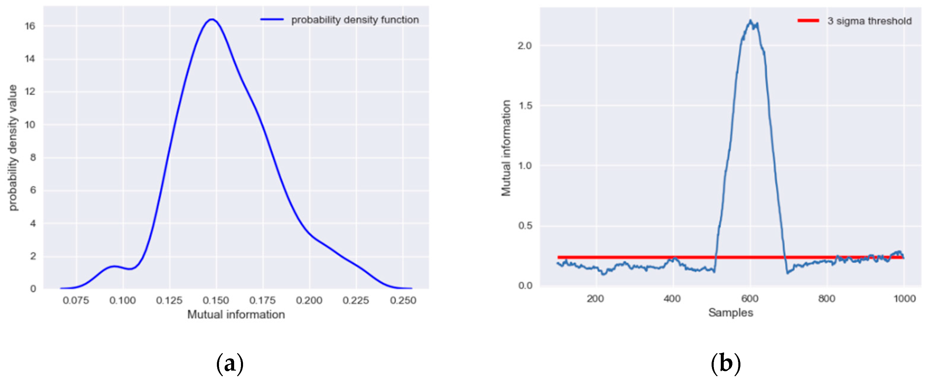
Once affected variables are identified, the time dependency between these variables can be determined by TDMI. Because there is no upper bound in MI, it is difficult to determine whether the variable correlation is significant based on MI values alone. When a fault occurs, MI shows different characteristics from that under normal operation conditions. When a system is under normal conditions, most process variables fluctuate randomly near their set value, and therefore the actual correlation between variables cannot be revealed. In this case, most MI is contributed by random noises. Once a fault occurs, corresponding changes will happen in certain variables. If there is causal relationship between these variables, the MI between them will increase with fault propagation and exceed the range determined under normal operation conditions. Next, a simple nonlinear example is applied to prove this point:
where
x,
y is random variables with a nonlinear correlation,
e1,
e2 is random noises that follows a normal distribution with variance 0.01 and 0.02. A set of 1000 samples is simulated and a ramp fault with a slope of 0.005 is introduced in
x from 500 to 600 samples. The MI of
x and
y is calculated with a moving window and compared under different conditions to prove the correlation between
x and
y. The distribution of MI under normal operation conditions is shown in
Figure 2a.
It can be seen that the MI follows a normal distribution with a relatively small mean. A three-sigma threshold is chosen here to define the significance level:
where
s(
x,
y) represents that the correlation between
x and
y is significant,
I(
x,
y) is the MI, and
μ and
σ are mean and standard deviation of MI calculated under normal operation conditions.
The MI of
x and
y from all the moving windows is shown in
Figure 2b. After the 500th sample, abnormal data are contained in the calculation windows of MI; therefore, the MI of
x and
y increases significantly and exceeds the threshold determined under normal conditions, indicating that there is a significant correlation between
x and
y.
3.2. The Implementation of the Proposed Fault Diagnosis Framework
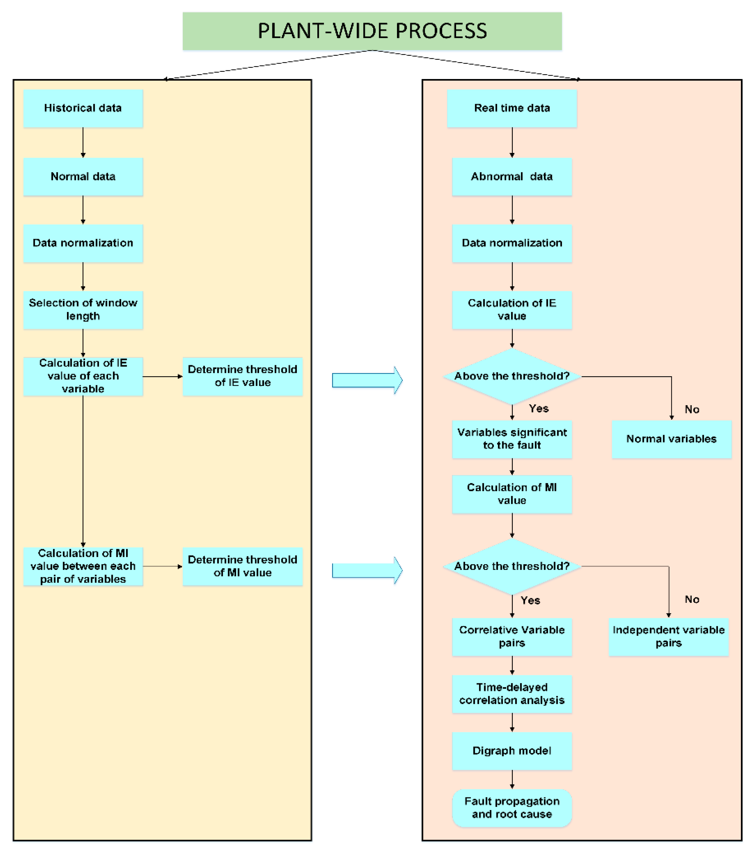
The flowchart of the proposed fault diagnosis method is shown in
Figure 3, and its implementation includes following two parts:
Offline parameters selection:
- (1)
Select data under normal operation conditions from historical data.
- (2)
Normalize the data and choose a suitable window length for the calculation of IE and MI.
- (3)
Calculate IE with a moving window based on kernel density estimation and determine the threshold of each variable.
- (4)
Calculate the MI of each pair of variables with the moving window and determine the threshold.
Online fault diagnosis:
- (1)
Collect real time data, once a fault is detected. These data are usually referred to as abnormal data.
- (2)
Calculate the IE of each variables using abnormal data and compare it with the thresholds determined previously. Variables that exceed the threshold are selected as the fault nodes in the directed digraph.
- (3)
Calculate MI of each pair of variables selected in the last step and compare it with the thresholds obtained offline. Variables that exceed the threshold indicate a significant correlation between them, and the nodes are connected with directed arcs in the digraph.
- (4)
Calculate the TDMI between correlated variables obtained in the last step to determine the direction of arcs.
- (5)
Isolate fault and analyze fault propagation path in the digraph. Root node can be regarded as the source of the fault, and child nodes are regarded as the consequent caused by the fault.
3.3. A Root Cause Identification in a Simulated Example
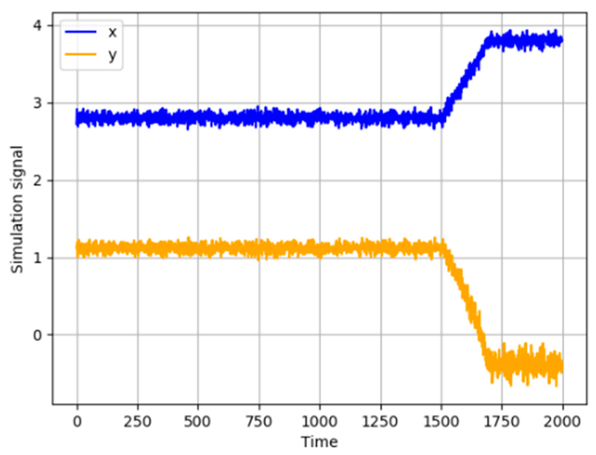
A nonlinear process contains two variables defined in following equations:
where
xt is a constant random variable with a random noise
e1 that follows a normal distribution with variance 0.01,
yt is another random variable that is caused by
xt. Time lag of the correlation between
xt and
yt is set to 3.
e2 is a random noise that follows a normal distribution with variance 0.02. A set of 2000 samples is simulated, and a ramp fault with the slope of 0.005 is introduced to
xt from the 1500th to 1700th sample. The variables are illustrated in
Figure 4. The first 1000 samples are selected as normal data to determine thresholds of IE and MI.
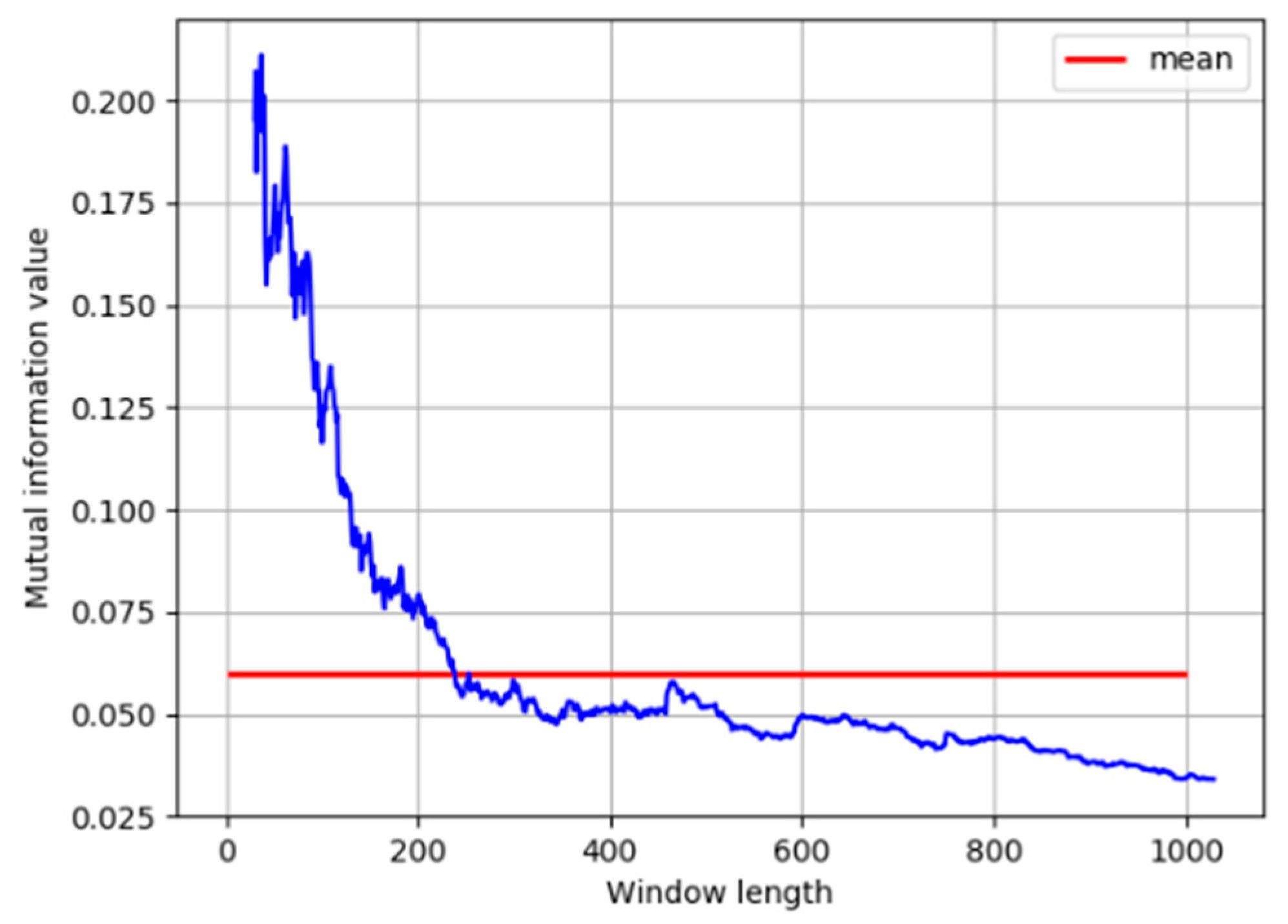
As discussed in the previous section, distribution characteristics of correlation between process variables are obtained by calculating MI with a moving window. The length of the moving window has a great influence on the estimation of probability density and further affects the calculation results of MI. For this concern, different window sizes need to be investigated. The MI calculated at window length from 30 to 1000 is shown in
Figure 5.
It can be seen that, when the window is short, the MI results are unreliable due to the insufficient number of samples in kernel density estimation. When the window reaches a certain size, the MI remains stable as the window length increases, and is close to its average value under all window sizes. Therefore, the window size is selected as 240.
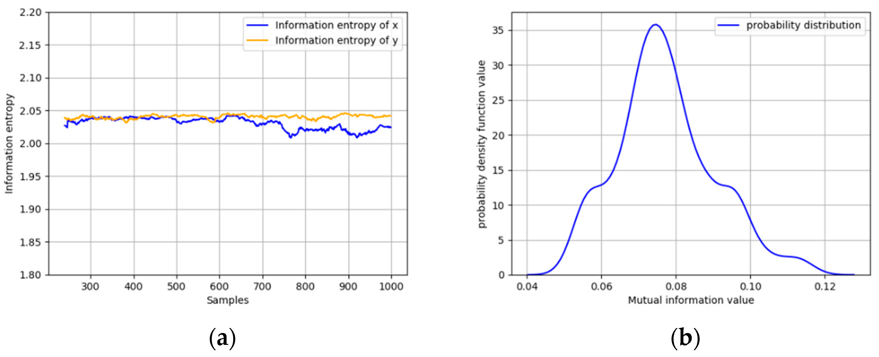
Then, thresholds of IE and MI are determined with the first 1000 normal data. The IE of
x and
y under normal operating conditions and the distribution of MI of
x and
y are shown in
Figure 6a,b. It can be obtained that the MI follows a normal distribution with mean 0.07728 and standard deviation 0.01315. As discussed before, a three-sigma threshold is selected as 0.15617, and the thresholds of IE are selected in the same way.
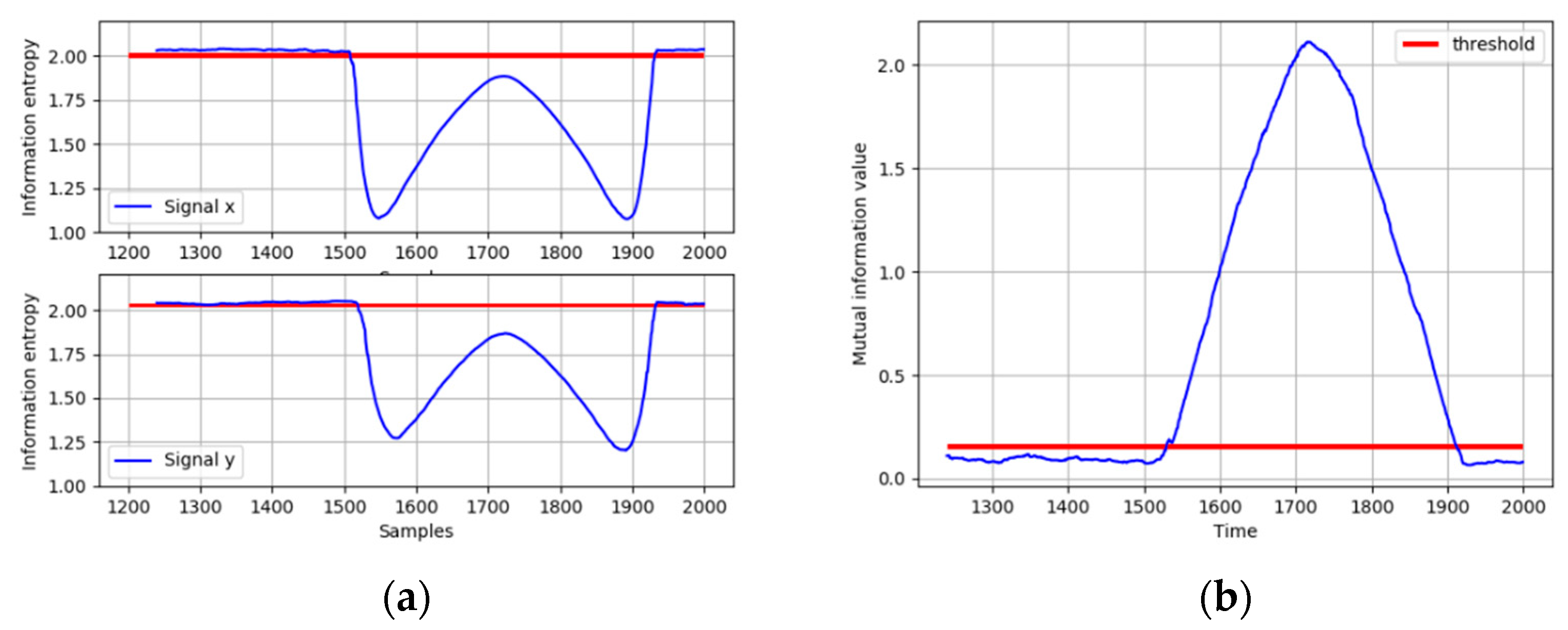
When the ramp fault occurs, the IE of
x and
y are calculated. As shown in
Figure 7a, both the IE of
x and
y decrease significantly and fall below the thresholds, indicating that the distributions of
x and
y both deviate from the normal operating condition. In order to diagnose the root cause of this fault, the MI between
x and
y is calculated and compared with its threshold. It can be seen from
Figure 7b that the MI between
x and
y exceeds its threshold when the fault occurs, which means that the fault could be propagated between
x and
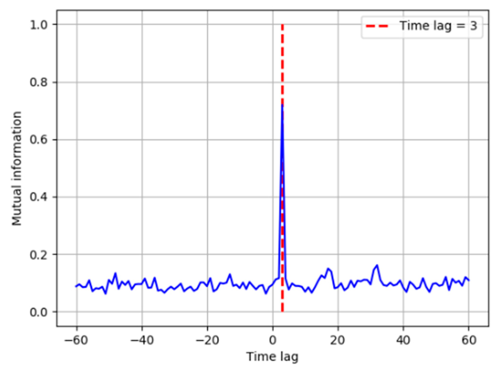
y. The direction of the interaction between
x and
y is identified based on the TDMI in
Figure 8. The time lag is introduced in
y, and it is obvious that the MI reaches its peak when the time lag is equal to 3, which means
y is caused by
x. Therefore, the fault propagation path can be easily determined as from
x to
y. The results show that the TDMI based method successfully identifies the root cause, together with its propagation path. Considering more numbers of process variables and more complicated variable correlation in industrial processes, the fault diagnosis results are displayed in the form of the directed graph in the following case studies.
5. Conclusions
In this work, variable correlation under normal operating conditions and faulty states is analyzed by MI. It can be concluded that variable correlation is mostly contributed from random noises under normal conditions. Once a faulty condition is detected, the true correlation can be identified if the fault is propagated between any two variables. Therefore, a fault diagnosis framework is proposed for fault propagation analysis and root cause identification. In steady state, correlation between each pair of variables caused by random noises is calculated to obtain a threshold. The fault propagation path is identified by TDMI between process variables using real-time data. The proposed method is applied to a simulated example, TEP, and an industrial process. The results show that not only can the fault propagation path be reasonably identified, but the root cause of faults can also be effectively isolated. It is worth noting that variable correlation under normal operation conditions can be different with that under faulty conditions in certain circumstances. The difference in variable correlation under different operation conditions can be effectively captured by the proposed method, which provides a more objective way to identify the fault propagation than previous fault diagnosis methods based on causal relations established by process knowledge or process data only under normal operating conditions. The logic of this fault diagnosis method can be applied to industrial processes with multiple operating conditions and complex control loops because variable correlation is solely captured from online data.
However, it is worth noticing that the calculation of TDMI is conducted by time-delayed windows among pair variables, by which the causal relations among them are determined. A certain propagation path may not be able to be identified if the sampling rate is slower than its propagation dynamic. In that case, both fast sampling rate and operator knowledge can help by proper integration of the proposed method in future study.


