
A Coupled CFD-DEM Model for Resolved Simulation of Filter Cake Formation during Solid-Liquid Separation


Abstract
1. Introduction
2. Materials and Methods
2.1. Filtration Equation
2.2. Filtration Experiments
2.3. Numerical Simulations
2.3.1. Fluid Flow Calculation with CFD
2.3.2. Particle Movement Calculation with DEM
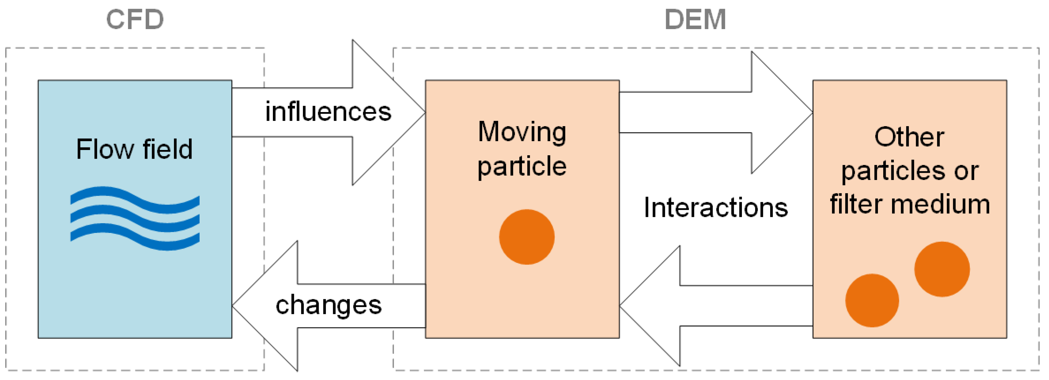
2.3.3. CFD-DEM Coupling
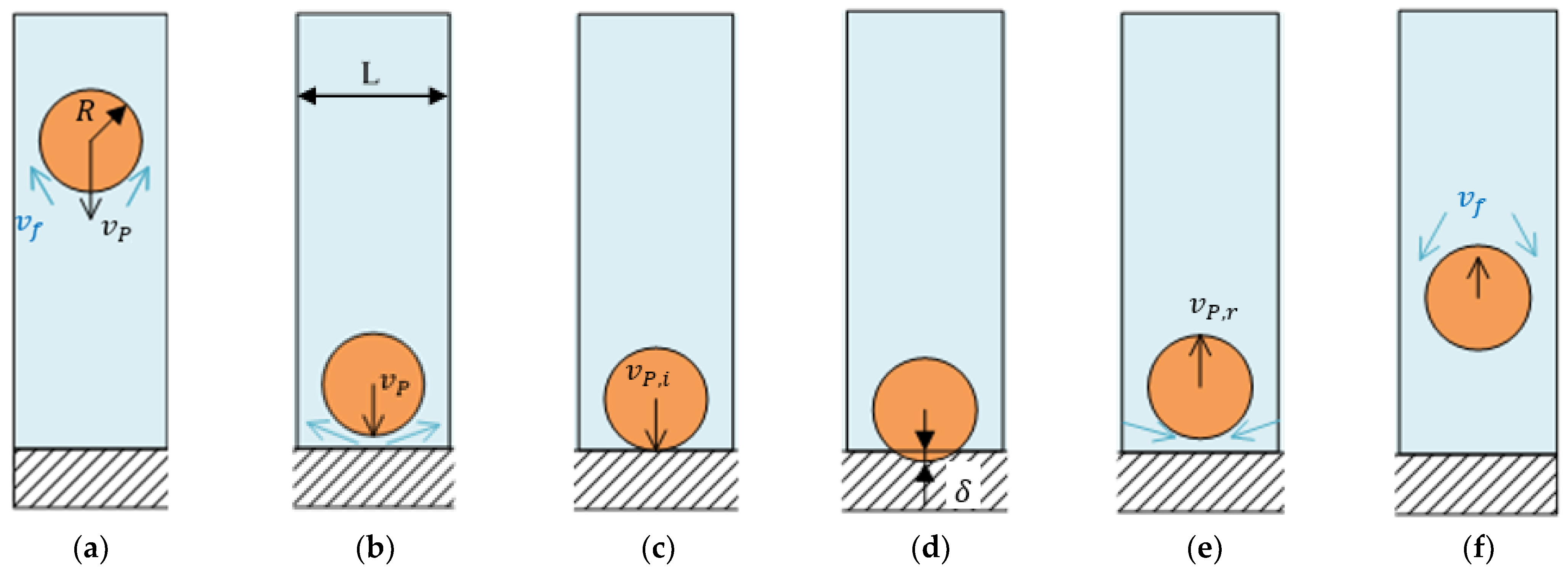
2.4. Particle Sedimentation
2.4.1. Theory
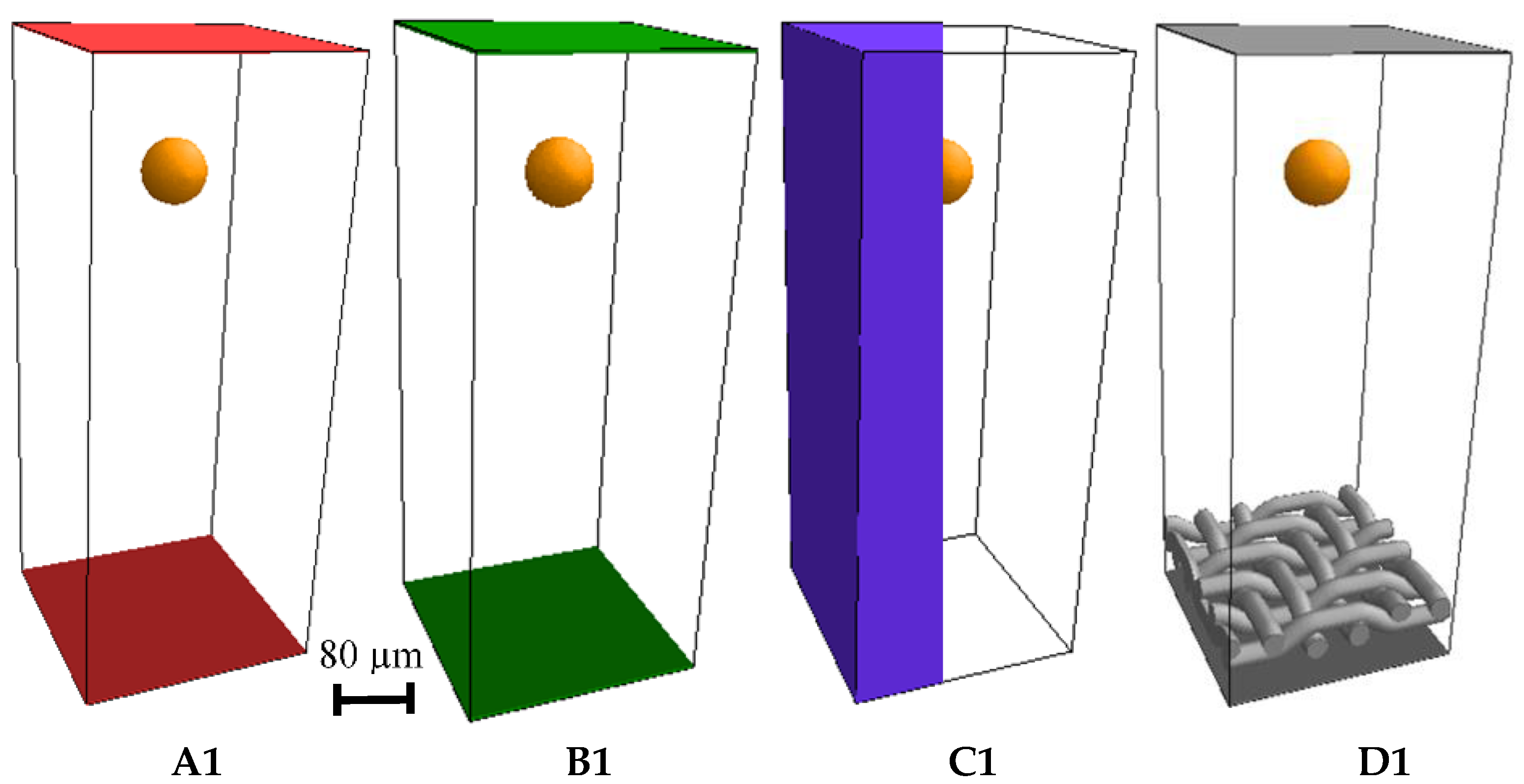
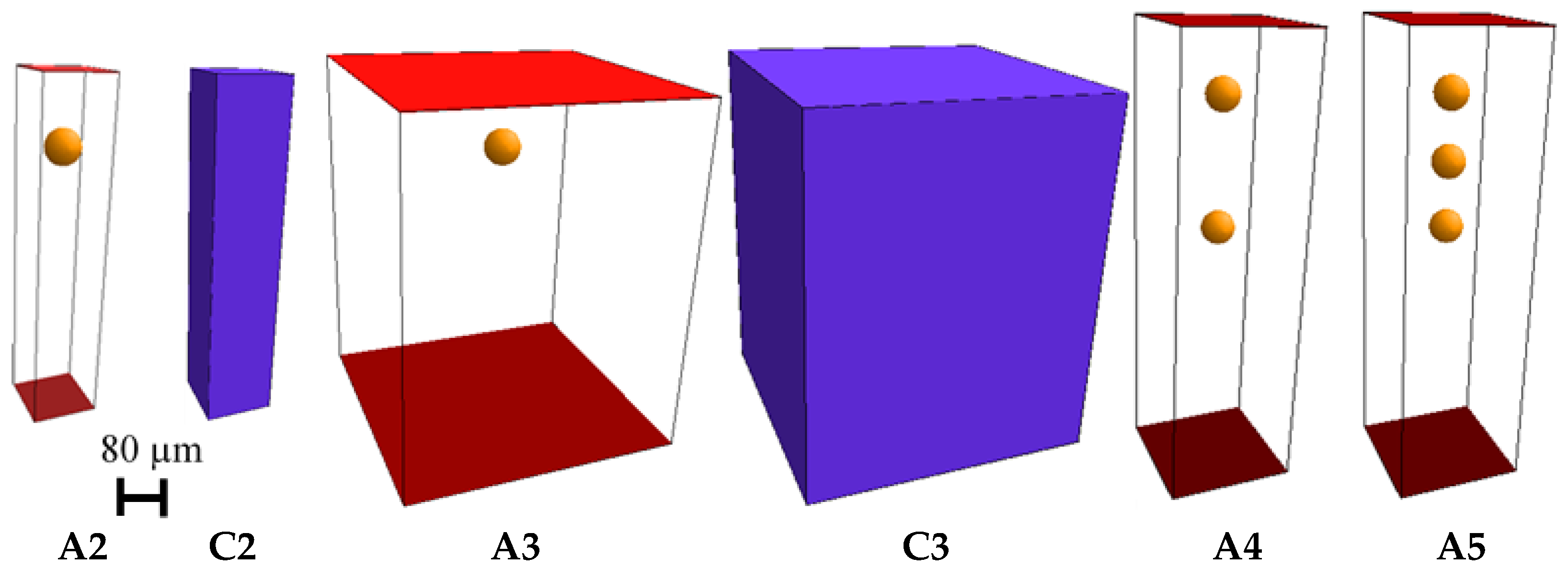
2.4.2. 3D Models
2.5. Separation Process
3. Results
3.1. Filtration Experiments
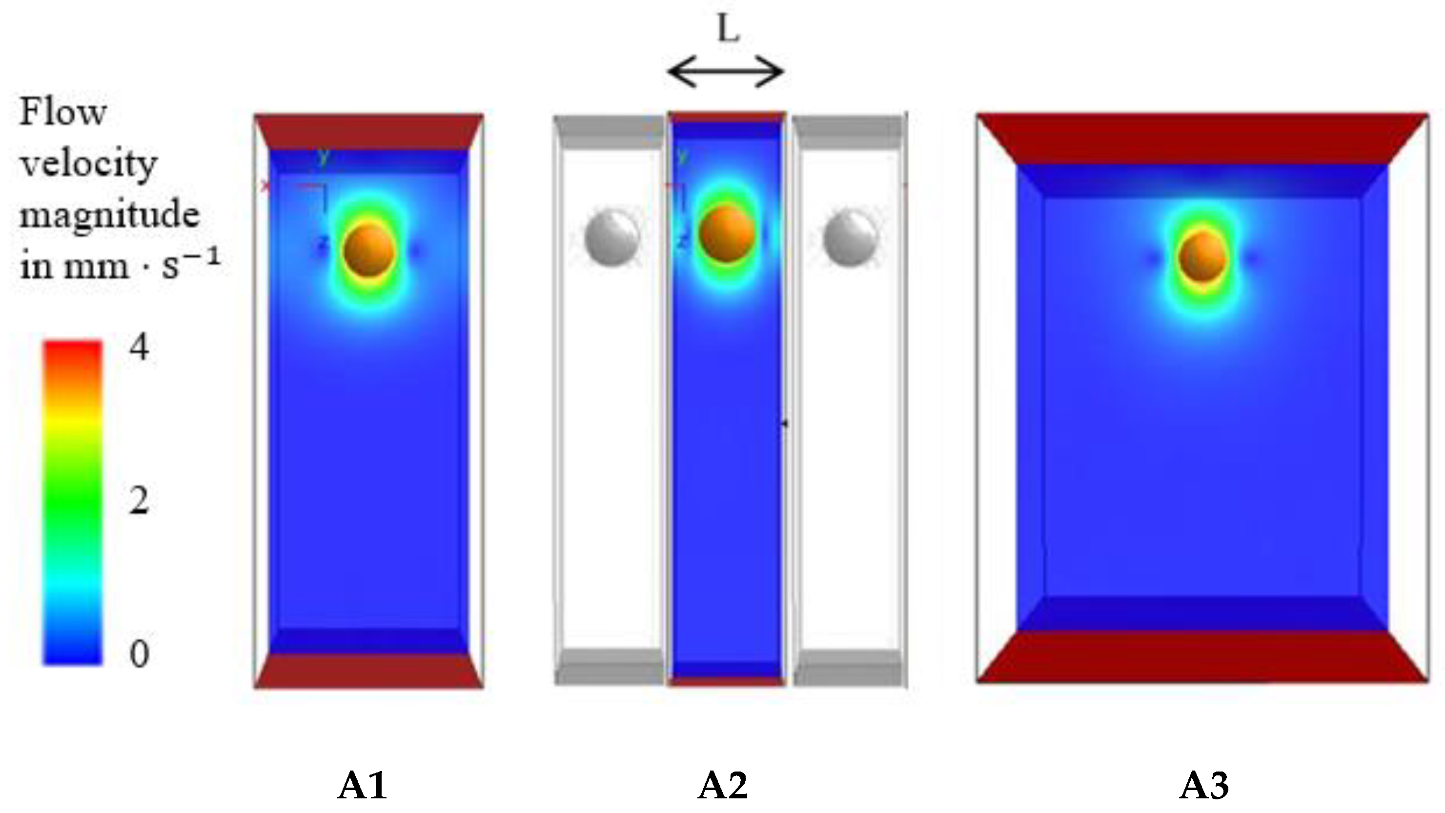
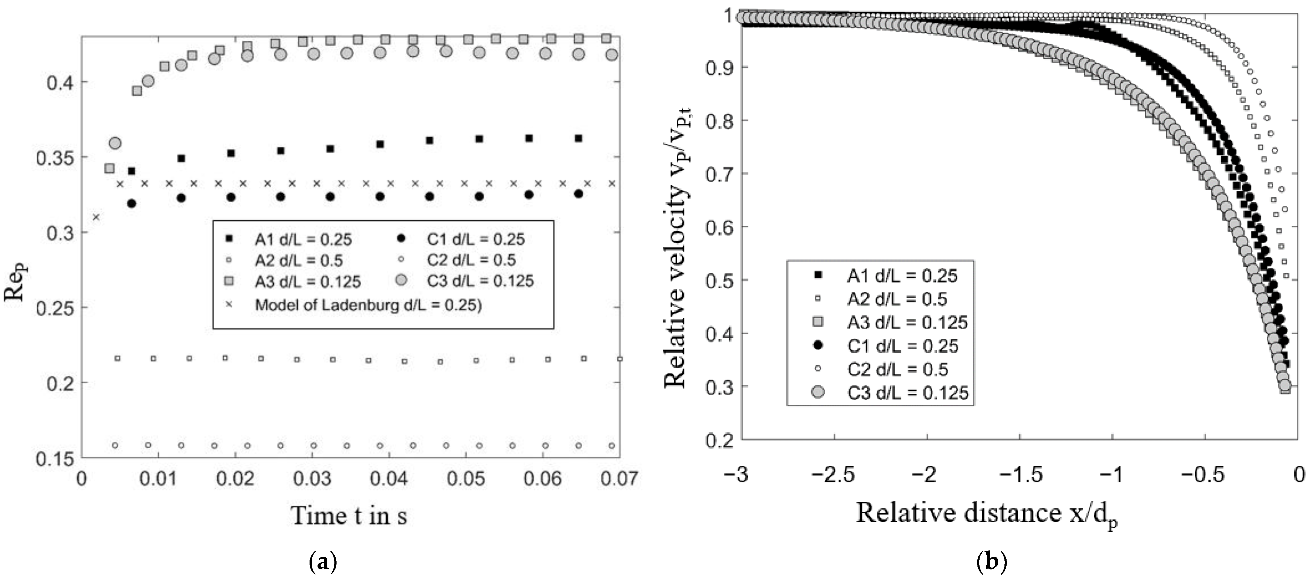
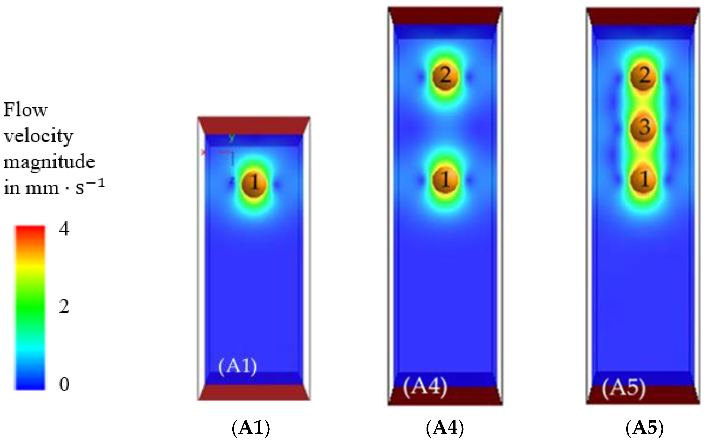
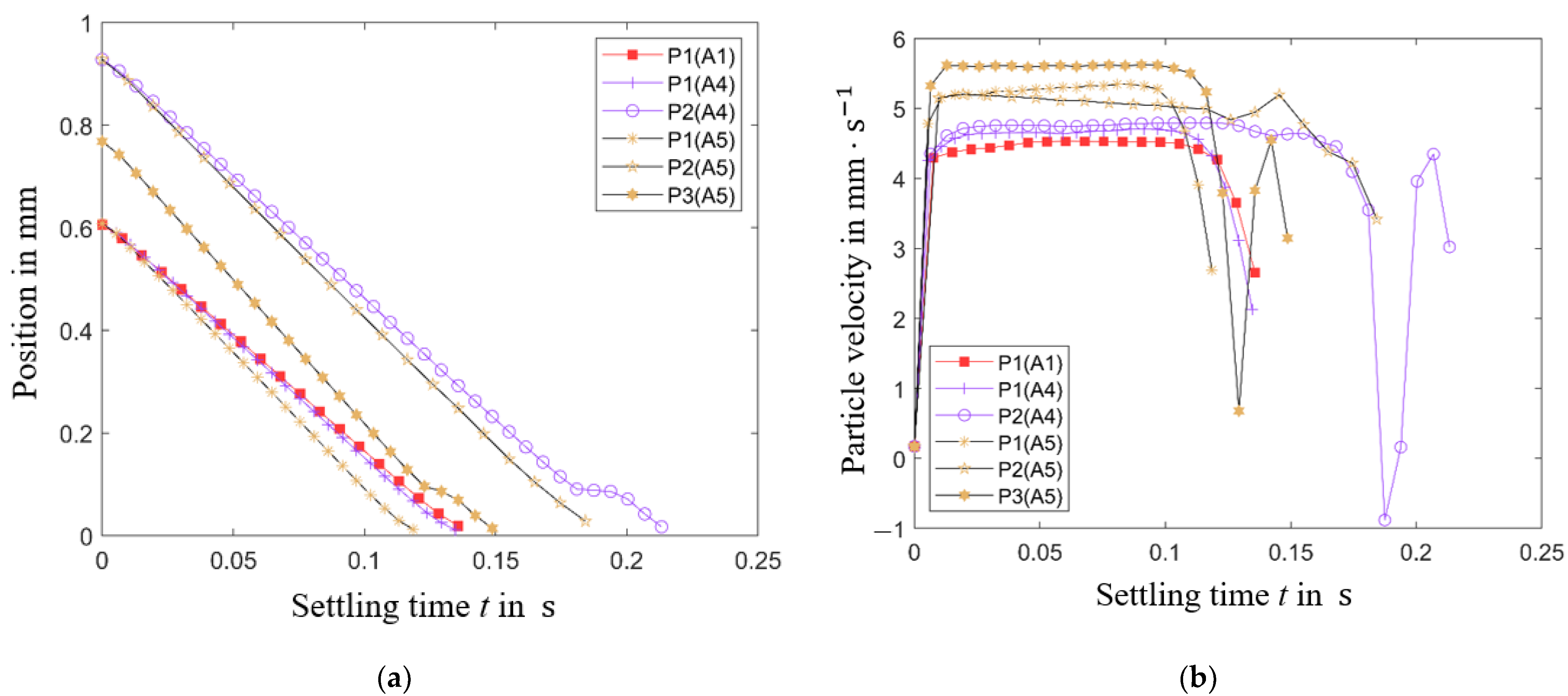
3.2. Simulation of the Particle Sedimentation
3.3. Simulation of the Filtration Process
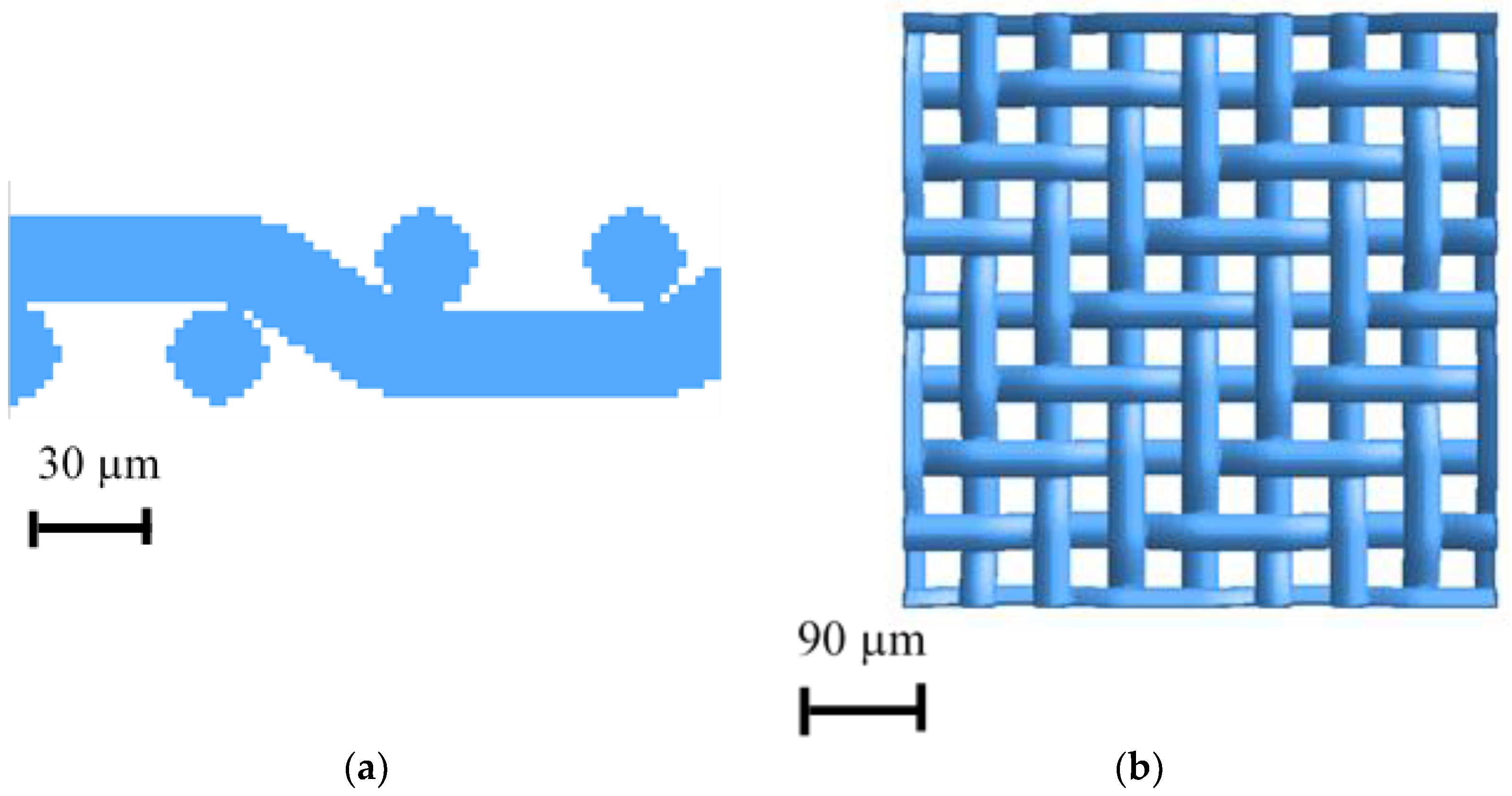
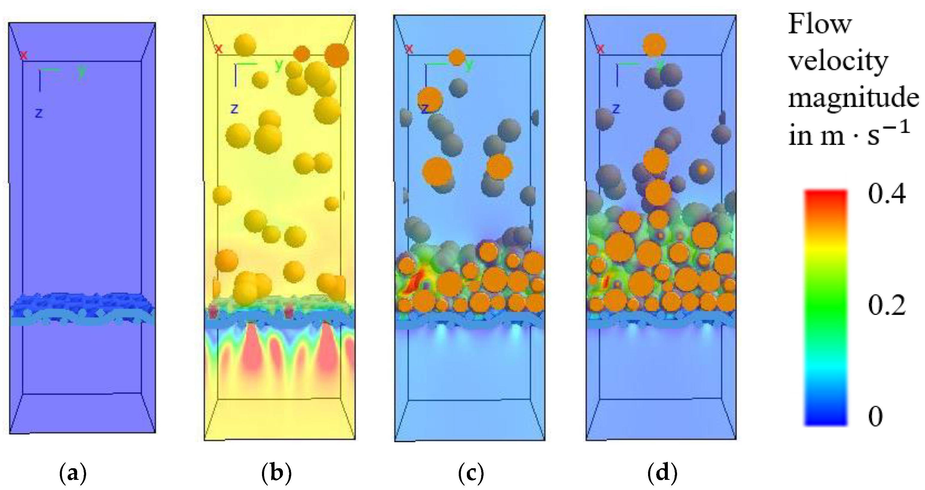
- In (a) the filter medium model is shown before the particle generation.
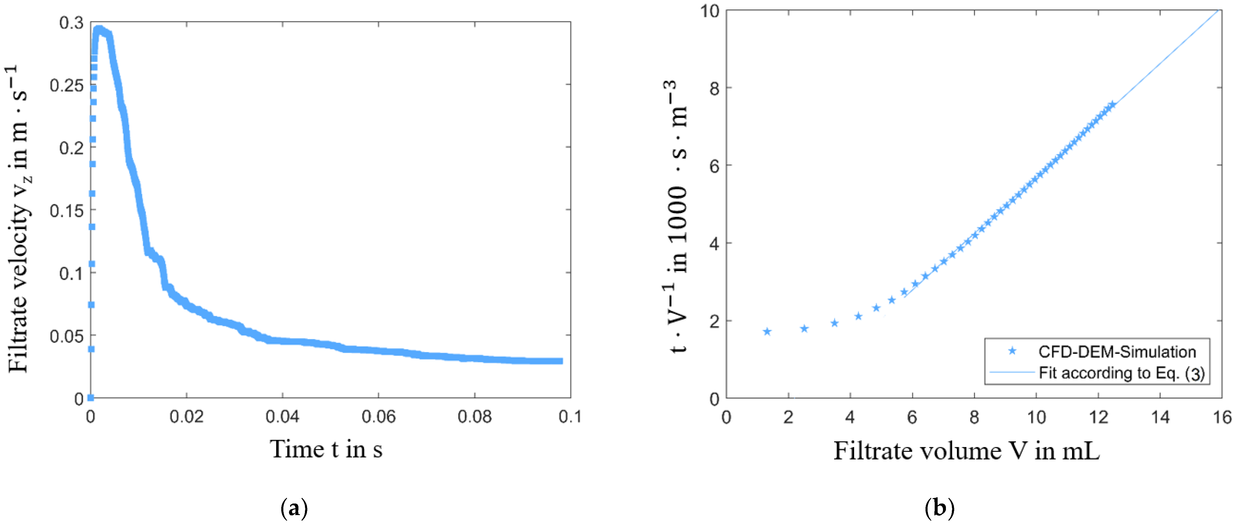
- In (b) the calculated flow velocities and the initial particle positions are shown at the beginning of the filtration when the first particles are reaching the filter medium and the fluid passes through the filter medium. The local flow velocity maxima in the area of the pores can be seen. Accordingly, the time-dependent filtrate velocity (Figure 19a) shows a maximum before this point of time because of the minimum pressure loss that is determined only by the filter medium.
- In (c) it can be seen that some particles are already clogging the pores of the filter medium, which leads to the increase of the pressure drop and the resulting decrease of the filtrate volume flow.
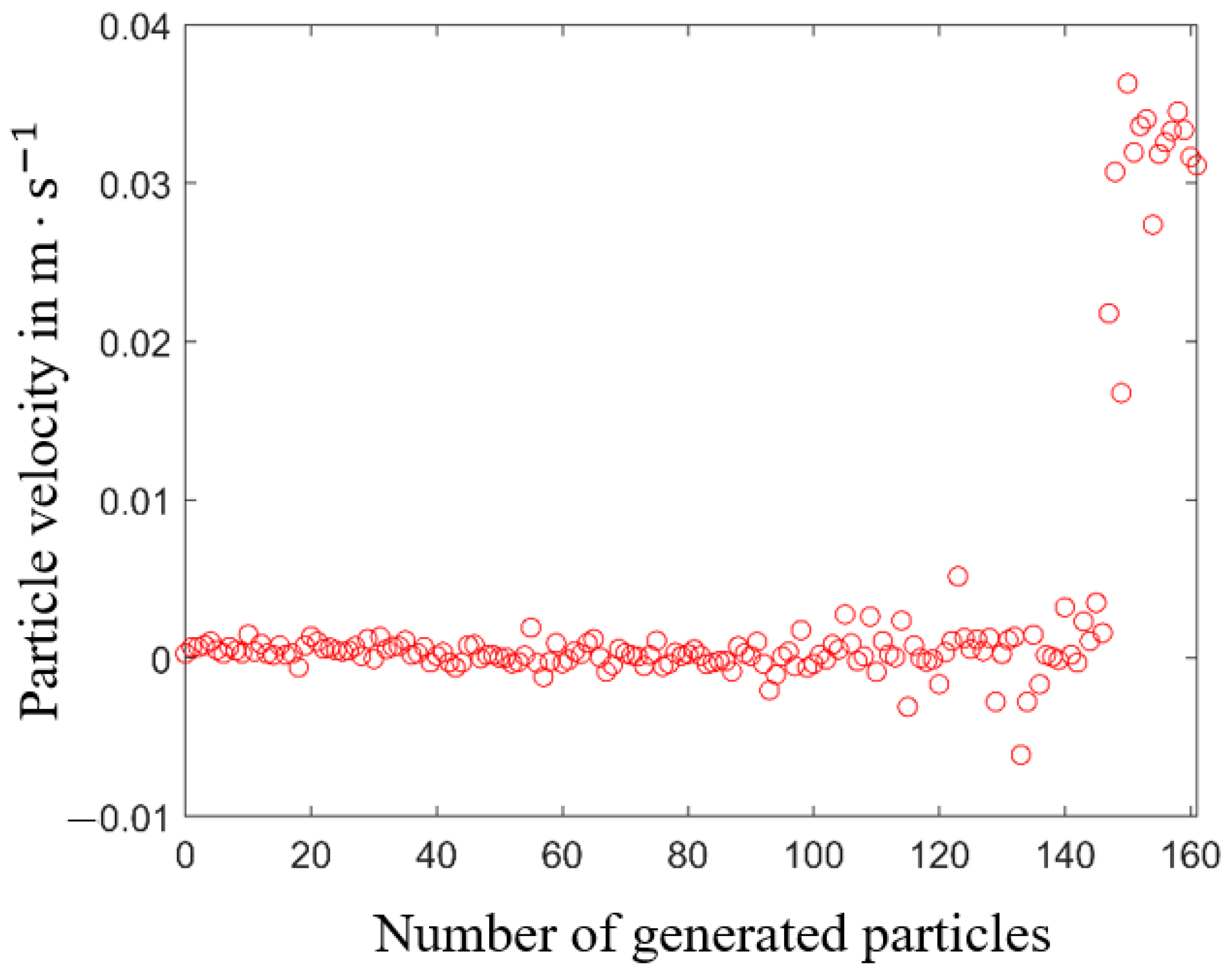
- In (d) the further filter cake formation process at the real time of 98 ms is shown. The filter cake height reaches 0.5 mm. It can be seen in Figure 20 that at this time point 145 particles have already been deposited in the filter cake and the other 16 generated particles are still settling. The particles in the filter cake do not remain fixed, some of them move slowly resulting in a reorganization and packing of the filter cake. These cake formation micro processes take place due to fluid flow, gravitation and contact forces between the particles.

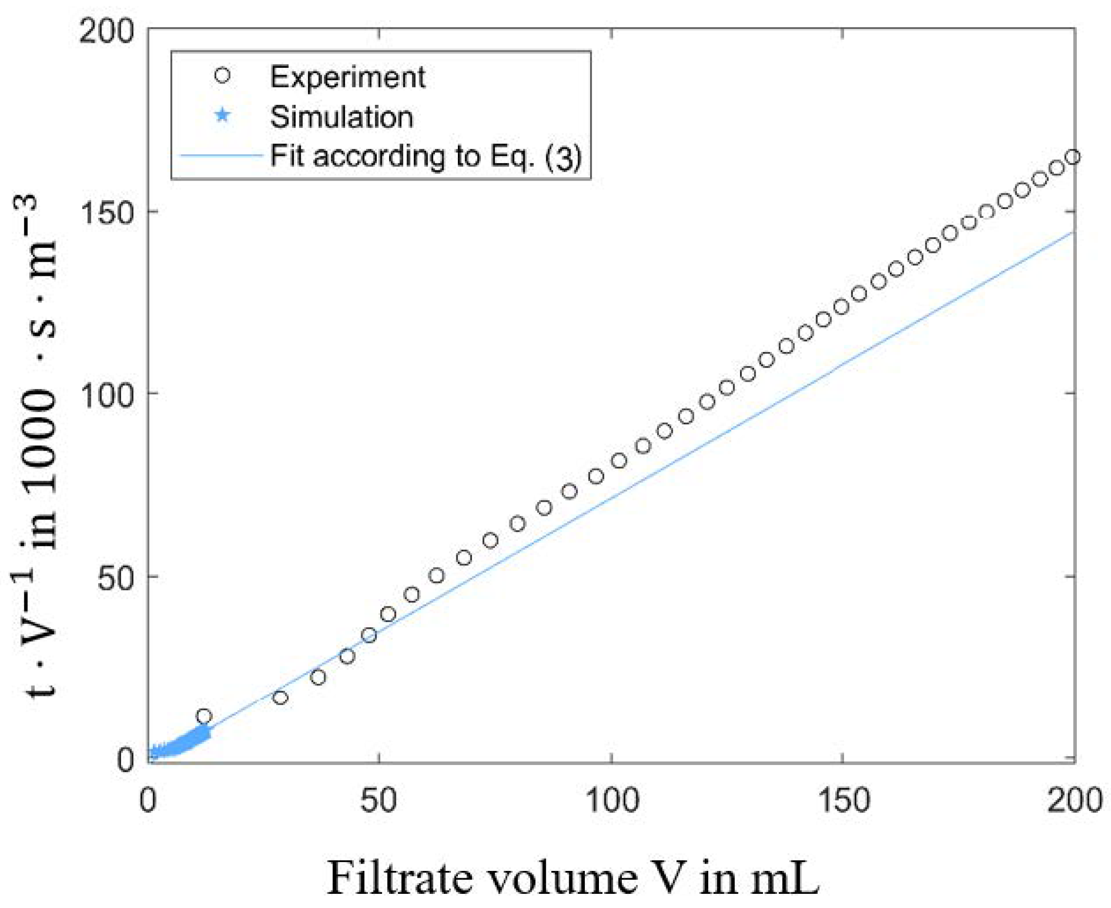
3.4. Comparison of Simulation and Experiment
4. Conclusions
Author Contributions
Funding
Institutional Review Board Statement
Informed Consent Statement
Data Availability Statement
Conflicts of Interest
References
- Ripperger, S.; Gösele, W.; Alt, C.; Loewe, T. Filtration, 1. Fundamentals. In Ullmann’s Encyclopedia of Industrial Chemistry; Wiley-VCH Verlag GmbH & Co. KgaA: Weinheim, Germany, 2013; pp. 1–38. ISBN 1435-6007. [Google Scholar] [CrossRef]
- Hund, D.; Lösch, P.; Kerner, M.; Ripperger, S.; Antonyuk, A. CFD-DEM study of bridging mechanisms at the static solid-liquid surface filtration. Powder Technol. 2020, 600–609. [Google Scholar] [CrossRef]
- Hund, D.; Schmidt, K.; Ripperger, S.; Antonyuk, S. Direct numerical simulation of cake formation during filtration with woven fabrics. Chem. Eng. Res. Des. 2018, 139, 26–33. [Google Scholar] [CrossRef]
- Lösch, P.; Nikolaus, K.; Antonyuk, S. Fractionating of finest particles using cross-flow separation with superimposed electric field. Sep. Purif. Technol. 2021, 257, 117820. [Google Scholar] [CrossRef]
- Kerner, M.; Schmidt, K.; Hellmann, A.; Schumacher, S.; Pitz, M.; Asbach, C.; Ripperger, S.; Antonyuk, S. Numerical and experimental study of submicron aerosol deposition in electret microfiber nonwovens. J. Aerosol Sci. 2018, 122, 32–44. [Google Scholar] [CrossRef]
- Kerner, M.; Schmidt, K.; Schumacher, S.; Puderbach, V.; Asbach, C.; Antonyuk, S. Evaluation of electrostatic properties of electret filters for aerosol deposition. Sep. Purif. Technol. 2020, 239, 116548. [Google Scholar] [CrossRef]
- Hosseini, S.A.; Tafreshi, H.V. 3-D simulation of particle filtration in electrospun nanofibrous filters. Powder Technol. 2010, 201, 153–160. [Google Scholar] [CrossRef]
- Brauer, H. Grundlagen der Einphasen- und Mehrphasenströmungen; Sauerländer: Aarau, Switzerland, 1971. [Google Scholar]
- Sommerfeld, M.; Horender, S. Fluid Mechanics. Ullmann’s Encyclopedia of Industrial Chemistry; Wiley-VCH Verlag GmbH & Co. KGaA: Weinheim, Germany, 2012. [Google Scholar]
- Wakeman, R. The influence of particle properties on filtration. Sep. Purif. Technol. 2007, 58, 234–241. [Google Scholar] [CrossRef]
- Anlauf, H. Wet Cake Filtration: Fundamentals, Equipment, Strategies; Wiley-VCH Verlag GmbH & Co. KGaA: Weinheim, Germany, 2020; ISBN 3527346066. [Google Scholar]
- Hieke, M.; Nirschl, H. Einfluss der Salzkonzentration auf das rheologische Verhalten wässriger anorganischer Suspensionen bei der Filtration. Chem. Ing. Tech. 2007, 79, 1939–1944. [Google Scholar] [CrossRef][Green Version]
- Cundall, P.A.; Strack, O.D.L. A discrete numerical model for granular assemblies. Géotechnique 1979, 29, 47–65. [Google Scholar] [CrossRef]
- Guo, Y.; Curtis, J.S. Discrete Element Method Simulations for Complex Granular Flows. Annu. Rev. Fluid Mech. 2015, 47, 21–46. [Google Scholar] [CrossRef]
- Pöschel, T.; Schwager, T. Computational Granular Dynamics: Models and Algorithms; Springer: Berlin, Germany, 2005; ISBN 9783540277200. [Google Scholar]
- Zhong, W.; Yu, A.; Liu, X.; Tong, Z.; Zhang, H. DEM/CFD-DEM Modelling of Non-spherical Particulate Systems: Theoretical Developments and Applications. Powder Technol. 2016, 302, 108–152. [Google Scholar] [CrossRef]
- Antonyuk, S.; Khanal, M.; Tomas, J.; Heinrich, S.; Mörl, L. Impact breakage of spherical granules: Experimental study and DEM simulation. Chem. Eng. Process. Process Intensif. 2006, 45, 838–856. [Google Scholar] [CrossRef]
- Qian, F.; Huang, N.; Lu, J.; Han, Y. CFD–DEM simulation of the filtration performance for fibrous media based on the mimic structure. Comput. Chem. Eng. 2014, 71, 478–488. [Google Scholar] [CrossRef]
- Breuninger, P.; Weis, D.; Behrendt, I.; Grohn, P.; Krull, F.; Antonyuk, S. CFD–DEM simulation of fine particles in a spouted bed apparatus with a Wurster tube. Particuology 2019, 42, 114–125. [Google Scholar] [CrossRef]
- Riefler, N.; Ulrich, M.; Morshäuser, M.; Fritsching, U. Particle penetration in fiber filters. Particuology 2018, 40, 70–79. [Google Scholar] [CrossRef]
- Volk, A.; Ghia, U.; Stoltz, C. Effect of grid type and refinement method on CFD-DEM solution trend with grid size. Powder Technol. 2017, 311, 137–146. [Google Scholar] [CrossRef]
- Vångö, M.; Pirker, S.; Lichtenegger, T. Unresolved CFD–DEM modeling of multiphase flow in densely packed particle beds. Appl. Math. Model. 2018, 56, 501–516. [Google Scholar] [CrossRef]
- Zhao, J.; Shan, T. Coupled CFD–DEM simulation of fluid–particle interaction in geomechanics. Powder Technol. 2013, 239, 248–258. [Google Scholar] [CrossRef]
- Deshpande, R.; Antonyuk, S.; Iliev, O. Study of the filter cake formed due to the sedimentation of monodispersed and bidispersed particles using discrete element method-computational fluid dynamics simulations. AIChE J. 2019, 65, 1294–1303. [Google Scholar] [CrossRef]
- Deshpande, R. Investigation of the Filter Cake Formation Process using DEM-CFD Simulation with Experimentally Calibrated Parameters; Fraunhofer Verlag: Stuttgart, Germany, 2019; ISBN 3839615194. [Google Scholar]
- Joseph, G.G.; Zenit, R.; Hunt, M.L.; Rosenwinkel, A.M. Particle–wall collisions in a viscous fluid. J. Fluid Mech. 2001, 433, 329–346. [Google Scholar] [CrossRef]
- Heuzeroth, F.; Fritzsche, J.; Werzner, E.; Mendes, M.A.A.; Ray, S.; Trimis, D.; Peuker, U.A. Viscous force—An important parameter for the modeling of deep bed filtration in liquid media. Powder Technol. 2015, 283, 190–198. [Google Scholar] [CrossRef]
- Wang, L.; Guo, Z.L.; Mi, J.C. Drafting, kissing and tumbling process of two particles with different sizes. Comput. Fluids 2014, 96, 20–34. [Google Scholar] [CrossRef]
- Krause, M.J.; Klemens, F.; Henn, T.; Trunk, R.; Nirschl, H. Particle flow simulations with homogenised lattice Boltzmann methods. Particuology 2017, 34, 1–13. [Google Scholar] [CrossRef]
- Deen, N.G.; van Sint Annaland, M.; van der Hoef, M.A.; Kuipers, J.A.M. Review of discrete particle modeling of fluidized beds. Chem. Eng. Sci. 2007, 62, 28–44. [Google Scholar] [CrossRef]
- Golshan, S.; Sotudeh-Gharebagh, R.; Zarghami, R.; Mostoufi, N.; Blais, B.; Kuipers, J.A.M. Review and implementation of CFD-DEM applied to chemical process systems. Chem. Eng. Sci. 2020, 221, 115646. [Google Scholar] [CrossRef]
- Cook, B.K.; Noble, D.R.; Williams, J.R. A direct simulation method for particle-fluid systems. Eng. Comput. 2004, 21, 151–168. [Google Scholar] [CrossRef]
- Third, J.R.; Chen, Y.; Müller, C.R. Comparison between finite volume and lattice-Boltzmann method simulations of gas-fluidised beds: Bed expansion and particle–fluid interaction force. Comput. Part. Mech. 2016, 3, 373–381. [Google Scholar] [CrossRef]
- Brumby, P.E.; Sato, T.; Nagao, J.; Tenma, N.; Narita, H. Coupled LBM–DEM Micro-scale Simulations of Cohesive Particle Erosion Due to Shear Flows. Transp. Porous Media 2015, 109, 43–60. [Google Scholar] [CrossRef]
- Zhang, C.; Soga, K.; Kumar, K.; Sun, Q.; Jin, F. Numerical study of a sphere descending along an inclined slope in a liquid. Granul. Matter 2017, 19. [Google Scholar] [CrossRef]
- Li, B.; Zhang, S.-B.; Teng, Z.-Y.; Bian, Y.-M.; Zhang, J.; Ba, X.-Y. Mesoscale simulation and analysis of spouted bed with LBM-DEM four direction coupling. Jisuan Lixue Xuebao/Chin. J. Comput. Mech. 2018, 35, 527–532. [Google Scholar] [CrossRef]
- Xiong, Q.; Madadi-Kandjani, E.; Lorenzini, G. A LBM–DEM solver for fast discrete particle simulation of particle–fluid flows. Contin. Mech. Thermodyn. 2014, 26, 907–917. [Google Scholar] [CrossRef]
- Kuruneru, S.T.W.; Marechal, E.; Deligant, M.; Khelladi, S.; Ravelet, F.; Saha, S.C.; Sauret, E.; Gu, Y. A Comparative Study of Mixed Resolved–Unresolved CFD-DEM and Unresolved CFD-DEM Methods for the Solution of Particle-Laden Liquid Flows. Arch. Comput. Methods Eng. 2019, 26, 1239–1254. [Google Scholar] [CrossRef]
- Rettinger, C.; Rüde, U. A coupled lattice Boltzmann method and discrete element method for discrete particle simulations of particulate flows. Comput. Fluids 2018, 172, 706–719. [Google Scholar] [CrossRef]
- Rettinger, C.; Rüde, U. Dynamic Load Balancing Techniques for Particulate Flow Simulations. Computation 2019, 7, 9. [Google Scholar] [CrossRef]
- Stiess, M. Mechanische Verfahrenstechnik 2; Springer Berlin Heidelberg: Heidelberg, Germany, 1997; ISBN 978-3-662-08599-8. [Google Scholar]
- Tichy, J.W. Zum Einfluss des Filtermittels und der Auftretenden Interferenzen Zwischen Filterkuchen und Filtermittel bei der Kuchenfiltration. Ph.D. Dissertation, Technische Universität Kaiserslautern, Kaiserslautern, Germany, 2007. Available online: https://kluedo.ub.uni-kl.de/frontdoor/index/index/docId/1856 (accessed on 9 May 2021).
- Verein Deutscher Ingenieure e.V. VDI 2762: Filtrierbarkeit von Suspensionen Bestimmung des Filterkuchenwiderstands. VDI Richtline. In VDI-Handbuch Verfahrenstechnik und Chemieingenieurwesen, Band 5: Spezielle Verfahrenstechniken; Verein Deutscher Ingenieure e.V.: Düsseldorf, Germany, 2010. [Google Scholar]
- Junk, M.; Yong, W.-A. Rigorous Navier-Stokes Limit of the Lattice Boltzmann Equation; Berichte der Arbeitsgruppe Technomathematik (AGTM Report)—243. Available online: https://kluedo.ub.uni-kl.de/frontdoor/index/index/docId/1273 (accessed on 9 May 2021).
- Thömmes, G.; Becker, J.; Junk, M.; Vaikuntam, A.K.; Kehrwald, D.; Klar, A.; Steiner, K.; Wiegmann, A. A Lattice Boltzmann Method for Immiscible Multiphase Flow Simulations Using the Level Set Method; Berichte des Fraunhofer ITWM No. 134. 2008. Available online: https://kluedo.ub.uni-kl.de/frontdoor/index/index/docId/1989 (accessed on 9 May 2021).
- Gervais, P.-C.; Bémer, D.; Bourrous, S.; Ricciardi, L. Airflow and particle transport simulations for predicting permeability and aerosol filtration efficiency in fibrous media. Chemical Engineering Science 2017, 165, 154–164. [Google Scholar] [CrossRef]
- Mohamad, A.A. Lattice Boltzmann Method: Fundamentals and Engineering Applications with Computer Codes, 2nd ed.; Springer-Verlag: London, UK, 2019. [Google Scholar] [CrossRef]
- Hertz, H. Über die Berührung fester elastischer Körper. J. Die Reine Angew. Math. 1881, 92, 156–171. [Google Scholar]
- Langston, P.A.; Tüzün, U.; Heyes, D.M. Discrete element simulation of granular flow in 2D and 3D hoppers: Dependence of discharge rate and wall stress on particle interactions. Chem. Eng. Sci. 1995, 50, 967–987. [Google Scholar] [CrossRef]
- Stiess, M. Mechanische Verfahrenstechnik—Partikeltechnologie 1; Springer Berlin Heidelberg: Berlin/Heidelberg, Germany, 2009; ISBN 978-3-540-32551-2. [Google Scholar]
- Fidleris, V.; Whitmore, R.L. Experimental Determination of Wall Effect for Spheres Falling Axially in Cylindrical Vessels. British J. Appl. Phys. 1961, 12, 490. [Google Scholar] [CrossRef]
- Brown, P.P.; Lawler, D.F. Sphere Drag and Settling Velocity Revisited. J. Environ. Eng. 2003, 129, 222–231. [Google Scholar] [CrossRef]
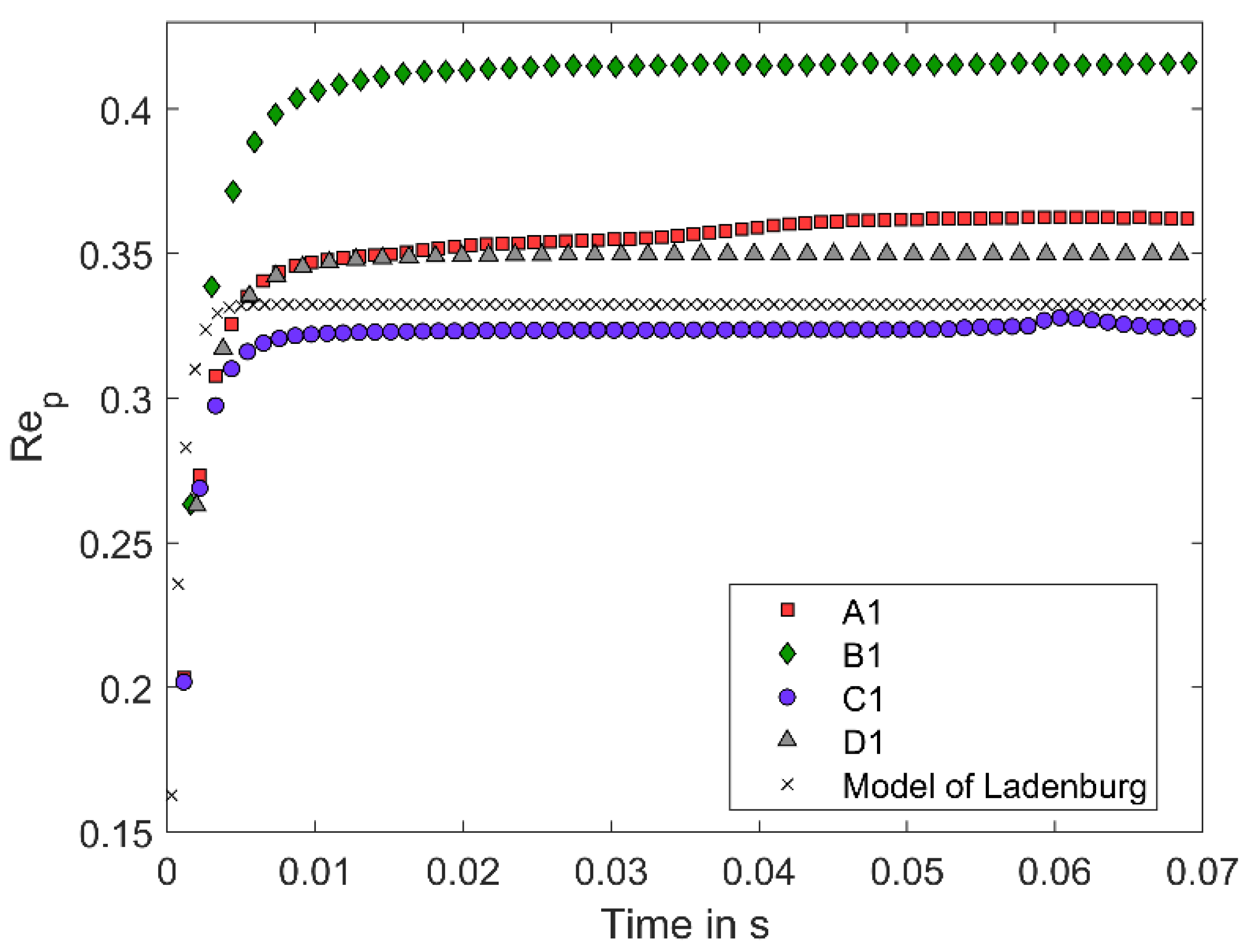
- Ladenburg, R. Über den Einfluß von Wänden auf die Bewegung einer Kugel in einer reibenden Flüssigkeit. Ann. Phys. 1907, 328, 447–458. [Google Scholar] [CrossRef]
- Rettinger, C.; Rüde, U. An Efficient Four-Way Coupled Lattice Boltzmann—Discrete Element Method for Fully Resolved Simulations of Particle-Laden Flows. arXiv 2020, arXiv:2003.01490. Available online: https://arxiv.org/pdf/2003.01490 (accessed on 9 May 2021).


| Property | Unit | Value |
|---|---|---|
| mesh size | µm | 32 |
| wire diameter | µm | 28 |
| filter area | cm2 | 20 |
| pressure difference | Pa | 1000 |
| particle density | kg∙m−3 | 2200 |
| particle size median value | µm | 82.2 |
| particle size modal value | µm | 82.7 |
| x10,3 1 | µm | 69.6 |
| x90,3 2 | µm | 95.3 |
| Property | Unit | Model | Value |
|---|---|---|---|
| Voxel length | µm | A1, A2, A3, A4, A5, C1, C2, C3, D1 | 2 |
| B1 | 4 | ||
| Model size (L × W × H) | µm × µm × µm | A1, C1, D1 | 320 × 320 × 802 |
| A2, C2 | 160 × 160 × 802 | ||
| A3, C3 | 640 × 640 × 802 | ||
| A4, A5 | 320 × 320 × 1128 | ||
| B1 | 320 × 320 × 804 | ||
| Wire diameter | µm | D1 | 28 |
| Pore size | µm | D1 | 32 |
| Particle density | kg∙m−3 | every model | 2200 |
| Particle diameter | µm | every model | 80 |
| Fluid density | kg∙m−3 | every model | 1000 |
| Fluid viscosity | Pa∙s | every model | 0.001 |
| Number of particles | - | A1, A2, A3, B1, C1, C2, C3, D1 | 1 |
| A4 | 2 | ||
| A5 | 3 | ||
| Ratio | - | A1, B1, C1, D1, A4, A5 | 0.25 |
| A2, C2 | 0.5 | ||
| A3, C3 | 0.125 |
| Property | Unit | Value |
|---|---|---|
| Voxel length | µm | 2.5 |
| Wire diameter | µm | 28 |
| Pore size | µm | 32 |
| Particle density | kg∙m−3 | 2200 |
| Particle diameter of the generated fractions | µm | 55 |
| 63 | ||
| 72 | ||
| 83 | ||
| 95 | ||
| 109 | ||
| Particle concentration | m−3 | 1011 |
| Pressure difference | Pa | 1000 |
| Fluid density | kg∙m−3 | 1000 |
| Fluid viscosity | Pa∙s | 0.001 |
Publisher’s Note: MDPI stays neutral with regard to jurisdictional claims in published maps and institutional affiliations. |
© 2021 by the authors. Licensee MDPI, Basel, Switzerland. This article is an open access article distributed under the terms and conditions of the Creative Commons Attribution (CC BY) license (https://creativecommons.org/licenses/by/4.0/).
Share and Cite
Puderbach, V.; Schmidt, K.; Antonyuk, S. A Coupled CFD-DEM Model for Resolved Simulation of Filter Cake Formation during Solid-Liquid Separation. Processes 2021, 9, 826. https://doi.org/10.3390/pr9050826
Puderbach V, Schmidt K, Antonyuk S. A Coupled CFD-DEM Model for Resolved Simulation of Filter Cake Formation during Solid-Liquid Separation. Processes. 2021; 9(5):826. https://doi.org/10.3390/pr9050826
Chicago/Turabian StylePuderbach, Vanessa, Kilian Schmidt, and Sergiy Antonyuk. 2021. "A Coupled CFD-DEM Model for Resolved Simulation of Filter Cake Formation during Solid-Liquid Separation" Processes 9, no. 5: 826. https://doi.org/10.3390/pr9050826
APA StylePuderbach, V., Schmidt, K., & Antonyuk, S. (2021). A Coupled CFD-DEM Model for Resolved Simulation of Filter Cake Formation during Solid-Liquid Separation. Processes, 9(5), 826. https://doi.org/10.3390/pr9050826