Model-Based Design of Experiments for High-Dimensional Inputs Supported by Machine-Learning Methods

Abstract

Algorithms that compute locally optimal continuous designs often rely on a finite design space or on the repeated solution of difficult non-linear programs. Both approaches require extensive evaluations of the Jacobian $Df$ of the underlying model. These evaluations are a heavy computational burden. Based on the Kiefer-Wolfowitz Equivalence Theorem, we present a novel design of experiments algorithm that computes optimal designs in a continuous design space. For this iterative algorithm, we combine an adaptive Bayes-like sampling scheme with Gaussian process regression to approximate the directional derivative of the design criterion. The approximation allows us to adaptively select new design points on which to evaluate the model. The adaptive selection of the algorithm requires significantly less evaluations of $Df$ and reduces the runtime of the computations. We show the viability of the new algorithm on two examples from chemical engineering.

1. Introduction

In chemical engineering, the use of models is indispensable to describe, design and optimize processes—both on a lab and on production scales, both with academic and with industrial backgrounds. However, each model prediction is only as good as the model, which means that the reliability of models to describe and predict the outcome of real-world processes is crucial.

A precise model $f:X\to Y$ gives a good understanding of the underlying phenomenon and is the basis for reliable simulation and optimization results. These models often depend on a variety of parameters $\theta$ that need to be estimated from measured data. Therefore, experiments were performed and measurements were taken in order to obtain a good estimate. Ideally, these experiments should be as informative as possible, such that the estimate of the model parameters is most accurate within the measurement errors.

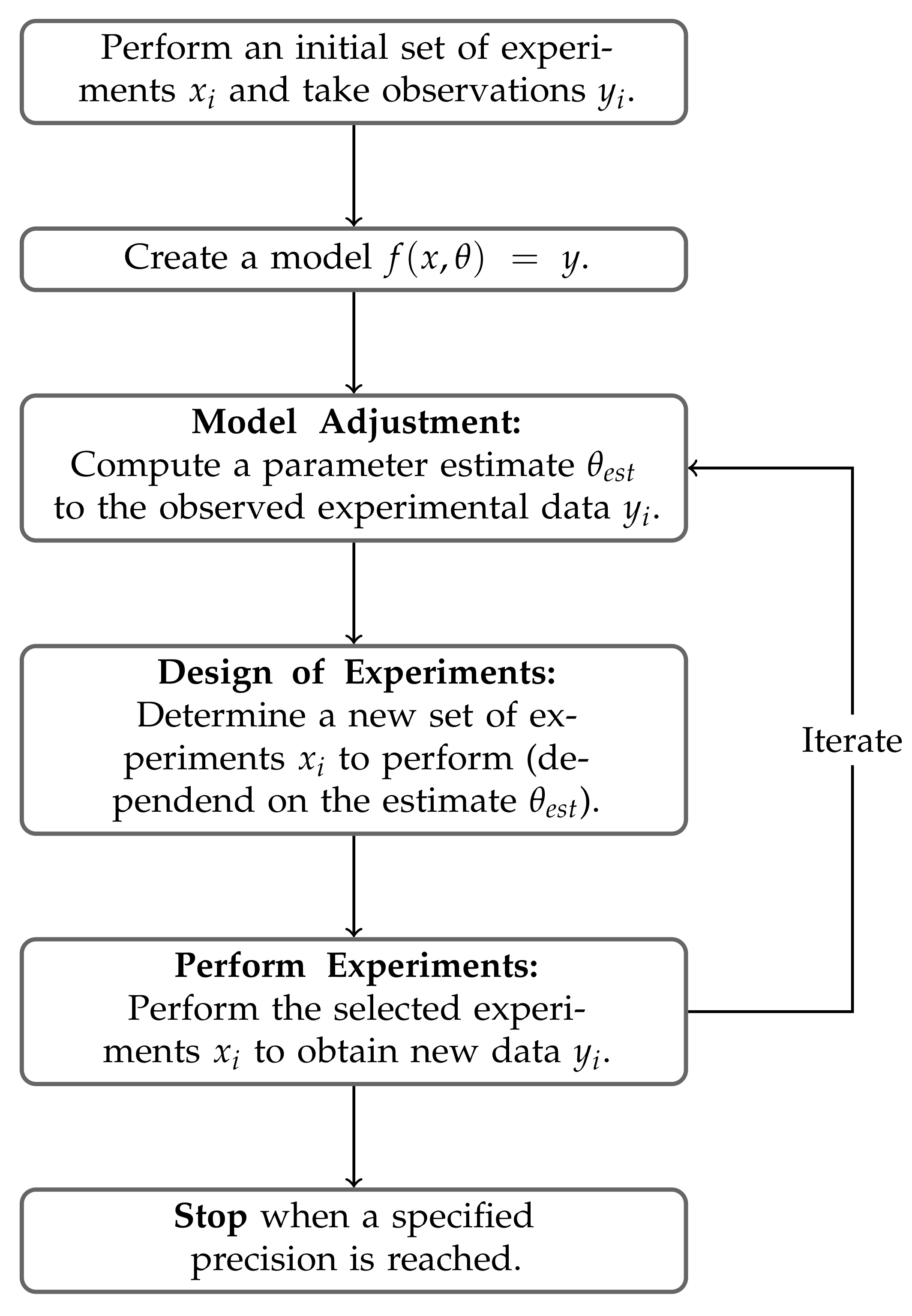
A common approach is an iterative workflow, which is presented in Figure 1. One begins by performing an initial set of experiments and measures corresponding results. With this data, a model $f(x,\theta )$ that describes the experiments was constructed. Additionally, an estimate ${\theta }_{est}$ of the unknown parameters $\theta$ was computed (model adjustment). The next step was to find a new set of experiments to perform. Finding appropriate experiments is the subject of the model-based design of experiments (MbDoE), also called optimal experimental design (OED). The new experiments were performed and new data were collected. The process of adjusting the model parameters, determining experiments and performing these experiments is iterated until one is satisfied with the parameter estimate ${\theta }_{est}$. A detailed overview on this iterative model identification workflow and each individual step can be found in [1] or [2,3,4].

In the model-based design of experiments, the current information of the model is used in order to find optimal experiments. Here, optimal means finding experiments that give the most information on the unknown parameters $\theta$. Equivalently, the error (variance) of the estimate ${\theta }_{est}$ is minimized [1,5,6,7]. MbDoE has been considered for a variety of minimization criteria of the variance [1] as well as for a variety of model types. These include non-linear models, multi-response models and models with distributional assumptions on the observations—see [1]. More recently dynamical models $y\left(t\right)=f\left(x\right(t),\theta )$—possibly given via differential equations $0=g(\dot{x}\left(t\right),x\left(t\right),\theta )$—have also gained more traction in MbDoE—see [2,8,9,10]. Duarte et al. proposed a formulation for implicit models $f(x,y,\theta )=0$ in [11].

The computed optimal designs will depend on the information currently available from the model. In particular, they depend on the current estimate ${\theta }_{est}$ of the unknown parameters $\theta$. Such designs are called locally optimal. In contrast, one can also compute robust optimal designs that take the uncertainty of the current estimate ${\theta }_{est}$ into account. Such robust designs are often used in the initial iteration, when no estimate of the parameters is given or the estimate is assumed to contain large errors. In later iterations of the workflow, the estimate will be more precise and the locally optimal design is more reliable. In [8,9,12,13] different approaches to robust experimental design are presented. Designs that are robust in the parameters, however, are not the subject of this paper; we only consider locally optimal designs.

The computation of locally optimal designs proves to be very challenging, as one has to consider integer variables, how many experiments to perform as well as continuous variables and which experiments to perform. One can therefore solve the optimal design problem for continuous designs, which do not depend on the number of experiments [1,5,14,15,16] and instead assign each experiment $x_i$ a weight $w_i$. The design points with strictly positive weights $w_i>0$ then indicates which experiments to perform, whereas the size of the weights indicates how often an experiment should be performed.

Classical algorithms to compute optimal continuous designs include the vector direction method by Wynn and Federov [1,17], a vector exchange method by Boehning [18] and a multiplicative algorithm by Tritterington [19]. These methods are based on the heralded Kiefer-Wolfowitz Equivalence Theorem [1,20] and compute locally optimal continuous designs.

Recently, a variety of new algorithms were developed in order to compute optimal continuous designs. Prominent examples include the cocktail algorithm [21], an algorithm by Yang, Biedermann and Tang [22], an adaptive grid algorithm by Duarte [23] or the random exchange algorithm [24]. These algorithms also rely on the Kiefer-Wolfowitz Equivalence Theorem. Each algorithm requires the repeated solution of the optimization problem

$$x^{*}=arg\underset{x\in X}{min}\varphi (\xi ,x),$$

(1)

where $\varphi (\xi ,x)$ denotes the directional derivative [22] of the design criterion and is in general a non-linear function.

Thus, finding global solutions to this problem is very challenging. One approach is to replace the design space X with a finite grid $X_{grid}$ and solve the optimization problem with brute-force [21,22,24]. This works very well for ‘small’ input spaces and models. However, in applications one often finds high-dimensional models, which are additionally time expensive to evaluate. In particular, dynamical models fall under this category. Here, control or input functions need to be parameterized in order to be representable in the OED setting. Depending on their detail, these parameterizations can result in a large amount of input variables.

For such high-dimensional models, a grid-based approach is not viable. To compute the values $\varphi (\xi ,x)$ one has to evaluate the Fisher information matrix $\mu \left(x\right)$ at every design point x of the grid $X_{grid}$. The Fisher information matrix depends on the Jacobian $Df$ of the model functions f and is thus time-expensive to compute. The time for evaluating these matrices on a fine, high-dimensional grid scales exponentially with the dimension and, therefore, will eventually be computationally too expensive. Thus, a different approach is needed for these models.

One should note that solving the non-linear program (NLP) (1) with a global solver in every iteration is not an alternative. This also requires many evaluations, and finding global solutions of arbitrary NLPs is quite difficult or time-consuming in general.

Other state-of-the-art approaches to find optimal experimental designs include reformulations of the optimization problem as a semidefinite program (SDP) [23,25,26] or a second-order cone program (SOCP) [27]. These programs can be solved very efficiently and are not based on an iterative algorithm. Additionally, these problems are convex and, thus, every local solution is already globally optimal. However, the formulation as SDP (or SOCP) is again based on a grid $X_{grid}$ or special structure of the model functions and the Fisher information matrix $\mu \left(x\right)$ has to be evaluated at all grid points. Also, for such a grid-like discretization, an algorithm for maximum matrix determinant computations—the MaxVol [28]—has been used to compute D-optimal designs efficiently.

In contrast to continuous designs, some advances have also been made in the computation of exact optimal designs. These designs do not associate weights to the design points but instead assign each design point $x_i$ with an integer number $k_i$ of repetitions. In recent years, methods based on mixed-integer programming have been presented in [29,30,31] to compute such designs.

In the following we motivate, introduce and discuss a novel, computationally efficient algorithm to compute locally optimal continuous designs, which can be applied to high-dimensional models. This algorithm adaptively selects points to evaluate via an approximation of the directional derivative $\varphi (\xi ,x)$. Thus, the algorithm does not require evaluations of the model f on a fine grid. Using two examples from chemical engineering, we illustrate that the novel algorithm can drastically reduce the runtime of the computations and relies on significantly less evaluations of the Jacobian $Df$. Hence, the new algorithm can be applied to models that were previously considered too complex to perform model-based design of experiment strategies.

2. Theoretical Background

In this section, we give a brief overview of the existing theory regarding model-based design of experiments. In particular, we introduce the Kiefer-Wolfowitz Equivalence Theorem, which is the foundation of most state-of-the-art design of experiment algorithms.

Afterwards, we introduce Gaussian process regression (GPR), which is a machine learning method used to approximate functions. We give an overview on the theory and comment on two implementation details.

2.1. Design of Experiments

In the design of experiments, one considers a model f mapping inputs from a design space X to outputs in Y. The model depends on parameters $\theta \in \Theta$ and is given by

$$f:X\times \Theta \to Y,(x,\theta )\mapsto f(x,\theta ).$$

(2)

Let the spaces $X,\Theta$ and Y be sub-spaces of ${\mathbb{R}}^{d_X},{\mathbb{R}}^{d_{\theta }}$ and ${\mathbb{R}}^{d_Y}$, respectively.

A continuous design $\xi$ is a set of tuples $(x_i,w_i)$ for $i=1,\dots ,n$, where the $x_i\in X$ are design points and the weights $w_i$ are positive and sum to $1={\sum }_{i=1}^n{w}_i$. A continuous design is often denoted as

$$\xi =\left\{\begin{array}{ccc}{x}_1& \cdots & x_n\\ w_1& \cdots & w_n\end{array}\right\}.$$

(3)

The design points $x_i$ with $w_i>0$ are called the support points of the design. The notion of a continuous design can be generalized by considering design measures $\xi$, which correspond to a probability measure on the design space X.

For a design point x the Fisher information matrix $\mu \left(x\right)$ is defined as

$$\mu \left(x\right)=D_{\theta }f\left(x\right){\Sigma }_{\epsilon }^{-1}{D}_{\theta }f{\left(x\right)}^T,$$

(4)

where $D_{\theta }f\left(x\right)$ denotes the Jacobian matrix of f with respect to $\theta$. For a continuous design $\xi$ the (normalized) Fisher information matrix is given as weighted sum of the Fisher information matrices $\mu \left(x_i\right)$,

$$M\left(\xi \right)=\sum _{i=1}^n{w}_i\mu \left(x_i\right).$$

(5)

Note, that the Jacobian matrix $D_{\theta }f\left(x\right)$ depends on the unknown parameters $\theta$ and therefore so does the Fisher information matrix. For locally optimal designs the best current estimate ${\theta }_{est}$ of the parameters $\theta$ is inserted—as stated in Section 1. Such an estimate can be obtained via a least squares estimator. For observations $y_i$ at the design points $x_i$ this estimator is given as

$${\theta }_{est}=arg\underset{\theta \in \Theta }{min}\sum _i{(y_i-f(x_i,\theta ))}^2,$$

(6)

such that the estimator minimizes the squared error of the model [1]. In general this is an unconstrained optimization problem over the model dependent parameter space $\Theta$.

In the design of experiments, one aims at finding a design $\xi$, which minimizes a measurement function of the Fisher information matrix, the design criterion. Commonly used design criteria $\mathsf{\Phi }$ include the

• A-Criterion. This criterion corresponds to the trace of the inverse of the Fisher information matrix:

  $${\mathsf{\Phi }}_A\left(M\left({\underline{\xi }}_N\right)\right)=tr\left[M{\left({\underline{\xi }}_N\right)}^{-1}\right].$$

  (7)
• D-Criterion. Here the determinant of the inverse of the Fisher information matrix is considered:

  $${\mathsf{\Phi }}_D\left(M\left({\underline{\xi }}_N\right)\right)=det\left[M{\left({\underline{\xi }}_N\right)}^{-1}\right]=det{\left[M\left({\underline{\xi }}_N\right)\right]}^{-1}.$$

  (8)
  Equivalently one often considers the logarithm of the determinant, which is then called the log-D-Criterion.
• E-Criterion. This criterion is the largest eigenvalue ${\lambda }_{max}$ of the Fisher information matrix. Equivalently the smallest eigenvalue ${\lambda }_{min}$ of its inverse can be considered:

  $${\mathsf{\Phi }}_E\left(M\left({\underline{\xi }}_N\right)\right)={\lambda }_{max}\left(M\left({\underline{\xi }}_N\right)\right)=\frac{1}{{\lambda }_{min}\left(M{\left({\underline{\xi }}_N\right)}^{-1}\right)}.$$

  (9)

The optimal experimental design (OED) problem is then given as

$$\begin{array}{cc}\hfill \underset{n,w_i,x_i}{min}& \mathsf{\Phi }\left(\sum _{i=1}^n{w}_i·\mu \left(x_i\right)\right)\hfill \\ \hfill s.t.& \sum _{i=1}^n{w}_i=1,0\le w_i,\hfill \\ \hfill & x_i\in X,n\in \mathbb{N}.\hfill \end{array}$$

(10)

This problem is also denoted by

$$\underset{\xi \in \Xi \left(X\right)}{min}\mathsf{\Phi }\left(M\left(\xi \right)\right),$$

(11)

where $\Xi \left(X\right)$ corresponds to the space of all design measures on X.

Under mild assumptions on the design criterion $\mathsf{\Phi }$ and the design space X optimality conditions for the Optimization Problem (11) are known. We refer to [1] for these assumptions. In particular, the directional derivative $\varphi (\xi ,x)$ of the design criterion $\mathsf{\Phi }$ is required. These derivatives are known for the A-, E- and (log-)D-Criterion and given by

• ${\varphi }_D(\xi ,x)=d_{\Theta }-tr\left[M{\left(\xi \right)}^{-1}\mu \left(x\right)\right]$, where $d_{\Theta }$ is the number of unknown model parameters.
• ${\varphi }_A(\xi ,x)=tr\left[M{\left(\xi \right)}^{-1}-M{\left(\xi \right)}^{-2}\mu \left(x\right)\right]$.
• ${\varphi }_E(\xi ,x)={\lambda }_{min}\left(M\left(\xi \right)\right)-{\sum }_{i=1}^{mult\left({\lambda }_{min}\right)}{\pi }_i{P}_i^T\mu \left(x\right)P_i$, where $mult\left({\lambda }_{min}\right)$ is the algebraic multiplicity of ${\lambda }_{min}$, the ${\pi }_i$ are positive factors summing to unity and the $P_i$ are normalized, linear independent eigenvectors of ${\lambda }_{min}$.

The following theorems give global optimality conditions and can be found in [1,5].

Theorem 1.

The following holds:

• An optimal design ${\xi }^{*}$ exists, with at most $\frac{d_{\Theta }(d_{\Theta }+1)}{2}$ support points.
• The set of optimal designs is convex.
• The condition.

  $$\underset{x\in X}{min}\varphi ({\xi }^{*},x)\ge 0.$$

  (12)
  is necessary and sufficient for the design ${\xi }^{*}$ to be (globally) optimal.
• For ${\xi }^{*}$ almost every support point of ${\xi }^{*}$ we have $\varphi ({\xi }^{*},x)=0$.

Typically, the optimality conditions presented in Theorem 1 are known as the Equivalence Theorems. These present a reformulation of the results from Theorem 1 and are contributed to [20].

Theorem 2.

(Kiefer-Wolfowitz Equivalence Theorem). The following optimization problems are equivalent:

• ${min}_{\xi \in \Xi \left(X\right)}\mathsf{\Phi }\left(M\left(\xi \right)\right)$
• ${max}_{\xi \in \Xi \left(X\right)}{min}_{x\in X}\varphi (x,\xi )$
• ${min}_{x\in X}\varphi (x,\xi )=0$.

Remark 1.

Performing the experiments of a design ξ one obtains an estimate ${\theta }_{est}$ of the model parameters θ. With this estimate a prediction on the model outputs $y_{pred}=f(x,{\theta }_{est})$ can be given. The variance of this prediction is computed as

$$\mathrm{Var}\left[y_{pred}\right]=tr\left[M{\left(\xi \right)}^{-1}\mu \left(x\right)\right].$$

(13)

For details on the computations we refer to [1], Chapter 2.3.

We observe that the directional derivative ${\varphi }_D$ of the D-Criterion is given by ${\varphi }_D(\xi ,x)=d_{\Theta }-\mathrm{Var}\left[y_{pred}\right]$. The Equivalence Theorem for the D-Criterion thus states that an optimal design ${\xi }^{*}$ minimizes the maximum variance of the prediction $y_{pred}$. As the variance is an indication on the error in the prediction, we also (heuristically) say that the design ${\xi }^{*}$ minimizes the maximum prediction error.

Based on the Kiefer–Wolfowitz Equivalence Theorem 2, a variety of algorithms have been derived to compute optimal continuous designs. Here two such algorithms are introduced beginning with the vertex direction method (VDM), which is sometimes also called Federov-Wynn algorithm.

From Theorem 1 it follows that the support of an optimal design coincides with the minima of the function $\varphi (\xi ,x)$. Thus the minimum of $\varphi (\xi ,x)$ is of particular interest. These considerations result in an iterative scheme where

• the minimum $x^{*}=arg{min}_{x\in X}\varphi (\xi ,x)$ for a given design $\xi =\{(x_1,w_1),\dots ,(x_n,w_n)\}$ is computed and then
• the point $x^{*}$ is added to the support of $\xi$.

Recall from Remark 1, that the directional derivative of the D-Criterion is correlated to the prediction error for a design $\xi$. For the D-Criterion, one thus selects the design point $x^{*}$ with the largest variance in the prediction in every iteration. This point is then added to the support in order to improve the design.

Adding a support point to the design requires a redistribution of the weights. In the VDM, weights are uniformly shifted from all previous support points $x_1,\dots ,x_n$ to the new support point $x^{*}$. The point $x^{*}$ is assigned the weight $w^{*}=\alpha$ and the remaining weights are set to $w_i\to (1-\alpha )·w_i$ for an $\alpha \in [0,1]$. In [1] (Chapter 3) and [17] a detailed description of the algorithm with suitable choices of $\alpha$ and proof of convergence is given.

Next, a state-of-the-art algorithm by Yang, Biedermann and Tang introduced in [22]—which we call the Yang-Biedermann-Tang (YBT) algorithm—is given. This algorithm improves the distribution of the weights in each iteration and thus converges in less iterations to a (near) optimal design.

In the VDM, the weights are shifted uniformly to the new support point $x^{*}$, in the YBT algorithm, the weights are distributed optimally among a set of candidate points instead. For a given set $\{x_1,\dots ,x_n\}$ one thus considers the optimization problem

$$\begin{array}{cc}\hfill \underset{w_i}{min}& \mathsf{\Phi }\left(\sum _{i=1}^n{w}_i·\mu \left(x_i\right)\right)\hfill \\ \hfill s.t.& \sum _{i=1}^n{w}_i=1,0\le w_i.\hfill \end{array}$$

(14)

With an optimal solution $w^{*}$ of Problem (14) a design $\xi$ is obtained by assigning each design point $x_i$ the weight $w_i^{*}$.

For the YBT algorithm the optimization Problem (14) is solved in each iteration, which results in the following iterative scheme:

• For the candidate point set $X_n=\{x_1,\dots ,x_n\}$ solve Problem (14) to obtain optimal weights $w^{*}$.
• Obtain the design ${\xi }_n$ by combining the candidate points $X_n$ with the optimal weights $w^{*}$.
• Solve $x_{n+1}=arg{min}_{x\in X}\varphi ({\xi }_n,x)$.
• If $\varphi ({\xi }_n,x_{n+1})>-\epsilon$, the design ${\xi }_n$ is (near) optimal.
• Else, add $x_{n+1}$ to the candidate points $X_n$ to obtain $X_{n+1}=\{x_1,\dots ,x_{n+1}\}$ and iterate.

In the YBT algorithm, two optimization problems are solved in each iteration n. The weight optimization (see Problem (14)) is a convex optimization problem [14,15]. In [22] it is proposed to use an optimization based on Newton’s method. However, Problem (14) can also be reformulated as a semidefinite program (SDP) or as second-order cone program (SOCP), see [14,23,25,26,27]. Both SDPs and SOCPs can be solved very efficiently and we recommend reformulating the Weight Optimization Problem (14).

The optimization of the directional derivative $\phi (\xi ,x)$ on the other hand is not convex in general. A global optimization is therefore difficult. A typical approach to resolve this issue is to consider a finite design space $X_{grid}$. The function $\phi (\xi ,x)$ is then evaluated for every $x\in X_{grid}$ to obtain the global minimum. Continuous design spaces X are substituted by a fine equidistant grid $X_{grid}\subset X$. This approach is also utilized by other state-of-the-art algorithms like Yu’s cocktail algorithm [21] or the random exchange method [24].

2.2. Gaussian Process Regression

Gaussian process regression (GPR) is a machine learning method used to approximate functions. In our proposed design of experiments algorithm we use this method to approximate the directional derivative $\varphi (\xi ,x)$. Here we give a brief introduction into the theory, then we comment on some considerations for the implementation. For details we refer to [32].

Consider a function $g:X\to \mathbb{R}$ that one wants to approximate by a function $\tilde{g}\left(x\right)$. As no information on the value $g\left(x\right)$ is available, the values are assumed to follow a prior distribution $P_{prior}$. In Gaussian process regression the prior distribution is assumed to be given via a Gaussian process G. Thus the values $g\left(x\right)\sim N({\mu }_x,{\sigma }_x^2)$ are normally distributed. The process G is defined by its mean $m:X\to \mathbb{R}$ and its covariance kernel $k:X\times X\to \mathbb{R}$. The covariance kernel hereby always is a symmetric non-negative definite function. In the following, the mean m is set as zero—$m\left(x\right)=0$ for all $x\in X$—as is usual in GPR [32].

Next, the function g is evaluated on a set of inputs $X_t=\{x_1,\dots ,x_n\}$. The distribution $P_{prior}$ is conditioned on the tuples $(x_i,g\left(x_i\right))$ with $x_i\in X_t$ in order to obtain a posterior distribution $P_{post}$. This posterior distribution then allows for more reliable predictions on the values $g\left(x\right)$. The conditioned random variable is denoted by $g\left(x\right)\left|X_t,g\left(X_t\right)\right.$, where we set $g\left(X_t\right)={\left(g\left(x_1\right),\dots ,g\left(x_n\right)\right)}^T$. The distribution of $g\left(x\right)\left|X_t,g\left(X_t\right)\right.$ is again a normal distribution with mean

$$\mathrm{E}\left[g\left(x\right)\left|X_t,g\left(X_t\right)\right.\right]=k(x,X_t)k{(X_t,X_t)}^{-1}g\left(X_t\right)$$

(15)

and variance

$$\mathrm{Var}\left[g\left(x\right)\left|X_t,g\left(X_t\right)\right.\right]=k(x,x)-k(x,X_t)k{(X_t,X_t)}^{-1}k(X_t,x).$$

(16)

We use the notations $k(x,X_t)=(k(x,x_1),\dots ,k(x,x_n))$ and $k(X_t,x)=k{(x,X_t)}^T$, as well as $k(X_t,X_t)={\left(k(x_i,x_j\right)}_{i,j=1,\dots ,n}$ in the Equations (15) and (16). One can derive the formulas using Bayes rule, a detailed description is given in [32]. The data pair $X_t,g\left(X_t\right)$ is called the training data of the GPR.

The posterior expectation given in Equation (15) is now used to approximate the unknown function g. Therefore, the approximation is set as $\tilde{g}\left(x\right):=\mathrm{E}\left[g\left(x\right)\left|X_t,g\left(X_t\right)\right.\right]$. The posterior variance given in Equation (16) on the other hand is an indicator of the quality of the approximation. Note in particular that the approximation $\tilde{g}\left(x\right)$ interpolates the given training data $X_t,g\left(X_t\right)$, such that for every $x_i\in X_t$ it holds that

$$\tilde{g}\left(x_i\right)=\mathrm{E}\left[g\left(x_i\right)\left|X_t,g\left(X_t\right)\right.\right]=g\left(x_i\right).$$

(17)

For the training points $x_i\in X_t$ it holds that $\mathrm{Var}\left[g\left(x_i\right)\left|X_t,g\left(X_t\right)\right.\right]=0$, also indicating that the approximation is exact.

The approximating function $\tilde{g}\left(x\right)$ also is a linear combination of the kernel functions $k(x,x_i)$. Via the choice of the kernel k one can thus assign properties to the function $\tilde{g}\left(x\right)$. One widely used kernel is the squared exponential kernel $k_{sq}$ given by

$$k_{sq}(x,y)=exp\left(-\frac{{\parallel x-y\parallel }_2^2}{2}\right).$$

(18)

For this kernel the approximation $\tilde{g}\left(x\right)$ always is a $C^{\infty }$ function. Other popular kernels are given by the Matern class of kernels $k_{\nu }$, which are functions in $C^{\nu }$. The covariance kernel k—in contrast to the mean m—thus has a large influence on the approximation.

We now comment on two details of the implementation of Gaussian process regression. First we discuss the addition of White noise to the covariance kernel k. Here an additional White noise term is added to the kernel to obtain

$$\tilde{k}(x,y)=k(x,y)+{\sigma }_W^2·\delta (x,y),$$

(19)

where $\delta (x,y)$ denotes the delta function. This function takes the values $\delta (x,x)=1$ and $\delta (x,y)=0$ if $x\ne y$. For the new kernel $\tilde{k}$ with ${\sigma }_W^2>0$ the matrix $\tilde{k}(X_t,X_t)$ always is invertible. However, the approximation $\tilde{g}$ arising from the adapted kernel $\tilde{k}$ need not interpolate the data and instead allows for deviations $\tilde{g}\left(x_i\right)=g\left(x_i\right)+\epsilon$. The variance of these deviations is given by ${\sigma }_W^2$.

Second, we discuss the hyperparameter selection of the kernel k. Often the kernel k depends on additional hyperparameters $\sigma$. For the squared exponential kernel

$$k_{sq}(x,y)={\sigma }_f^2·exp\left(-\frac{{\parallel x-y\parallel }_2^2}{2l^2}\right)+{\sigma }_W^2·\delta (x,y)$$

(20)

these parameters are given as $\sigma =({\sigma }_f^2,{\sigma }_W^2,l)$.

In order to set appropriate values of $\sigma$ a loss function $L(X_t,g\left(X_t\right),k,\sigma )\in {\mathbb{R}}_{\ge 0}$ is considered. The hyperparameters $\sigma$ are then set to minimize the loss $L(X_t,g\left(X_t\right),k,\sigma )$. Examples and discussions of loss functions can be found in [32]. For our implementation, we refer to Section 6.

3. The Adaptive Discretization Algorithm

In this section, we introduce our novel design of experiments algorithm. We call this adaptive discretization algorithm with Gaussian process regression the ADA-GPR. This algorithm combines model-based design of experiments with approximation techniques via Gaussian process regression. The algorithm is an iterative method based on the Kiefer-Wolfowitz Equivalence Theorem 2. In each iteration n we verify if the optimality condition is fulfilled. If this is the case, Theorem 2 states that the design ${\xi }_n$ is optimal. Otherwise we expand the support of the design ${\xi }_n$ by adding a new design point $x^{*}$. For the selection of $x^{*}$ we employ an approximation of $\varphi ({\xi }_n,x)$ via a GPR—introduced in Section 2.2. In order to obtain the design ${\xi }_{n+1}$ in the next iteration, we use an optimal weight distribution—as seen in the YBT algorithm.

$$\underset{x\in X}{max}\varphi ({\xi }_n,x)$$

(21)

As previously noted, the YBT algorithm is typically applied to a fine grid $X_{grid}$ in the continuous design space X. This adjustment is made, as finding a global minimum of the directional derivative $\varphi (\xi ,x)$ is challenging in general. For each point of the design space $X_{grid}$ we have to evaluate the Jacobian matrix $D_{\theta }f\left(x\right)$ in order to compute the Fisher information matrix $\mu \left(x\right)$. We thus have to pre-compute the Fisher information matrices at every point $x\in X_{grid}$ for grid–based design of experiment algorithms.

In order to obtain reliable designs the grid $X_{grid}$ has to be a fine grid in the continuous design space X. The number of points increases exponentially in the dimension and so then does the pre-computational time required to evaluate the Jacobian matrices. Grid-based methods—like the YBT algorithm—are therefore problematic when we have a high-dimensional design space and can lead to very long runtimes. For particular challenging models, they may not be viable at all.

The aim of our novel algorithm is to reduce the evaluations of the Fisher information matrices and thereby reduce the computational time for high-dimensional models.

We observe, that in the YBT algorithm solely the Fisher information matrices of the candidate points $x_i\in X_n$ are used to compute optimal weights $w^{*}$. The matrices $\mu \left(x\right)$ at the remaining points are only required to find the minimum $x^{*}=argmin\varphi ({\xi }_n,x)$ via a brute-force approach.

In order to reduce the number of evaluations, we thus propose to only evaluate the Jacobian matrices of the candidate points $X_n$. With the Jacobians at these points we can compute exact weights $w^{*}$ for the candidate points. The directional derivative $\varphi ({\xi }_n,x)$ however is approximated in each iteration of the algorithm. For the approximation we use Gaussian process regression. As training data for the approximation, we also use the candidate points $X_n$ and the directional derivative $\varphi ({\xi }_n,x)$ at these points. As we have evaluated the Jacobians at these points, we can compute the directional derivative via matrix multiplication.

We briefly discuss why GPR is a viable choice for the approximation of $\varphi ({\xi }_n,x)$. In the YBT algorithm, we iteratively increase the number of candidate points $X_n$. Thus, we want an approximation that can be computed for an arbitrary amount of evaluations and that has a consistent feature set. As stated in Section 2.2, we can compute a GPR with arbitrary training points and we can control the features of the approximation via the choice of the kernel k. Additionally, we not only obtain an approximation via GPR, but also the variance $\mathrm{Var}\left[\varphi ({\xi }_n,x)\left|X_n,\varphi ({\xi }_n,X_n)\right.\right]$. The variance gives information on the quality of the approximation, which can also be useful in our considerations.

In Section 2.2 we have discussed, that $\mathrm{E}\left[\varphi ({\xi }_n,x)\left|X_n,\varphi ({\xi }_n,X_n)\right.\right]$ is the appropriate choice to approximate the directional derivative $\varphi ({\xi }_n,x)$. This suggests to select the upcoming candidate points via

$$x_{n+1}=arg\underset{x\in X}{min}\mathrm{E}\left[\varphi ({\xi }_n,x)\left|X_n,\varphi ({\xi }_n,X_n)\right.\right].$$

(22)

However, we also want to incorporate the uncertainty of the approximation into our selection. Inspired by Bayesian optimization [33,34,35] we consider an approach similar to the Upper-Confidence Bounds (UCB). Here we additionally subtract the variance from the expectation for our point selection. This results in the following point

$$x_{n+1}=arg\underset{x\in X}{min}\mathrm{E}\left[\varphi ({\xi }_n,x)\left|X_n,\varphi ({\xi }_n,X_n)\right.\right]-\mathrm{Var}\left[\varphi ({\xi }_n,x)\left|X_n,\varphi ({\xi }_n,X_n)\right.\right].$$

(23)

We call the function $\mathrm{E}\left[\right]-\mathrm{Var}\left[\right]$ used to select the next candidate point $x_{n+1}$ the acquisition function of the algorithm. This denotation is inspired by Bayesian optimization, too (see [35]).

The two terms $\mathrm{E}\left[\varphi ({\xi }_n,x)\left|X_n,\varphi ({\xi }_n,X_n)\right.\right]$ and $\mathrm{Var}\left[\varphi ({\xi }_n,x)\left|X_n,\varphi ({\xi }_n,X_n)\right.\right]$ hereby each represent a single objective. Optimization of the expectation $\mathrm{E}\left[\right]$ results in points that we predict to be minimizers of $\varphi ({\xi }_n,x)$. These points then help improve our design and thereby the objective value. Optimization of the variance on the other hand leads to points where the current approximation may have large errors. Evaluating at those points improves the approximation in the following iterations. By considering the sum of both terms we want to balance these two goals.

We make one last adjustment to the point acquisition. We want to avoid having a bad approximation that does not correctly represent minima of the directional derivative. Thus—if the directional derivative at the new candidate point $x_{n+1}$ is not negative and $\varphi ({\xi }_n,x_{n+1})\ge 0$—we select the upcoming point only to improve the approximation. This is achieved by selecting the point $x_{n+2}$ according to

$$x_{n+2}=arg\underset{x\in X}{max}\mathrm{Var}\left[\varphi ({\xi }_{n+1},x)\left|X_n,\varphi ({\xi }_{n+1},X_{n+1})\right.\right].$$

(24)

The uncertainty in the approximation is represented by the variance and evaluating at a point of high variance therefore increases the accuracy of the approximation. We do not use the variance maximization in successive iterations. This means that the point $x_{n+3}$ is again selected via the acquisition function presented in Equation (23).

The proposed algorithm is given in Algorithm 1. We call this adaptive algorithm the ADA-GPR.

Algorithm 1 Adaptive Discretization Algorithm with Gaussian Process Regression (ADA-GPR)

Select an arbitrary initial candidate point set $X_{n_0}=\left\{x_1,\dots ,x_{n_0}\right\}\subset X$. Evaluate the Jacobian matrices $D_{\theta }f\left(x_i\right)$ at the candidate points $x_i\in X_{n_0}$ and assemble these in the set $J_{n_0}=\left\{D_{\theta }f\left(x_i\right),x\in X_{n_0}\right\}$. Set $\tau =1$. Iterate over $n\in \mathbb{N}$: Compute optimal weights $w^{*}$ for the candidate points (Optimization Problem (14)) and combine the candidate points $X_n$ and the weights $w^{*}$ to obtain the design ${\xi }_n$.   Compute the directional derivative at the candidate points $x_i\in X_n$ via the values in $D_{\theta }f\left(x_i\right)\in J_n$. Gather these in the set $Y_n=\left\{\varphi ({\xi }_n,x_i),x_i\in X_n\right\}$.   Compute a Gaussian process regression for the training data $\left(X_n,Y_n\right)$.   Solve $x_{n+1}=arg{max}_{x\in X}\mathrm{Var}\left[\varphi ({\xi }_n,x)\left|X_n,Y_n\right.\right]+\tau ·\mathrm{E}\left[\varphi ({\xi }_n,x)\left|X_n,Y_n\right.\right]$.   Compute the Jacobian matrix $D_{\theta }f\left(x_{n+1}\right)$ and the directional derivative $\varphi ({\xi }_n,x_{n+1})$ at the point $x_{n+1}$.   Update the sets $X_{n+1}=X_n\cup \left\{x_{n+1}\right\}$ and $J_{n+1}=J_n\cup \left\{D_{\theta }f\left(x_{n+1}\right)\right\}$.   If $\phi ({\xi }_n,x_{n+1})<0$:   Set $\tau =1$.   Else if $\phi ({\xi }_n,x_{n+1})\ge 0$: If $\tau =1$, set $\tau =0$ for the next iteration. If $\tau =0$, set $\tau =1$.

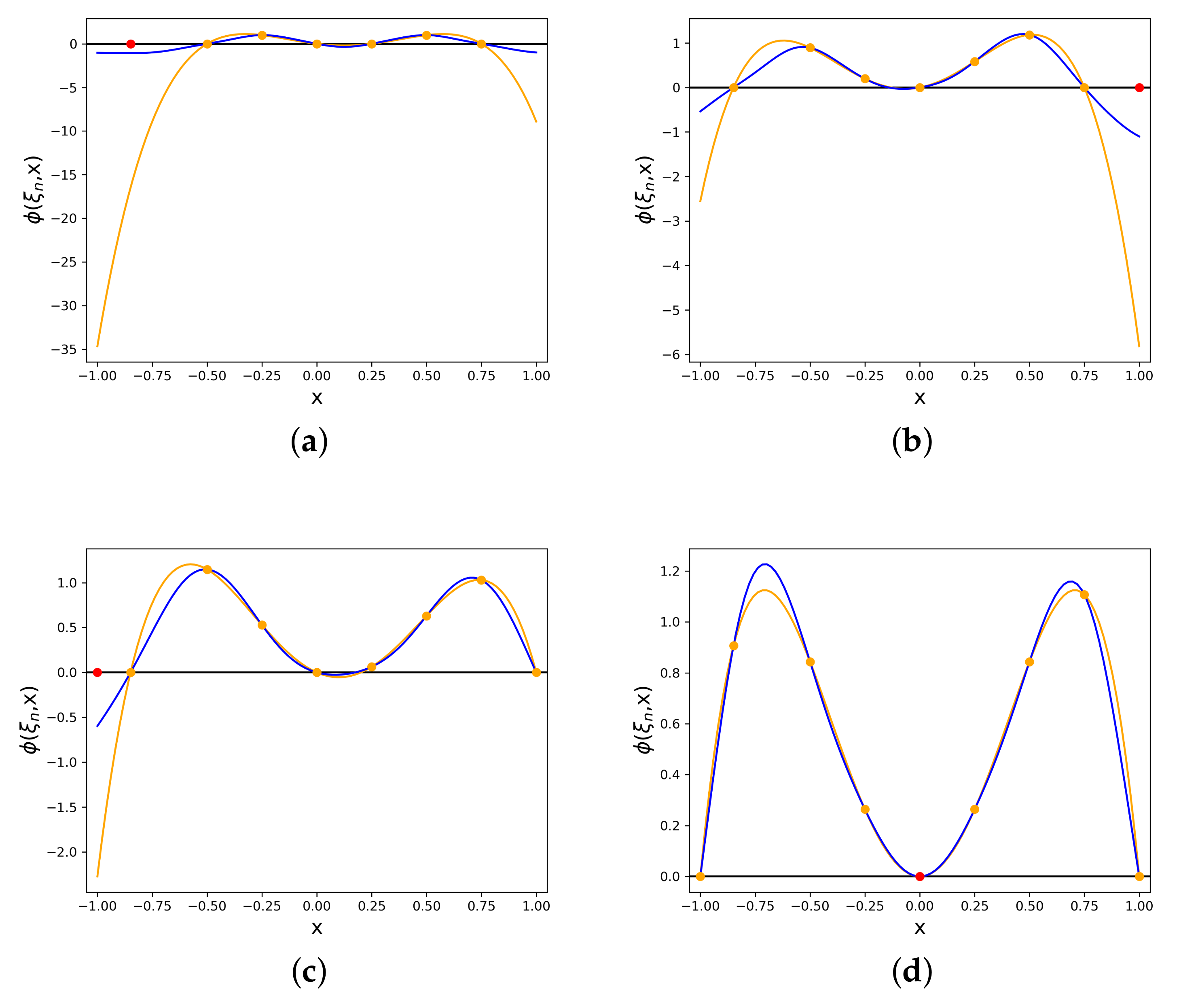
In Figure 2, the adaptive point acquisition in the first 4 iterations of the ADA-GPR for a mathematical toy example $f(x,\theta )={\theta }_2{x}^2+{\theta }_{1}x+\theta$ is illustrated. We can observe how the algorithm selects the next candidate point $x_{n+1}$ in these illustrations. We note that the point selected via the acquisition function can differ from the point we select via the exact values of ${\varphi }_D$.

To end this section, we discuss the quality of the design we obtain with the novel algorithm. For the YBT algorithm as well as the VDM, it is shown in [1,22] that the objective values converge to the optimal objective value with increasing number of iterations. We also have a stopping criterion that gives an error bound on the computed design. We refer to [1] for details. As we are using an approximation in the ADA-GPR, we cannot derive such results. The maximum error in our approximation will always present a bound for the error in the objective values of the design. However, we highlight once more that the aim of the ADA-GPR is to efficiently compute an approximation of an optimal design—where efficiency refers to less evaluations of the Jacobian matrix $D_{\theta }f\left(x\right)$. For models that we cannot evaluate on a fine grid in the design space the ADA-GPR then presents a viable option to obtain designs in the continuous design space X.

4. Results

We now provide two examples from chemical engineering to illustrate the performance of the new ADA-GPR (Section 3) compared to known the VDM and YBT algorithm (both Section 2.1). In this section we compute optimal designs with respect to the log-D-Criterion. The corresponding optimization problem (Problem (11)) we solve with each algorithm is given by

$${\xi }^{*}=arg\underset{\xi \in \Xi \left(X\right)}{max}lo{g}_{10}\left(det\left(M\left(\xi \right)\right)\right).$$

(25)

In our examples, the design space X is given as a range in $R^{d_X}$. The resulting bounds on x are given in each example specifically.

We then compare the results and the runtimes of the different methods. The models we present in this section are evaluated in CHEMASIM and CHEMADIS, the BASF inhouse simulators (Version 6.6 [36] BASF SE, Ludwigshafen, Germany), using the standard settings.

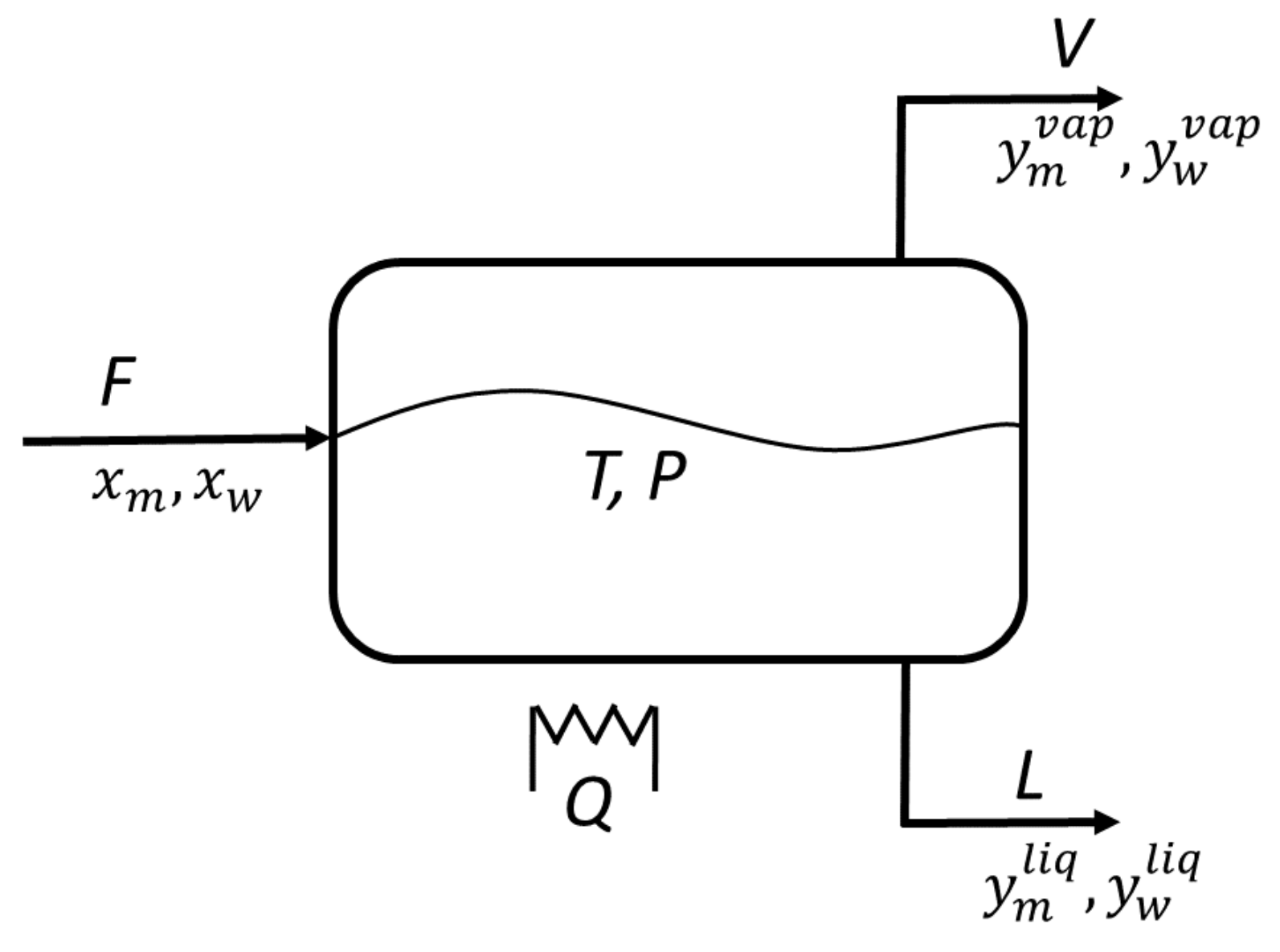
The first example we consider is a flash. A liquid mixture consisting of two components enters the flash, where the mixture is heated and partially evaporates. One obtains an vapor liquid equilibrium at temperature T and pressure P. In Figure 3, the flash unit with input and output streams is sketched. The relations in the flash unit are governed by the MESH equations (see Appendix A and [37]).

Initially, we consider a mixture composed of methanol and water and compute optimal designs for this input feed. In the second step, we replace the water component with acetone and repeat the computations. The model, and in particular, the MESH equations remain the same, however, parameters of the replaced component can vary. Details on the parameters for vapor pressure are given in the Appendix A.

In the following, we denote the molar concentrations of the input stream by $x_m$ and $x_w$, those of the liquid output stream by $y_m^{liq}$ and $y_w^{liq}$ and those of the vapor output stream by $y_m^{vap}$ and $y_w^{vap}$. Additionally, we introduce the molar flow rates F of the input stream, V of the vapor output stream and L of the liquid output stream.

We consider the following design of experiments setup:

• two inputs, P and $x_m$. Here P denotes the pressure in the flash unit that ranges from 0.5–5 bar. The variable $x_m$ gives the molar concentration of methanol in the liquid input stream. This concentration is between 0 and 1 ^{$\mathrm{mol}$}/_{$\mathrm{mol}$}.
• two outputs, T and $y_m^{vap}$. The temperature in degree Celsius at equilibrium T is measured as well as the molar concentration $y_m^{vap}$ ^{$\mathrm{mol}$}/_{$\mathrm{mol}$} of the evaporated methanol at equilibrium.
• four model parameters $a_{12},a_{21},b_{12}$ and $b_{21}$. These are parameters of the activity coefficients ${\gamma }_w$ and ${\gamma }_m$ in the MESH equations (Appendix A)—the so-called non-random two-liquid (NRTL) parameters.

We fix the flow rates $F=1$ ^{$\mathrm{kmol}$}/h and $V={10}^{-6}$ ^{$\mathrm{kmol}$}/h. Given the inputs P and $x_m$ we can then solve the system of equations to obtain the values of T and $y_m^{vap}$. We represent this via the model function f as

$$\left(\begin{array}{c}{y}_m^{vap}\\ T\end{array}\right)=f\left({\left(x_m,P\right)}^T,{\left(a_{12},a_{21},b_{12},b_{21}\right)}^T\right),$$

(26)

with $f:\left([0,1]\times [0.5,5]\right)\times {\mathbb{R}}^4\to {\mathbb{R}}^2$.

For the VDM and the YBT algorithm we need to replace the continuous design space with a grid. Therefore, we set

$$X_{grid}=\left\{\left.\left(\frac{i}{100}\frac{\mathrm{mol}}{\mathrm{mol}},\frac{10+j}{20}\mathrm{bar}\right)\right|i=0,\dots ,100,j=0,\dots ,90\right\}.$$

(27)

This set corresponds to a grid with 9191 design points.

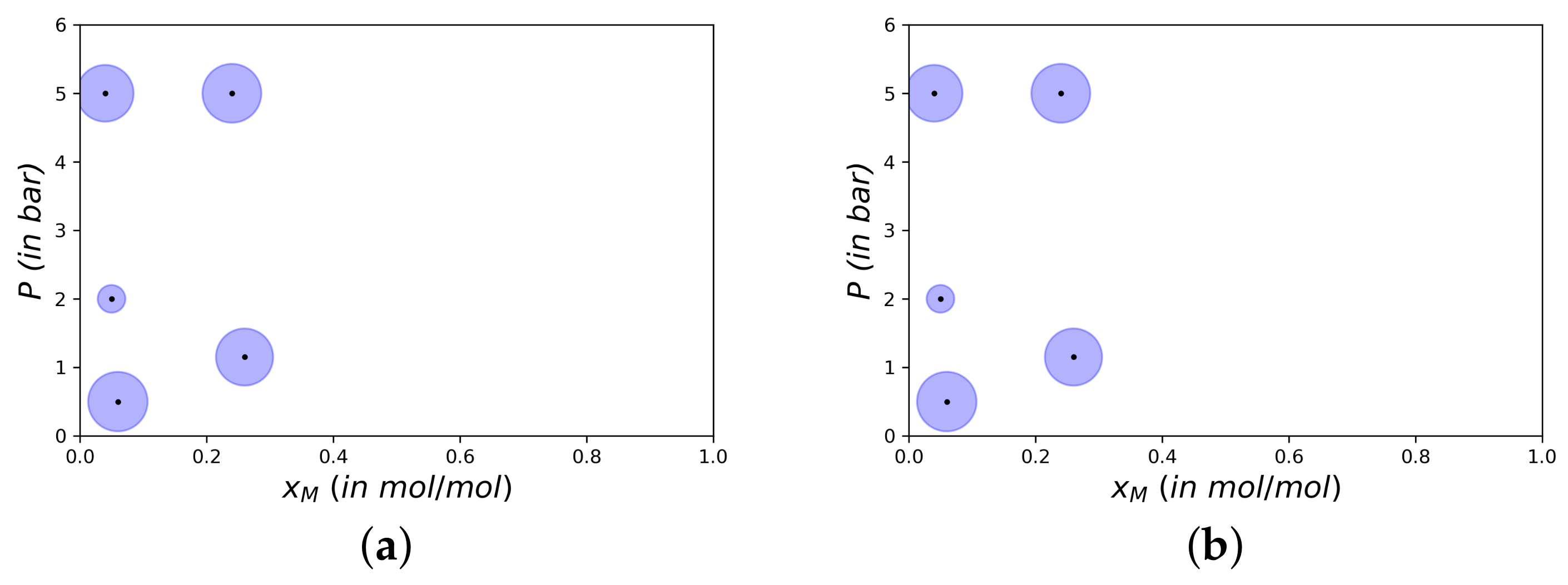
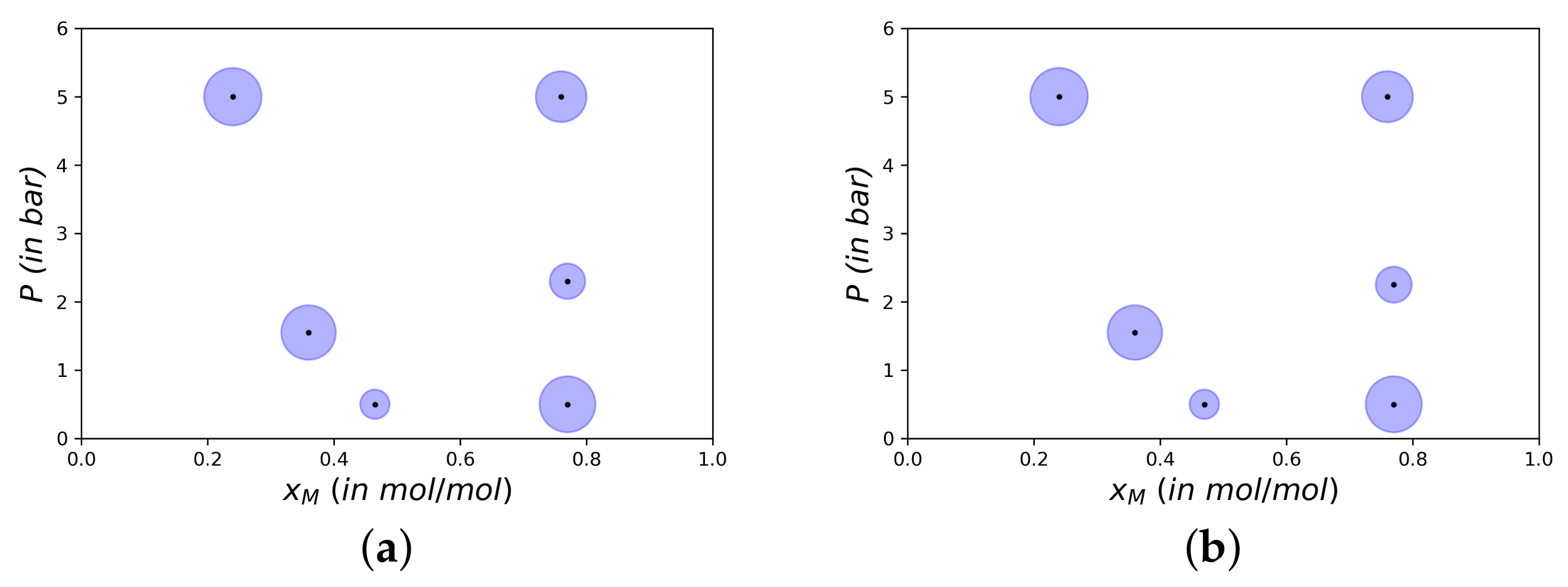
The designs ${\xi }_{VDM}$ and ${\xi }_{YBT}$ which the VDM and YBT algorithm compute for a flash with methanol–water input feed are given in

Table 1. Optimal design ${\xi }_{VDM}$ computed with the vertex direction method (VDM) for the flash with a methanol-water input feed.

	${\mathit{x}}_{\mathit{M}}$	P	Weight
1	0.06 $\mathrm{mol}$/$\mathrm{mol}$	0.50 bar	0.2477
2	0.05 $\mathrm{mol}$/$\mathrm{mol}$	2.00 bar	0.0538
3	0.04 $\mathrm{mol}$/$\mathrm{mol}$	5.00 bar	0.2258
4	0.24 $\mathrm{mol}$/$\mathrm{mol}$	5.00 bar	0.2426
5	0.26 $\mathrm{mol}$/$\mathrm{mol}$	1.15 bar	0.2287

and

Table 2. Optimal design ${\xi }_{YBT}$ computed with the YBT algorithm for the flash with a methanol-water input feed.

	${\mathit{x}}_{\mathit{M}}$	P	Weight
1	0.04 $\mathrm{mol}$/$\mathrm{mol}$	5.00 bar	0.2259
2	0.06 $\mathrm{mol}$/$\mathrm{mol}$	0.50 bar	0.2480
3	0.05 $\mathrm{mol}$/$\mathrm{mol}$	2.00 bar	0.0539
4	0.24 $\mathrm{mol}$/$\mathrm{mol}$	5.00 bar	0.2430
5	0.26 $\mathrm{mol}$/$\mathrm{mol}$	1.15 bar	0.2292

and in Figure 4. We note that only design points with a weight larger than 0.001 are given—in particular for the VDM, where the weights of the initial points only slowly converge to 0.

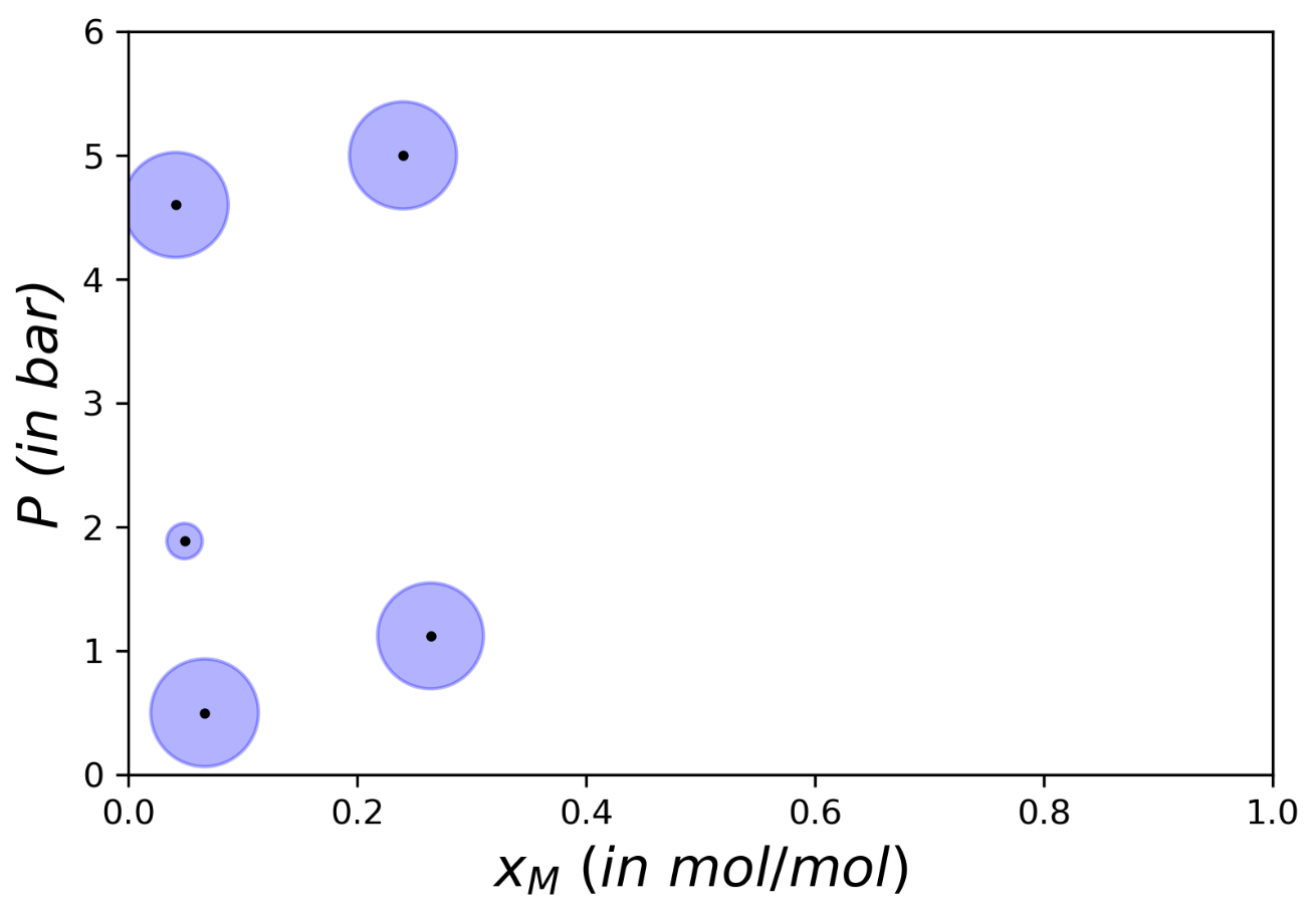
The ADA-GPR, on the other hand, is initialized with 50 starting candidate points. We obtain the design ${\xi }_{ADAGPR}$ given in

Table 3. Optimal designs ${\xi }_{ADAGPR}$ computed with the ADA-GPR for the flash with a methanol-water input feed.

	${\mathit{x}}_{\mathit{M}}$	P	Weight
1	0.0667 $\mathrm{mol}$/$\mathrm{mol}$	0.5000 bar	0.2487
2	0.0415 $\mathrm{mol}$/$\mathrm{mol}$	4.6000 bar	0.2367
3	0.2642 $\mathrm{mol}$/$\mathrm{mol}$	1.1209 bar	0.2402
4	0.2401 $\mathrm{mol}$/$\mathrm{mol}$	5.0000 bar	0.2464
5	0.0492 $\mathrm{mol}$/$\mathrm{mol}$	1.8857 bar	0.0271

and in Figure 5. Here, we also only give points with a weight larger than 0.001. Additionally, we have clustered some of the design points. We refer to Section 6 for details on the clustering.

In

Table 4. Objective values, runtime and number of iterations of all three algorithms for the flash with a methanol-water input feed.

	VDM	YBT Algorithm	ADA-GPR
Objective value	7.9327	7.9334	7.9124
Iterations	10,000	10	136
Evaluations of the Jacobian	9191	9191	151
Runtime	4241.88 s	1790.21 s	124.10 s

the objective value, the total runtime, the number of iterations and the number of evaluated Jacobian matrices $Df$ is listed. We recall, that we aim at maximizing the objective value in Optimization Problem (25) and a larger objective value is therefore more favorable. A detailed breakdown of the runtime is given in

Table 5. Detailed breakdown of the runtime of all algorithms for the flash with a methanol-water input feed.

Runtime	VDM	YBT Algorithm	ADA-GPR
Total	4241.88 s	1790.21 s	124.10 s
Jacobian evaluation	1787.22 s	1787.22 s	25.20 s
Optimization: weights	-	0.34 s	4.41 s
Optimization: acquisition function	2447.71 s	2.52 s	46.44 s
Optimization: hyperparameters	-	-	43.01 s

. Here, we differentiate between the time contributed to evaluations of the Jacobians $D_{\theta }f$, the optimization of the weights $w_i$, the optimization of the hyperparameters $\sigma$ of the GPR and the optimization of the point acquisition function.

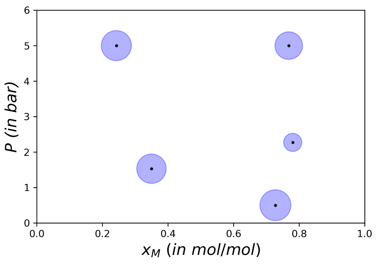
Next, we replace the mixture of water and methanol by a new mixture consisting of methanol and acetone. The designs ${\xi }_{VDM},{\xi }_{YBT}$ and ${\xi }_{ADAGPR}$—computed by the VDM, YBT algorithm and the ADA-GPR respectively—are given in

Table 6. Optimal design ${\xi }_{VDM}$ computed with the vertex direction method (VDM) for the flash with a methanol–acetone input feed.

	${\mathit{x}}_{\mathit{M}}$	P	Weight
1	0.76 $\mathrm{mol}$/$\mathrm{mol}$	5.00 bar	0.1816
2	0.24 $\mathrm{mol}$/$\mathrm{mol}$	5.00 bar	0.2324
3	0.36 $\mathrm{mol}$/$\mathrm{mol}$	1.55 bar	0.2092
4	0.77 $\mathrm{mol}$/$\mathrm{mol}$	0.50 bar	0.2199
5	0.47 $\mathrm{mol}$/$\mathrm{mol}$	0.50 bar	0.0605
6	0.77 $\mathrm{mol}$/$\mathrm{mol}$	2.30 bar	0.0887

,

Table 7. Optimal design ${\xi }_{YBT}$ computed with the YBT algorithm for the flash with a methanol–acetone input feed.

	${\mathit{x}}_{\mathit{M}}$	P	Weight
1	0.24 $\mathrm{mol}$/$\mathrm{mol}$	5.00 bar	0.2328
2	0.77 $\mathrm{mol}$/$\mathrm{mol}$	0.50 bar	0.2210
3	0.47 $\mathrm{mol}$/$\mathrm{mol}$	0.50 bar	0.0613
4	0.36 $\mathrm{mol}$/$\mathrm{mol}$	1.55 bar	0.2096
5	0.76 $\mathrm{mol}$/$\mathrm{mol}$	5.00 bar	0.1831
6	0.77 $\mathrm{mol}$/$\mathrm{mol}$	2.25 bar	0.0914

and

Table 8. Optimal design ${\xi }_{ADAGPR}$ computed with the ADA-GPR for the flash with a methanol–acetone input feed.

	${\mathit{x}}_{\mathit{M}}$	P	Weight
1	0.7277 $\mathrm{mol}$/$\mathrm{mol}$	0.5000 bar	0.2499
2	0.7684 $\mathrm{mol}$/$\mathrm{mol}$	5.0000 bar	0.1982
3	0.2428 $\mathrm{mol}$/$\mathrm{mol}$	5.0000 bar	0.2369
4	0.3498 $\mathrm{mol}$/$\mathrm{mol}$	1.5298 bar	0.2259
5	0.7805 $\mathrm{mol}$/$\mathrm{mol}$	2.2716 bar	0.0860

as well as in Figure 6 and Figure 7. We initialize the algorithms with the same number of points as for the water-methanol mixture. A detailed breakdown of the objective values, number of iterations and the runtime is given in

Table 9. Objective values, runtime and number of iterations of all three algorithms for the flash with a methanol-acetone input feed.

	VDM	YBT Algorithm	ADA-GPR
Objective value	18.5060	18.5064	18.5020
Iterations	10,000	16	58
Evaluations of the Jacobian	9191	9191	77
Runtime	4287.86 s	1840.21 s	56.17 s

and

Table 10. Detailed breakdown of the runtime of all algorithms for the flash with a methanol–acetone input feed.

Runtime	VDM	YBT Algorithm	ADA-GPR
Total	4287.86 s	1840.21 s	56.17 s
Jacobian evaluation	1835.99 s	1835.99 s	13.69 s
Optimization: weights	-	0.18 s	0.80 s
Optimization: acquisition function	2443.89 s	3.86 s	16.55 s
Optimization: hyperparameters	-	-	24.08 s

.

The second example we consider is the fermentation of baker’s yeast. This model is taken from [8,13], where a description of the model is given and OED results for uncertain model parameters $\theta$ are presented.

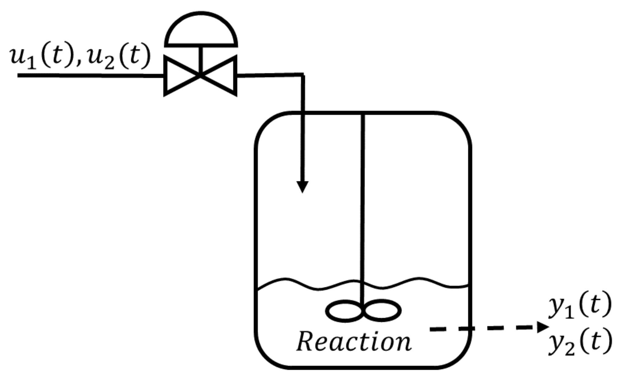
Yeast and a substrate are put into a reactor and the yeast ferments. Thus the substrate concentration $y_2$ decreases over time, while the biomass concentration $y_1$ increases. During this process we add additional substrate into the reactor via an input feed. This feed is governed by two (time-dependent) controls $u_1$ and $u_2$. Here, $u_1$ denotes the dilution factor while $u_2$ denotes the substrate concentration of the input feed. A depiction of the setup is given in Figure 8.

Mathematically, the reaction is governed by the system of equations

$$\begin{array}{cc}\hfill \frac{d{y}_1\left(t\right)}{dt}& =(r\left(t\right)-u_1\left(t\right)-{\theta }_4)·y_1\left(t\right)\hfill \\ \hfill \frac{d{y}_2\left(t\right)}{dt}& =-\frac{r\left(t\right)·u_1\left(t\right)}{{\theta }_3}+u_1\left(t\right)·\left(u_2\left(t\right)-y_2\left(t\right)\right)\hfill \\ \hfill r\left(t\right)& =\frac{{\theta }_1·y_2\left(t\right)}{{\theta }_2+y_2\left(t\right)}.\hfill \end{array}$$

(28)

The time t is given in hours h. We solve the differential equations inside the CHEMADIS Software by a 4th order Runge-Kutta method with end time $t_{end}=20\mathrm{h}$.

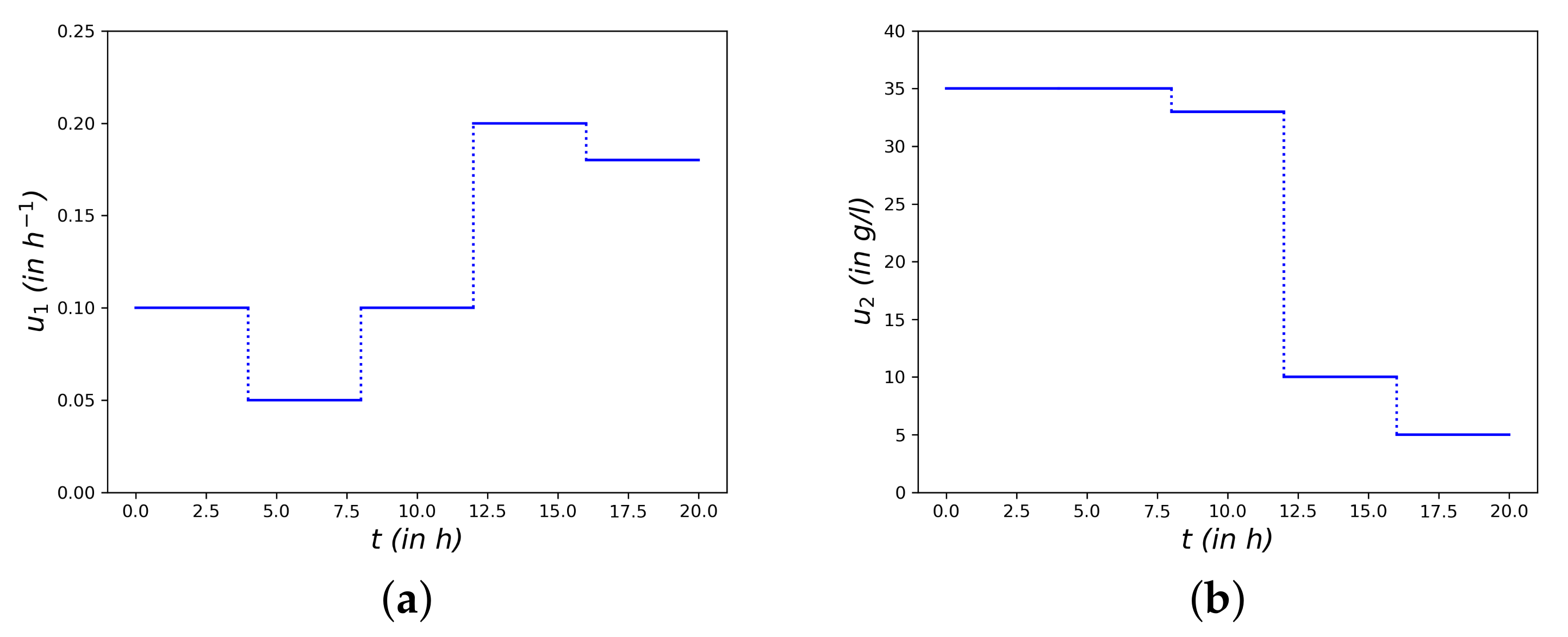
In order to obtain a design of experiments setup we parameterize the dynamical system and replace the time-dependent functions by time-independent parameters. As inputs, we consider the functions $u_1\left(t\right),u_2\left(t\right)$ and the initial biomass concentration $y_1^0=y_1\left(0\right)$. The functions $u_i$ with $i=1,2$ are modeled as step functions with values $u_i\left(t\right)=u_{ij}$ for $t\in \left[4j,(4+1)j\right]h$, where $j=0,\dots ,4$. This results in a 11-dimensional design space with design points

$$x={\left(y_1^0,u_{10},\dots ,u_{14},u_{20},\dots ,u_{24}\right)}^T.$$

(29)

We bound the initial biomass concentration $y_1^0$ by 1 g/L and 10 g/L, the dilution factor $u_{1j}$ by the range 0.05–0.2 h⁻¹ and the substrate concentration of the feed $u_{2j}$ by 5–35 g/L. In Figure 9, an example of the parameterized functions $u_1$ and $u_2$ is plotted.

As outputs, we take measurements of the biomass concentration $y_1$ in g/L and the substrate concentration $y_2$ in g/L. These measurements are taken at the 10 time points $t_j^y=2j+2h$ for $j=0,\dots ,9$, each. Thus we obtain a 20-dimensional output vector

$$y={\left(y_1\left(t_0^y\right),\dots ,y_1\left(t_9^y\right),y_2\left(t_0^y\right),\dots ,y_2\left(t_9^y\right)\right)}^T.$$

(30)

The model parameters are ${\theta }_1-{\theta }_4$, for which we insert our current best estimate ${\theta }_i=0.5$ for $i=1,\dots ,4$. This leaves one degree of freedom in the model, the initial substrate concentration, which we set as $y_2\left(0\right)=0.1$ g/L.

For the VDM and the YBT algorithm we introduce the grid consisting of 15,552 design points. As the design space X has 11 dimensions this grid is very coarse, despite the large amount of points. The designs ${\xi }_{VDM}$ and ${\xi }_{YBT}$ computed with the VDM and YBT algorithm are given in

Table 11. Optimal design ${\xi }_{VDM}$ computed with the VDM for the yeast fermentation.

	${\mathit{y}}_1^0$	${\mathit{u}}_{10}$	${\mathit{u}}_{11}$	${\mathit{u}}_{12}$	${\mathit{u}}_{13}$	${\mathit{u}}_{14}$	${\mathit{u}}_{20}$	${\mathit{u}}_{21}$	${\mathit{u}}_{22}$	${\mathit{u}}_{23}$	${\mathit{u}}_{24}$	Weight
1	10 g/L	0.05 h−1	0.05 h−1	0.05 h−1	0.05 h−1	0.05 h−1	5 g/L	35 g/L	35 g/L	35 g/L	5 g/L	0.2445
2	10 g/L	0.2 h−1	0.05 h−1	0.05 h−1	0.05 h−1	0.05 h−1	20 g/L	20 g/L	20 g/L	20 g/L	5 g/L	0.1111
3	10 g/L	0.2 h−1	0.05 h−1	0.05 h−1	0.05 h−1	0.05 h−1	35 g/L	35 g/L	35 g/L	35 g/L	5 g/L	0.4517
4	10 g/L	0.2 h−1	0.05 h−1	0.05 h−1	0.05 h−1	0.05 h−1	35 g/L	5 g/L	35 g/L	20 g/L	5 g/L	0.1920

and

Table 12. Optimal design ${\xi }_{YBT}$ computed with the YBT algorithm for the yeast fermentation.

	${\mathit{y}}_1^0$	${\mathit{u}}_{10}$	${\mathit{u}}_{11}$	${\mathit{u}}_{12}$	${\mathit{u}}_{13}$	${\mathit{u}}_{14}$	${\mathit{u}}_{20}$	${\mathit{u}}_{21}$	${\mathit{u}}_{22}$	${\mathit{u}}_{23}$	${\mathit{u}}_{24}$	Weight
1	10 g/L	0.05 h−1	0.05 h−1	0.05 h−1	0.05 h−1	0.05 h−1	5 g/L	35 g/L	35 g/L	35 g/L	5 g/L	0.2446
2	10 g/L	0.2 h−1	0.05 h−1	0.05 h−1	0.05 h−1	0.05 h−1	20 g/L	20 g/L	20 g/L	20 g/L	5 g/L	0.1113
3	10 g/L	0.2 h−1	0.05 h−1	0.05 h−1	0.05 h−1	0.05 h−1	35 g/L	35 g/L	35 g/L	35 g/L	5 g/L	0.4520
4	10 g/L	0.2 h−1	0.05 h−1	0.05 h−1	0.05 h−1	0.05 h−1	35 g/L	5 g/L	35 g/L	20 g/L	5 g/L	0.1921

. The ADA-GPR is initiated with 200 design points. The computed design ${\xi }_{ADAGPR}$ is given in

Table 13. Optimal design ${\xi }_{ADAGPR}$ computed with the novel ADA-GPR for the yeast fermentation.

	${\mathit{y}}_1^0$	${\mathit{u}}_{10}$	${\mathit{u}}_{11}$	${\mathit{u}}_{12}$	${\mathit{u}}_{13}$	${\mathit{u}}_{14}$	${\mathit{u}}_{20}$	${\mathit{u}}_{21}$	${\mathit{u}}_{22}$	${\mathit{u}}_{23}$	${\mathit{u}}_{24}$	Weight
1	10 g/L	0.1805 h−1	0.05 h−1	0.05 h−1	0.05 h−1	0.05 h−1	35 g/L	35 g/L	35 g/L	35 g/L	5 g/L	0.3594
2	10 g/L	0.05 h−1	0.1031 h−1	0.05 h−1	0.05 h−1	0.05 h−1	5 g/L	35 g/L	35 g/L	35 g/L	5 g/L	0.2543
3	7.7720 g/L	0.2 h−1	0.1227 h−1	0.05 h−1	0.05 h−1	0.05 h−1	35 g/L	35 g/L	35 g/L	23.9587 g/L	5 g/L	0.3860

. Again we do not list points with a weight smaller than 0.001 and perform the clustering described in Section 6 for the ADA-GPR. As for the flash, we also give a detailed breakdown of the objective value, number of iterations and the runtime in

Table 14. Objective values, runtime and number of iterations of all three algorithms for the yeast fermentation.

	VDM	YBT Algorithm	ADA-GPR
Objective value (maximization)	8.0332	8.0339	8.7029
Iterations	10,000	5	261
Evaluations of the Jacobian	15,552	15,552	409
Runtime	115,265.53 s	111,108.58 s	4939.24 s

and

Table 15. Detailed breakdown of the runtime of all algorithms for the yeast fermentation.

Runtime	VDM	YBT Algorithm	ADA-GPR
Total	115,265.53 s	111,108.58 s	4939.24 s
Jacobian evaluation	111,106.29 s	111,106.29 s	2851.94 s
Optimization: weights	-	0.10 s	7.98 s
Optimization: acquisition function	4151.50 s	2.11 s	392.89 s
Optimization: hyperparameters	-	-	1660.15 s

.

$$X_{grid}=\{1{}^{\mathrm{g}}/{}_{\mathrm{L}},10{}^{\mathrm{g}}/{}_{\mathrm{L}}\}\times {\{0.05{\mathrm{h}}^{-1},0.2{\mathrm{h}}^{-1}\}}^5\times {\{5{}^{\mathrm{g}}/{}_{\mathrm{L}},20{}^{\mathrm{g}}/{}_{\mathrm{L}},35{}^{\mathrm{g}}/{}_{\mathrm{L}}\}}^5$$

(31)

5. Discussion

In this section, we discuss the numerical results presented in Section 4. Both examples presented differ greatly in complexity and input dimension and are discussed separately.

For the flash we observe that the ADA-GPR can compute near optimal designs in significantly less time than the state-of-the-art YBT algorithm. In particular, we need less evaluations of the Jacobian $D_{\theta }f$ and can drastically reduce the time required for these evaluations. This is due to the fact, that the ADA-GPR operates on the continuous design space and uses an adaptive sampling instead of a pre-computed fine grid. The time reduction is also noticeable in the total runtime. Despite requiring additional steps—like the optimization of the hyperparameters of the GPR—as well as requiring more iterations before the algorithm terminates, the ADA-GPR is faster than the YBT algorithm. The runtime needed is reduced by a factor greater than 10.

We observe that the VDM and the YBT algorithm compute designs with a larger objective value. This occurs as we use an approximation in the ADA-GPR instead of the exact function values $\varphi (\xi ,x)$. Therefore we expect to have small errors in our computations. In particular for low dimensional design spaces—where the sampling of a fine grid is possible—we expect the grid based methods to result in better objective values. However, from a practical point of view this difference is expected to be negligible.

For the yeast fermentation we make a similar observation. The ADA-GPR can significantly reduce the number of evaluations of the Jacobian $D_{\theta }f$ as well as the runtime. In contrast to the flash distillation, ADA-GPR also computes a design with a larger—and thereby considerably better—objective value than the VDM and the YBT algorithm.

As the design space is 11-dimensional, the grid $X_{grid}$ consisting of 15,552 design points is still very coarse. The computation of the Jacobians $D_{\theta }f$ for these points takes a long time—more than 30 h. As we have a coarse grid, we do not expect the designs to be optimal on the continuous design space. In comparison, the ADA-GPR operates on the continuous design space and selects the next candidate points based on the existing information. We see that the adaptive sampling in the continuous space leads to a better candidate point set than the (coarse) grid approach. Using a finer grid for the VDM and the YBT algorithm is however not possible, as the computations simply take too long.

We conclude that the ADA-GPR outperforms the state-of-the-art YBT algorithm for models with high-dimensional design spaces—where sampling on a fine grid is computationally not tractable. Additionally, the ADA-GPR computes near optimal designs for models with low-dimensional design spaces in less time. The algorithm is particular useful for dynamical models, where a parameterization of the dynamic components can lead to many new design variables. We hereby make use of an adaptive point selection based on information from the current candidate points instead of selecting an arbitrary fixed grid.

The new algorithm also leaves room for improvement. In Table 5, Table 10 and Table 15 we see that we can reduce the runtime contributed to the evaluations of the Jacobian. The runtimes for the optimization of the acquisition function as well as the optimization of the hyperparameters may increase compared to the YBT algorithm. Here, more advanced schemes for estimating the hyperparameters can be helpful.

Further room for improvement of the ADA-GPR is the stopping criterion and the resulting precision of the solution. Both VDM and YBT algorithm have a stopping criterion which gives an error bound on the objective value, see [1]. For the ADA-GPR we have no such criterion and instead use a heuristic termination criterion—see Section 6 for a detailed description. A more rigorous stopping criterion is left for future research.

6. Materials and Methods

In this section, we present details on our implementations of the VDM, the YBT algorithm and the ADA-GPR, which are introduced in Section 2.1 and Section 3. We implemented all methods using python [38]. The models f were evaluated using CHEMASIM and CHEMADIS, the BASF inhouse simulators (Version 6.6 [36] BASF SE, Ludwigshafen, Germany).

We begin by describing the grid-based VDM and YBT algorithm. For both methods, we take a grid $X_{grid}$ as input consisting of at least $d_{\Theta }+1$ design points, where $d_{\Theta }$ denotes the number of unknown parameters $\theta$. We select a random initial set of candidate points $X_{n_0}$ consisting of $n_0=d_{\Theta }+1$ grid points $x_i\in X_{grid}$. This amount of points is suggested in [22], a larger amount is possible as well and can increase the numeric stability.

In the VDM, we assign each candidate points $x_1,\dots ,x_{n_0}$ the weight $w_i=\frac{1}{n_0}$ in order to obtain the initial design ${\xi }_{n_0}$. In the YBT algorithm, we instead solve the optimal weights problem

$$\begin{array}{cc}\hfill \underset{w_i}{min}& \mathsf{\Phi }\left(\sum _{i=1}^{n_0}{w}_i·\mu \left(x_i\right)\right)\hfill \\ \hfill s.t.& \sum _{i=1}^{n_0}{w}_i=1,0\le w_i.\hfill \end{array}$$

(32)

We solve this problem by reformulating it as a SDP and use the MOSEK Software [39] (MOSEK ApS, Copenhagen, Denmark) to solve the SDP. We assign the optimal weights $w_i^{*}$ to the candidate points $x_i\in X_{n_0}$ to obtain the initial design ${\xi }_{n_0}$.

Should the Fisher information matrix $M\left({\xi }_{n_0}\right)$ of the initial design ${\xi }_{n_0}$ be singular, we discard the design and the candidate points $X_{n_0}$ and select a new set of random candidate points.

Next, we describe how we have implemented the iterative step of each algorithm. In order to obtain

$$x_{n+1}=arg\underset{x}{min}\varphi ({\xi }_n,x)$$

(33)

we evaluate the function $\varphi ({\xi }_n,x)$ for every grid point $x\in X_{grid}$. We then add $x_{n+1}$ to the set of candidate points $X_n$ and adjust the weights. For the VDM, we assign the new candidate point $x_{n+1}$ the weight $w_{n+1}=\frac{1}{n+1}$. The weights $w_i$ of all the previous candidate points are adjusted by multiplying with the factor $1-\frac{1}{n+1}$, resulting in the update

$$w_i\to w_i·\left(1-\frac{1}{n+1}\right).$$

(34)

This factor is chosen according to [1], Chapter 3.1.1. In the YBT algorithm we instead adjust the SDP to also account for the new candidate point $x_{n+1}$ and re-solve the weight optimization problem. With the updated weights we obtain the design ${\xi }_{n+1}$ and can iterate.

Last we discuss our stopping criterion. We set a value $\epsilon ={10}^{-3}$ and stop the algorithm as soon as $min\varphi ({\xi }_n,x)>-\epsilon$. The computed design ${\xi }_n$ then fulfills $\mathsf{\Phi }\left(M\left({\xi }_n\right)\right)-{min}_{\xi \in \Xi \left(X\right)}\mathsf{\Phi }\left(M\left(\xi \right)\right)<\epsilon$. Setting a smaller value of $\epsilon$ increases the precision of the design, but also increases the number of iterations needed. Additionally we terminate the algorithm if we reach 10,000 iterations.

Now we discuss our implementation of the novel ADA-GPR. As we want to use a Gaussian process regression, it is helpful to scale the inputs. We thus map the design space to the unit cube ${[0,1]}^{d_X}$.

In the ADA-GPR we select a number $n_0>d_{\Theta }$ of initial candidate points. For the examples from Section 4 we have selected 50 and 200 initial points respectively. The initial points are set as the first $n_0$ points of the $d_X$-dimensional Sobol-sequence [40,41]. This is a pseudo-random sequence which uniformly fills the unit cube ${[0,1]}^{d_X}$. In our experience, one has to set $n_0$ significantly larger than $d_{\Theta }$, on the one hand to ensure the initial Fisher information matrix is not singular, on the other hand to obtain a good initial approximation via the GPR. We obtain the weights for the candidate points $X_{n_0}$ analogously to the YBT Algorithm by solving the SDP formulation of the optimal weights problem with MOSEK.

Next, we compute a Gaussian process regression for the directional derivative $\varphi ({\xi }_n,x)$ based on the evaluations $\left(X_n,\varphi ({\xi }_n,X_n)\right)$. For this GPR, we use the machine learning library scikit–learn [42] with the squared exponential kernel—the radial basis function RBF. The kernel is dependent on 3 hyperparameters, a pre-factor ${\sigma }_f^2$, the length scale l and a regularity factor $\alpha$. The parameters ${\sigma }_f^2$ and l are chosen via the scikit-learn built-in loss function. They are chosen every time we fit the Gaussian process to the data, i.e., in every iteration. For the factor $\alpha$, we use cross-validation combined with a grid search, where we consider the 21 values $\alpha ={10}^{-10},{10}^{-9.5},{10}^{-9},\dots ,{10}^0$. As the cross-validation of the hyperparameters can be time-expensive, we do not perform this step in every iteration. Instead, we adjust $\alpha$ in the initial 10 iterations and then only every 10th iteration afterwards.

Now we discuss the optimization of the acquisition function

$$\mathrm{E}\left[\varphi ({\xi }_n,x)\left|X_n,\varphi ({\xi }_n,X_n)\right.\right]-\mathrm{Var}\left[\varphi ({\xi }_n,x)\left|X_n,\varphi ({\xi }_n,X_n)\right.\right].$$

(35)

In order to obtain a global optimum we perform a multistart, where we perform several optimization runs from different initial values. In our implementation we perform 10 optimization runs. The initial points are selected via the $d_X$-dimensional Sobol-sequence in the design space ${[0,1]}^{d_X}$. We recall, that the Sobol-sequence was also used to select the initial candidate points. In order to avoid re-using the same points, we store the index of the last Sobol-point we use. When selecting the next batch of Sobol-points, we take the points succeeding the stored index. Then, we increment the index. For the optimization we use the L-BFGS-B method from the scipy.optimize library [43,44].

Last, we present the stopping heuristic we use for the ADA-GPR. Throughout the iterations we track the development of the objective value and use the progress made as stopping criterion for the algorithm. For the initial 50 iterations, we do not stop the algorithm. After the initial iterations we consider the progress made over the last 40 percent of the total iterations. However we set a maximum of 50 iterations that we consider for the progress. For the current iteration $n_{cur}$, we thus compute $n_{stop}=max(0.6·n_{cur},n_{cur}-50)$ and consider the progress

$$\Delta {\mathsf{\Phi }}_{stop}=\mathsf{\Phi }\left(M\left({\xi }_{n_{cur}}\right)\right)-\mathsf{\Phi }\left(M\left({\xi }_{n_{stop}}\right)\right).$$

(36)

If $\Delta {\mathsf{\Phi }}_{stop}<0.001$, we stop the computation. Else, we continue with the next iteration.

For the tables and figures from Section 4 we have clustered the results from the ADA-GPR. Here we have proceeded as described in the following. We iterate through the support points of the computed design ${\xi }_{ADAGPR}$. Here we denote these support points by $s_i$. For each point $s_i$ we check if a second distinct point $s_j$ exists, such that $\parallel s_i-s_j\parallel <0.01$. If we find such a pair, we add these points to one joint cluster $C_i$. If we find a third point $s_k$ with either $\parallel s_k-s_j\parallel <0.01$ or $\parallel s_k-s_i\parallel <0.01$, the point $s_k$ is added to the cluster $C_i$ as well.

If for a point $s_i$ no point $s_j$ exists such that $\parallel s_i-s_j\parallel <0.01$, the point $s_i$ initiates its own cluster $C_i$.

After all points are divided into clusters, we represent each cluster $C_i$ by a single point $c_i$ with weight $w_i^c$. The point $c_i$ is selected as average over all points $s_j$ in the cluster $C_i$ via the formula

$$c_i=\frac{1}{|C_i|}\sum _{s_j\in C_i}{s}_j.$$

(37)

The weight $w_i^c$ is set as sum of the weights assigned to the points in the cluster $C_i$ and is computed via

$$w_i^c=\sum _{s_j\in C_i}{w}_j.$$

(38)

7. Conclusions

In this paper we have introduced a novel algorithm—the ADA-GPR—to efficiently compute locally optimal continuous designs. The algorithm uses an adaptive grid sampling method based on the Kiefer-Wolfowitz Equivalence Theorem. To avoid extensive evaluations of the Fisher information matrix, we approximate the directional derivative via a Gaussian process regression.

The ADA-GPR is particularly useful for models with high-dimensional design spaces, where traditional grid-based methods cannot be applied. Such models include dynamical systems, which need to be parameterized for the design of experiments setup. Additionally, optimal designs in low-dimensional spaces can also be computed efficiently by the ADA-GPR. In this paper, we have considered two examples from chemical engineering to verify these results.

In future work we want to further improve the ADA-GPR. For this purpose, we want to investigate the quality of the computed designs in order to have an indication on the optimal value. Another focus is the optimization of the acquisition function and the hyperparameters of the GPR, where we hope to improve the runtime even further. For this purpose we want to consider more advanced optimization and machine learning methods. Last, we want to extend the ADA-GPR to other design of experiment settings. These include incorporating existing experiments and considering robust designs instead of locally optimal ones.