Improved Continuous-Cycling Method for PID Autotuning

Abstract

An improved continuous-cycling method is proposed for the autotuning of the proportional–integral–derivative (PID) controller. The proposed method can identify the frequency response of the process at a preset phase angle without a modeling error. Moreover, it provides an exact frequency response even if a static disturbance is present. The proposed method is an improved version of the continuous-cycling method. The gain of the proportional controller in the continuous-cycling method is updated to obtain the continuous-cycling status automatically. To guarantee the preset phase angle of the frequency response, we place a phase shifter in the form of a time delay after the proportional controller. The results of simulation and experimental studies show that the proposed method can provide an exact frequency response even under static disturbance conditions and can be applied to real processes.

1. Introduction

Numerous modeling methods for proportional–integral–derivative (PID) autotuning have been developed since the original relay feedback method was proposed [1,2,3,4]. The original relay feedback method has limitations in that it shows modeling errors due to the harmonics of the relay signal and it is structurally impossible to assign a preset phase angle to the frequency response model. Moreover, it cannot manipulate the static disturbance in a systematic way, resulting in severe modeling errors or cycling failure.

Many researchers have tried to overcome the limitations of the original relay feedback method. Modified relay feedback methods using a six-level signal and a saturated relay signal were proposed to reduce the modeling error of the identified frequency response by reducing the harmonics [5,6]. Several relay feedback methods combined with an artificial time delay, a hysteresis, or a two-channel relay were developed to obtain the frequency response of the process corresponding to a preset phase angle [7,8,9,10,11,12]. Some relay feedback methods moved the reference value for switching the relay on/off to guarantee the same accuracy of the model even under static disturbance conditions [11,12,13,14,15,16]. Furthermore, an improved relay feedback method was developed to estimate the frequency response data of the process with better accuracy by removing the effects of measurement noises and disturbances [17] using a disturbance estimator and a noise magnitude estimator. All the previous relay feedback methods mentioned above are modifications of the relay feedback method. All of them still failed to completely remove the harmonics. Additionally, they have shortcomings in that the user must wait until the process converges to a steady state before conducting the relay test. Otherwise, the wrong deviation variables for the relay test are assigned and, as a result, a severely asymmetric limit cycle or cycling failure is obtained.

Low-order plus time-delay models have been identified from the relay feedback method [18,19,20,21,22]. The modeling methods using a curvature factor [18] and an input-biased relay [19] suffer from the effects of the harmonics, resulting in unavoidable modeling errors. The other methods based on an asymmetrical limit cycle [20] and a shape factor [21] have shortcomings in that they have to solve non-linear equations in an iterative manner. Moreover, all the methods [18,19,20,21,22] are inherently sensitive to plant–model structural mismatch and uncertainties such as disturbances and noises because the frequency information included in the limit cycle of the relay feedback test mainly concentrates on the zero and ultimate frequency.

Various process identification methods have been proposed to find high-order process models from closed-loop tests of relay feedback [12,23,24,25]. Even though the process identification methods and tuning methods based on multiple frequencies can provide better performances, they require heavier data processing and their implementations are more difficult compared to previous simple PID autotuning methods.

In this study, we propose an improved continuous-cycling method for the automatic tuning of the PID controller. The proportional gain of the proportional controller is automatically updated to obtain the continuous-cycling status. To guarantee the preset phase angle of the frequency response, we place a phase shifter in the form of a time delay after the proportional controller, as was done in [7] and [12]. The proposed method can identify the frequency response of the process at a preset phase angle without modeling error. It theoretically provides an exact frequency response even if a static disturbance is present or the initial status is not a steady state. Therefore, the user does not need to wait until the process converges to a steady state before conducting the proposed autotuning method. Furthermore, it is straightforward to obtain the exact first-order plus time-delay model without solving non-linear equations when there are no disturbances and the initial status is a steady state. We demonstrate numerically and experimentally that the proposed method can provide an exact frequency response even under static disturbance conditions, and can be applied to real processes.

2. Proposed Autotuning Method

Figure 1 and Figure 2 show a schematic diagram and a typical response for the proposed method. The proposed method is composed of a proportional controller, a continuous-cycler, and a phase shifter. The proportional gain of the proportional controller is automatically adjusted by the proposed continuous-cycler to derive the overall process to a continuous-cycling status.

Subsequently, the following characteristic equation for the continuous-cycling status is obtained.

$$1+k_c\mathrm{G}\left(i\omega \right)e^{ - i{\theta }_{ps}\omega }=0$$

(1)

Thus, the frequency response data of the process can be easily obtained as in Equation (2):

$$G\left(i\omega \right)= - e^{i{\theta }_{ps}\omega }/k_c$$

(2)

$$\angle G\left(i\omega \right)=-\pi +{\theta }_{ps}\omega =P{A}_{set}$$

(3)

$$\left|G\left(i\omega \right)\right|=1/k_c$$

(4)

$$G\left(0\right)=\overline{y}/\overline{u}, \overline{y}=\left(y_p+y_v\right)/2, \overline{u}=\left(u_p+u_v\right)/2$$

(5)

where $k_c$, $\omega ,$ and ${\theta }_{ps}$ denote the proportional gain, the frequency, and the time delay at the continuous-cycling status, respectively. $P{A}_{set}$ is a preset phase angle specified by the user. $G\left(0\right)$ is the frequency response of the zero frequency. $u_p$ and $y_p$ are the peak values of the process input and process output, respectively. $u_v$ and $y_v$ are the valley values of the process input and process output, respectively.

The phase shifter in Figure 1 plays a role in guaranteeing the preset phase angle of $P{A}_{set}$ by adjusting the time delay (${\theta }_{ps}$) every cycle according to Equation (3). As shown in Equation (4), the amplitude ratio of the frequency response data is $1/k_c$.

The proposed autotuning method with the continuous-cycler and the phase shifter goes through the following steps to obtain the continuous-cycling and the preset phase angle.

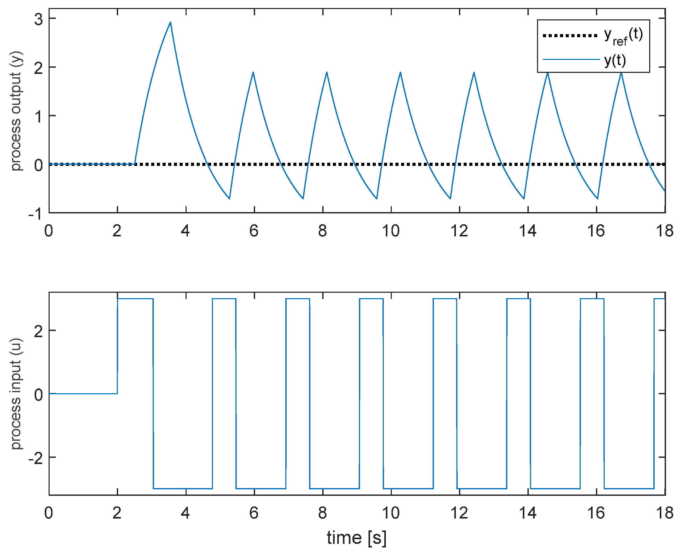
[Step 1.1] Set the lower and upper limits of the saturator, equivalently setting the limits of the control output for the sake of safety. Set the initial proportional gain ($k_c$) of the proportional controller to a very large value (e.g., 1000) to get the initial fully saturated cycle from 5 s to 14 s as in Figure 2. Set the preset phase angle ($P{A}_{set}$) of the frequency response data of the process and the setpoint of the proportional controller in accordance with the operator request. Run the proportional controller.

[Step 1.2] At the second peak of the process output, set the proportional gain ($k_c$) of the proportional controller to Equation (11) using the following equations:

$$a_1=\left(1-\cos \left(\omega T_{on}\right)\right)\left(u_{max}-u_{min}\right)/\pi$$

(6)

$$b_1=\sin \left(\omega T_{on}\right)\left(u_{max}-u_{min}\right)/\pi$$

(7)

$$u_{amplitude}=\sqrt{a_1^2+b_1^2}$$

(8)

$$y_{amplitude}=a/2$$

(9)

$$AI=\max \left(T_{on},T_{off}\right)/\min \left(T_{on},T_{off}\right)$$

(10)

$$k_{c,0}=1.6\times AI\times u_{amplitude}/y_{amplitude}$$

(11)

where $T_{on}$ and$T_{off}$ represent the time length corresponding to the lower and the upper saturation limits of the initial cycle, respectively, as shown in Figure 2. $\omega =2\pi /\left(T_{on}+T_{off}\right)$ is the frequency. $a_1$ and $b_1$ are the Fourier coefficients of the sine signal and the cosine signal of the fundamental frequency when the process input of the initial cycle is represented by the Fourier series. Then, $u_{amplitude}$ corresponds to the amplitude of process input ($u\left(t\right)$). $y_{amplitude}$ denotes the amplitude of the process output ($y\left(t\right)$) as shown in Figure 2. $AI$ is an index of asymmetry defined by Equation (10). $k_{c,0}$ is the initial value of the proportional gain for the next step.

$b_1=0$, $a_1=2\left(u_{max}-u_{min}\right)/\pi$, and $AI=1$ in the case that the process input is symmetric $(\mathrm{equivalently}, T_{on}=T_{off}$). Then, $k_{c,0}=1.6\times 2\times \left(u_{max}-u_{min}\right)/\left(\pi \times y_{amplitude}\right)$. $2\times \left(u_{max}-u_{min}\right)/\left(\pi \times y_{amplitude}\right)$ is the same as the ultimate gain obtained by the describing function analysis [12] from the symmetric relay feedback signals. Therefore, roughly speaking, the initial value $k_{c,0}$ is chosen by 1.6 times the ultimate gain. In the case that the process input is asymmetric, the initial value $k_{c,0}$ proportional to $AI$, as in Equation (11), is recommended to compensate for the phenomenon that $u_{amplitude}/y_{amplitude}$ decreases as $AI$ increases.

[Step 2.1] In the case of controller output saturation, decrease the proportional gain according to the proposed continuous-cycler as in Equation (13). The continuous-cycler would derive the cycling out of the saturation region automatically by decreasing the proportional gain.

$$T_{s,k}=max\left(T_{s,lower,k}, T_{s,upper,k}\right)$$

(12)

$$k_{c,k}=k_{c,k-1}(1-{\left(T_{s,k}/P_k\right)}^2), k=1,2,3,\cdots$$

(13)

where $T_{s,lower,k}$ and $T_{s,upper,k}$ are the time lengths corresponding to the lower and upper saturation limits of the k-th cycle, respectively, as shown in Figure 3. Lower and upper limit saturation mean that the process input is at the lower limit and the upper limit, respectively. Therefore, $T_{s,lower,k}$ and $T_{s,upper,k}$ are determined by measuring the time length that the process input is at the lower limit and the upper limit, respectively. $k_{c,k}$ is the proportional gain of the k-th cycle. $P_k$ is the period of the k-th cycle. In the case of controller output saturation, the proposed continuous-cycler in Equation (13) reduces the proportional gain in proportion to the square of the saturation portion within one period to derive the cycling out of the saturation.

[Step 2.2] In the case of no controller output saturation, the proposed continuous-cycler in Equation (14) decreases the proportional gain if the amplitude $\left(a_k\right)$ of the process output in the present cycle is greater than the amplitude $\left(a_{k-1}\right)$ of the process output in the previous cycle, as shown in Figure 4, and vice versa to derive the cycling into a continuous-cycling status automatically. $a_k$ and $a_{k-1}$ are obtained by measuring the difference between the valley value and the peak value of the process output.

$$k_{c,k}=k_{c,k-1}\left(\left(1-\alpha \right)+\alpha \left(a_{k-1}/a_k\right)\right)$$

(14)

Decreasing the constant $\alpha$ makes the convergence pattern of the proportional gain more stable but slower via less weighting on the ratio of the present and the previous peak values. The proportional gain does not change when the present peak and the previous peak are the same. $\alpha =0.3$ is recommended in this paper based on extensive simulation results.

[Step 3] Set the time delay as ${\theta }_k=\left(\pi +P{A}_{set}\right)/{\omega }_k$, ${\omega }_k=2\pi /P_k$ to guarantee the preset phase angle of $P{A}_{set}$.

[Step 4] Repeat [Steps 2–3] at each cycle until a continuous-cycling status is obtained.

[Step 5] Estimate the frequency response data of the process corresponding to the cycling frequency using Equation (2), and the frequency response corresponding to the zero frequency using Equation (5).

[Step 6.1] If you want to use only $G\left(i\omega \right)$ to tune the PID controller, calculate the tuning parameters of the PID controller using the ZN tuning rule or the gain-phase margin tuning rule [1,12].

[Step 6.2] If you want to use both $G\left(i\omega \right)$ and $G\left(0\right)$ to tune the PID controller, obtain the first-order plus time-delay model using the model reduction method [12] in Equations (15)–(17). In addition, calculate the tuning parameters of the PID controller using the IMC or ITAE tuning rules for the first-order plus time-delay model [12].

$$k=G\left(0\right)$$

(15)

$$\tau =\frac{\sqrt{k^2-{\left|G\left(i\omega \right)\right|}^2}}{\left|G\left(i\omega \right)\right|\omega }$$

(16)

$$\theta =\frac{-\angle G\left(i\omega \right)+arctan\left(-\tau \omega \right)}{\omega }$$

(17)

where $k$, $\tau$, and $\theta$ are the gain, time constant, and time delay of the first-order plus time-delay model.

The proposed autotuning method has remarkable advantages compared to previous relay feedback approaches. It guarantees the preset phase angle of the obtained frequency response data ($G\left(i\omega \right)$) of the process, as shown in Equation (3). Moreover, it theoretically provides exact frequency response data ($G\left(i\omega \right)$ and $G\left(0\right)$) of the process without any modeling errors because it uses a proportional controller to obtain the continuous-cycling status. The first-order plus time-delay model can be analytically obtained without solving non-linear equations, and the first-order plus time-delay model is also exact because it is based on exact frequency responses ($G\left(i\omega \right)$ and $G\left(0\right)$). Note that when the describing function analysis method is used to estimate the frequency response from the relay feedback test, the modeling error due to the harmonic terms of the relay feedback signal can be up to 5–18% for the first-order plus time-delay model even in ideal cases of no uncertainties and disturbances [22]. Furthermore, the proposed method still provides exact frequency response data $G\left(i\omega \right)$ of the process even under static disturbances or setpoint changes because static disturbances cannot affect the continuous-cycling. Meanwhile, static disturbances can severely distort the shape of the relay feedback signal, resulting in unacceptable modeling errors. Finally, changing the PID controller to the P controller of the proposed method is straightforward and simple. It is especially difficult to determine the deviation variables to apply the relay feedback method [1] if the initial state of the process is not a steady state. An incorrect definition of the deviation variables can severely distort the shape of the relay feedback signal, resulting in unacceptable modeling errors.

3. Simulation Study

Several processes were simulated to demonstrate the performance of the proposed autotuning method and compare it with the relay feedback method [1].

Figure 5, Figure 6, Figure 7 and Figure 8 show typical responses of the first-order plus time-delay process of $G\left(s\right)=exp\left(-\theta s\right)/\left(s+1\right)$ for the proposed autotuning method and the conventional relay feedback method [1]. A step input disturbance of 1.5 enters at the beginning of the autotuning methods in this case.

Table 1. Comparison of the proposed method and the relay feedback method [1] for the first-order plus time-delay process and $P{A}_{set}=-\pi$.

G(s)	$\frac{\mathit{e}\mathit{x}\mathit{p}\left(-\mathit{\theta }\mathit{s}\right)}{\left(\mathit{s}+1\right)}$
$\mathit{\theta }$	0.2			0.5			1.0
	Exact	Proposed	Relay	Exact	Proposed	Relay	Exact	Proposed	Relay
${\omega }_u$	8.44	8.44	5.81	3.67	3.67	2.90	2.03	2.03	1.77
$k_u$	8.50	8.50	3.50	3.81	3.81	3.19	2.26	2.26	2.01

and

Table 2. Comparison of the proposed method and the relay feedback method [1] combined with the time delay [7] for the first-order plus time-delay process and $P{A}_{set}=-3\pi /4$.

G(s)	$\frac{\mathit{e}\mathit{x}\mathit{p}\left(-\mathit{\theta }\mathit{s}\right)}{\left(\mathit{s}+1\right)}$
$\mathit{\theta }$	0.2			0.5			1.0
	Exact	Proposed	Relay	Exact	Proposed	Relay	Exact	Proposed	Relay
$\omega$	4.93	4.93	3.49	2.37	2.37	1.99	1.40	1.40	1.29
$\left|G\left(i\omega \right)\right|$	5.03	5.03	3.46	2.57	2.57	2.08	1.72	1.72	1.56

show the estimates of the proposed method and the relay feedback method [1]. As shown in Figure 5, Figure 6, Figure 7 and Figure 8, the proposed method successfully derives the process to a continuous-cycling status in a stable manner. In addition, the relay feedback method [1] shows significant modeling errors in estimating the frequency response data of the process. In contrast, our method provides the exact ultimate frequency (${\omega }_u$) and the ultimate gain ($k_u$) of the process for all the cases with various process parameters and static disturbances. While the proposed method shows remarkable advantages, the only shortcoming is that the convergence rate of the proposed method is slower, as much as about two or three cycles compared with that of the relay feedback method [1].

Figure 9, Figure 10, Figure 11 and Figure 12 and

Table 3. Estimates of the proposed method and the relay feedback method [1] for the high-order plus time-delay process and $P{A}_{set}=-\pi$.

G(s)	$\frac{\mathit{e}\mathit{x}\mathit{p}\left(-\mathit{\theta }\mathit{s}\right)}{{\left(\mathit{s}+1\right)}^5}$
$\mathit{\theta }$	0.0			0.1			0.3
	Exact	Proposed	Relay	Exact	Proposed	Relay	Exact	Proposed	Relay
${\omega }_u$	0.73	0.73	0.68	0.71	0.71	0.66	0.67	0.67	0.62
$k_u$	2.89	2.89	3.08	2.74	2.74	2.93	2.51	2.51	2.67

and

Table 4. Estimates of the proposed method and the relay feedback method [1] combined with the time delay [7] for the high-order plus time-delay process and $P{A}_{set}=-3\pi /4$.

G(s)	$\frac{\mathit{e}\mathit{x}\mathit{p}\left(-\mathit{\theta }\mathit{s}\right)}{{\left(\mathit{s}+1\right)}^5}$
$\mathit{\theta }$	0.0			0.1			0.3
	Exact	Proposed	Relay	Exact	Proposed	Relay	Exact	Proposed	Relay
$\omega$	0.51	0.51	0.48	0.50	0.50	0.47	0.47	0.47	0.45
$\left|G\left(i\omega \right)\right|$	1.78	1.78	1.82	1.74	1.74	1.77	1.66	1.66	1.70

show the typical responses of the high-order plus time-delay process of $G\left(s\right)=exp\left(-\theta s\right)/{\left(s+1\right)}^5$ and the estimates of the proposed method and the relay feedback method [1]. A step input disturbance of 2.0 enters at the beginning of the autotuning methods and the process output is contaminated by uniformly distributed random noise between −0.05 and +0.05. Hysteresis of 0.05 is used in finding the peak values of the process output in noisy environments. That is, it is concluded that the peak value is found if the present value is smaller than the previous maximum (peak candidate) values by as much as two times the hysteresis. The proposed method provides a stable convergence to a continuous-cycling status for the high-order plus time-delay process and an exact frequency response data of the process for all the cases, whereas the relay feedback method [1] cannot remove modeling errors due to the static disturbance in estimating the frequency response data.

Figure 13, Figure 14, Figure 15 and Figure 16 and

Table 5. Estimates of the proposed method and the relay feedback method [1] for the non-minimum phase process and $P{A}_{set}=-\pi$.

G(s)	$\frac{\mathit{e}\mathit{x}\mathit{p}\left(-\mathit{\theta }\mathit{s}\right)\left(-0.2\mathit{s}+1\right)}{{\left(\mathit{s}+1\right)}^3}$
$\mathit{\theta }$	0.0			0.1			0.3
	Exact	Proposed	Relay	Exact	Proposed	Relay	Exact	Proposed	Relay
${\omega }_u$	1.41	1.41	1.22	1.31	1.31	1.15	1.15	1.15	1.02
$k_u$	5.00	5.00	4.88	4.32	4.32	4.35	3.46	3.46	3.44

and

Table 6. Estimates of the proposed method and the relay feedback method [1] combined with the time delay [7] for the non-minimum phase process and $P{A}_{set}=-3\pi /4$.

G(s)	$\frac{\mathit{e}\mathit{x}\mathit{p}\left(-\mathit{\theta }\mathit{s}\right)\left(-0.2\mathit{s}+1\right)}{{\left(\mathit{s}+1\right)}^3}$
$\mathit{\theta }$	0.0			0.1			0.3
	Exact	Proposed	Relay	Exact	Proposed	Relay	Exact	Proposed	Relay
$\omega$	0.89	0.89	0.79	0.84	0.84	0.76	0.77	0.77	0.70
$\left|G\left(i\omega \right)\right|$	2.36	2.36	2.26	2.21	2.21	2.13	1.99	1.99	1.94

show the typical responses of the non-minimum phase process of $G\left(s\right)=exp\left(-\theta s\right)\left(-0.2s+1\right)/{\left(s+1\right)}^3$ and the estimates of the proposed method and the relay feedback method [1]. A step input disturbance of 2.0 enters at the beginning of the autotuning methods and the process output is contaminated by uniformly distributed random noise between −0.05 and +0.05. Hysteresis of 0.05 is used in finding the peak values of the process output in noisy environments. For all the cases, the proposed method provides a stable convergence to a continuous-cycling status for the non-minimum phase process and exact frequency response data of the process. The relay feedback method [1] suffers from modeling errors in estimating the frequency response data.

Figure 17, Figure 18, Figure 19 and Figure 20 and

Table 7. Estimates of the proposed method and the relay feedback method [1] for the integrating process and $P{A}_{set}=-\pi$.

G(s)	$\frac{\mathit{e}\mathit{x}\mathit{p}\left(-\mathit{\theta }\mathit{s}\right)}{\mathit{s}\left(\mathit{s}+1\right)}$
$\mathit{\theta }$	0.1
	Exact	Proposed	Relay
${\omega }_u$	3.11	3.11	2.92
$k_u$	10.16	10.16	9.19

and

Table 8. Estimates of the proposed method and the relay feedback method [1] for the unstable process and $P{A}_{set}=-\pi$.

G(s)	$\frac{2\mathit{e}\mathit{x}\mathit{p}\left(-\mathit{\theta }\mathit{s}\right)}{\left(3\mathit{s}-1)(\mathit{s}+1\right)}$
$\mathit{\theta }$	0.2
	Exact	Proposed	Relay
${\omega }_u$	1.69	1.69	1.56
$k_u$	5.10	5.10	4.55

show the typical responses of the integrating process of$G\left(s\right)=exp\left(-0.1s\right)/s\left(s+1\right)$ and the unstable process of $G\left(s\right)=2exp\left(-0.2s\right)/\left(3s-1)(s+1\right)$, and the estimates of the proposed autotuning method and the relay feedback method [1]. In this case, there are no disturbances or measurement noise.

The proposed method successfully provides a stable continuous-cycling and an exact ultimate frequency response, while the relay feedback method [1] cannot remove the modeling error due to the harmonics of the relay signal.

4. Experimental Study

The performance of the proposed autotuning method for a liquid level control system is demonstrated in Figure 21. The liquid level control system is composed of three tanks. The output (controlled variable, process variable) and input (manipulated variable, controller output) of the process are the liquid level of the third tank and the opening percent of the valve, respectively. An LS programmable logic controller (PLC) composed of XGK-CPUE for CPU, XGF-AD43 (LS ELECTRIC Co., Ltd, Anyang-si, Gyeonggi-do, South Korea) for AD converter, XGF-DC4A for DA converter, and XGL-CH2A for serial communication is used for data acquisition. The autotuning algorithms are implemented in a laptop computer using a commercial supervisory control and data acquisition (SCADA) software called PROMONICON (version: 1.0.2, TBB, PSE Laboratory, Kyungpook National University, Daegu, South Korea, www.tbb-automation.com). The computer is connected with PLC through RS232C communication. The scan time for the autotuning algorithms is 0.1 s.

Figure 22 shows the convergence pattern of the proposed autotuning method and

Table 9. Ultimate frequency response data and tuning parameters of the PID controller tuned by the proposed autotuning method.

Ultimate Frequency Data		Tuning Parameter
$k_u$	$p_u$	$k_c$	${\tau }_i$	${\tau }_d$
2.05	105.5	1.21	52.76	13.19

and

Table 10. Ultimate frequency response data and tuning parameters of the PID controller tuned by the relay feedback method [1].

Ultimate Frequency Data		Tuning Parameter
$k_u$	$p_u$	$k_c$	${\tau }_i$	${\tau }_d$
1.44	130.5	0.85	65.25	16.31

show the ultimate gain and ultimate period (frequency response data) obtained by the proposed method and the relay feedback method [1] and the tuning parameters of the PID controllers calculated by the ZN tuning method [12] on the basis of the ultimate data. Note that defining the reference values $\left(u_{ref}, y_{ref}\right)$ of the deviation variables cannot be accurate because the initial state is not a steady state. Therefore, the relay feedback method [1] shows asymmetric behavior, as shown in Figure 23, resulting in the wrong ultimate data. Figure 24 shows the control performance of the PID controllers tuned by the proposed autotuning method and the relay feedback method [1] in the case that a step input disturbance of 10 enters at 42 min. The experimental results confirm that the proposed autotuning method has no problems that prevent it from being applied to real plants.

5. Conclusions

An improved continuous-cycling method combined with a phase shifter was proposed for PID autotuning. It successfully solved the harmonics problem of the previous relay feedback approaches completely because it is based on the continuous-cycling method. Moreover, the proposed method guaranteed the preset phase angle of the frequency response by introducing the phase shifter in the form of a time delay. Furthermore, it still provided an exact frequency response of the process under static disturbance conditions because it is a modification of the continuous-cycling method. Simulation and experimental studies successfully demonstrated that the proposed method can provide an exact frequency response even under static disturbance conditions, and it showed no problems in being applied to real processes.

References

1. Åström, K.J.; Hägglund, T. Automatic tuning of simple regulators with specifications on phase and amplitude margins. Automatica 1984, 20, 645–651. [Google Scholar] [CrossRef] [Green Version]
2. Hang, C.C.; Åström, K.J.; Wang, Q.G. Relay feedback auto-tuning of process controllers-a tutorial review. J. Process Control 2002, 12, 143–162. [Google Scholar] [CrossRef]
3. Liu, T.; Wang, Q.-G.; Huang, H.-P. A tutorial review on process identification from step or relay feedback test. J. Process Control 2013, 23, 1597–1623. [Google Scholar] [CrossRef]
4. Berner, J.; Hägglund, T.; Åström, K.J. Asymmetric relay autotuning—Practical features for industrial use. Contr. Eng. Pract. 2016, 54, 231–245. [Google Scholar] [CrossRef]
5. Sung, S.W.; Park, J.H.; Lee, I. Modified relay feedback method. Ind. Eng. Chem. Res. 1995, 34, 4133–4135. [Google Scholar] [CrossRef]
6. Shen, S.; Yu, H.; Yu, C. Use of saturation-relay feedback for autotune identification. Chem. Eng. Sci. 1996, 51, 1187–1198. [Google Scholar] [CrossRef]
7. Kim, Y.H. PI Controller tuning using modified relay feedback method. J. Chem. Eng. Jpn. 1995, 28, 118–121. [Google Scholar] [CrossRef] [Green Version]
8. Tan, K.K.; Lee, T.H.; Wang, Q.G. Enhanced automatic tuning procedure for process control of PI/PID controllers. AIChE J. 1996, 42, 2555–2562. [Google Scholar] [CrossRef]
9. Chiang, R.; Yu, C. Monitoring procedure for intelligent control: On-line identification of maximum closed-loop log modulus. Ind. Eng. Chem. Res. 1993, 32, 90–99. [Google Scholar] [CrossRef]
10. Friman, M.; Waller, K.V. A two-channel relay for autotuning. Ind. Eng. Chem. Res. 1997, 36, 2662–2671. [Google Scholar] [CrossRef]
11. Sung, S.W.; Lee, J. Relay feedback method under large static disturbances. Automatica 2006, 42, 353–356. [Google Scholar] [CrossRef]
12. Sung, S.W.; Lee, J.; Lee, I.B. Process Identification and PID Control; John Wiley & Sons: Hoboken, NJ, USA, 2009. [Google Scholar]
13. Hang, C.C.; Åström, K.J.; Ho, W.K. Relay auto-tuning in the presence of the static load disturbance. Automatica 1993, 29, 563–564. [Google Scholar] [CrossRef]
14. Park, J.H.; Sung, S.W.; Lee, I. Improved relay auto-tuning with static load disturbance. Automatica 1997, 33, 711–715. [Google Scholar] [CrossRef]
15. Park, J.H.; Sung, S.W.; Lee, I. A new PID control strategy for unstable processes. Automatica 1998, 34, 751–756. [Google Scholar] [CrossRef]
16. Shen, S.; Wu, J.; Yu, C. Autotune identification under load disturbance. Ind. Eng. Chem. Res. 1996, 35, 1642–1651. [Google Scholar] [CrossRef]
17. Part, B.E.; Kim, K.H.; Kang, H.S.; Sung, S.W.; Lee, I. Improved relay feedback method under noisy and disturbance environments. J. Chem. Eng. Jpn. 2019, 52, 430–438. [Google Scholar]
18. Luyben, W.L. Getting more information from relay feedback tests. Ind. Eng. Chem. Res. 2001, 40, 4391–4402. [Google Scholar] [CrossRef]
19. Shen, S.-H.; Wu, J.-S.; Yu, C.-C. Use of biased-relay feedback for system identification. AIChE J. 1996, 42, 1174–1180. [Google Scholar] [CrossRef]
20. Kaya, I.; Atherton, D.P. Parameter estimation from relay autotuning with asymmetric limit cycle data. J. Process Control 2001, 11, 429–439. [Google Scholar] [CrossRef]
21. Panda, R.C.; Yu, C.-C. Shape factor of relay response curves and its use in autotuning. J. Process Control 2005, 15, 893–906. [Google Scholar] [CrossRef]
22. Lee, J.; Sung, S.W.; Edgar, T.F. Integrals of relay feedback responses for extracting process information. AIChE J. 2007, 53, 2329–2338. [Google Scholar] [CrossRef]
23. Cheon, Y.J.; Sung, S.W.; Lee, J.; Je, C.H.; Lee, I.-B. Improved frequency response model identification method for processes with initial cyclic-steady-state. AIChE J. 2011, 57, 3429–3435. [Google Scholar] [CrossRef]
24. Kim, K.; Cheon, Y.J.; Lee, I.-B.; Lee, J.; Sung, S.W. A frequency response identification method for discrete-time processes with cyclic steady state conditions. Automatica 2014, 50, 3260–3267. [Google Scholar] [CrossRef]
25. Lee, J.; Sung, S.W.; Lee, F.Y.; Baldea, M.; Edgar, T.F. Full closed-loop tests for the relay feedback autotuning of stable, integrating, and unstable processes. ACS Omega 2019, 4, 18760–18770. [Google Scholar] [CrossRef] [PubMed]
Figure 1. Schematic diagram of the proposed method.
Processes 09 00509 g001
Figure 2. Typical response of the proposed method.
Processes 09 00509 g002
Figure 3. Time length corresponding to the lower and the upper saturation limits of the previous ( T s , l o w e r , k 1 and T s , u p p e r , k 1 ) and the present cycle ( T s , l o w e r , k and T s , u p p e r , k ). T s , l o w e r , k = T s , l o w e r 1 , k + T s , l o w e r 2 , k .
Processes 09 00509 g003
Figure 4. Amplitudes of the previous cycle ( a k 1 ) and the present cycle ( a k ) : (a) divergence pattern; (b) convergence pattern.
Processes 09 00509 g004
Figure 5. Response of the proposed method for the first-order plus time-delay process with θ = 0.5 and P A s e t = π .
Processes 09 00509 g005
Figure 6. Response of the relay feedback method [1] for the first-order plus time-delay process with θ = 0.5 and P A s e t = π .
Processes 09 00509 g006
Figure 7. Response of the proposed method for the first-order plus time-delay process with θ = 0.5 and P A s e t = 3 π / 4 .
Processes 09 00509 g007
Figure 8. Response of the relay feedback method [1] combined with the time delay [7] for the first-order plus time-delay process with θ = 0.5 and P A s e t = 3 π / 4 .
Processes 09 00509 g008
Figure 9. Response of the proposed method for the high-order plus time-delay process with θ = 0.1 and P A s e t = π .
Processes 09 00509 g009
Figure 10. Response of the relay feedback method [1] for the high-order plus time-delay process with θ = 0.1 and P A s e t = π .
Processes 09 00509 g010
Figure 11. Response of the proposed method combined with the time delay [7] for the high-order plus time-delay process with θ = 0.1 and P A s e t = 3 π / 4 .
Processes 09 00509 g011
Figure 12. Response of the relay feedback method [1] combined with the time delay [7] for the high-order plus time-delay process with θ = 0.1 and P A s e t = 3 π / 4 .
Processes 09 00509 g012
Figure 13. Response of the proposed method for the non-minimum phase process with θ = 0.1 and P A s e t = π .
Processes 09 00509 g013
Figure 14. Response of the relay feedback method [1] for the non-minimum phase process with θ = 0.1 and P A s e t = π .
Processes 09 00509 g014
Figure 15. Response of the proposed method combined with the time delay [7] for the non-minimum phase process with θ = 0.1 and P A s e t = 3 π / 4 .
Processes 09 00509 g015
Figure 16. Response of the relay feedback method [1] combined with the time delay [7] for the non-minimum phase process with θ = 0.1 and P A s e t = 3 π / 4 .
Processes 09 00509 g016
Figure 17. Response of the proposed method for the integrating process and P A s e t = π .
Processes 09 00509 g017
Figure 18. Response of the relay feedback method [1] for the integrating process and P A s e t = π .
Processes 09 00509 g018
Figure 19. Response of the proposed method for the unstable process and P A s e t = π .
Processes 09 00509 g019
Figure 20. Response of the relay feedback method [1] for the unstable process and P A s e t = π .
Processes 09 00509 g020
Figure 21. Liquid level control system.
Processes 09 00509 g021
Figure 22. Convergence pattern of the proposed autotuning method.
Processes 09 00509 g022
Figure 23. Convergence pattern of the relay feedback method [1].
Processes 09 00509 g023
Figure 24. Control performance of the proportional–integral–derivative (PID) controllers tuned by the proposed autotuning method and the relay feedback method [1] at a step input disturbance condition.
Processes 09 00509 g024