A Modified 2-DOF Control Framework and GA Based Intelligent Tuning of PID Controllers

Abstract

Although a controller is well-tuned for set-point tracking, it shows poor control results for load disturbance rejection and vice versa. In this paper, a modified two-degree-of-freedom (2-DOF) control framework to solve this problem is proposed, and an optimal tuning method for the pa-rameters of each proportional integral derivative (PID) controller is discussed. The unique feature of the proposed scheme is that a feedforward controller is embedded in the parallel control structure to improve set-point tracking performance. This feedforward controller and the standard PID con-troller are combined to create a new set-point weighted PID controller with a set-point weighting function. Therefore, in this study, two controllers are used: a set-point weighted PID controller for set-point tracking and a conventional PID controller for load disturbance rejection. The parameters included in the two controllers are tuned separately to improve set-point tracking and load dis-turbance rejection performances, respectively. Each controller is optimally tuned by genetic algo-rithm (GA) in terms of minimizing the IAE performance index, and what is special at this time is that it also tunes the set-point weighting parameter simultaneously. The simulation results performed on four virtual processes verify that the proposed method shows better performance in set-point tracking and load disturbance rejection than those of the other methods.

1. Introduction

Despite the development of various advanced control theories, proportional inte-gral derivative (PID) controllers are still widely used in most industrial sites including industrial processes, petroleum, chemicals, and power generation. This is because its structure is simple and the number of parameters to be adjusted are few, so it is easy for field technicians to handle and can satisfy the control purpose required in the field to some extent. The PID controller is basically composed of the linear combination of three actions—namely, proportional action, integral action, and derivative ac-tion—and in order to satisfy the design specifications of the overall closed-loop system, these three gains included in the controller are properly harmoniously adjusted. If they are not properly tuned, the PID controller can degrade control performance and in some cases damage the entire system.

The PID tuning rules proposed by various researchers have been compiled and reported in [1,2]. These tuning procedures can roughly be classified as model based approaches and nonmodel based approaches. There are various methods available for designing the PID controllers in the literature. These are the direct synthesis (DS) method [3,4,5,6], optimization method [7,8,9,10,11,12], equating coefficient method [13,14], in-ternal model control (IMC) method [15,16,17,18], frequency domain method [19], etc.

Vilanova et al. [3] introduced the robustness analysis of PI/PID controllers tuned for load disturbance rejection based on the study of Chen et al. [4]. In this method, the desired regulatory behavior is specified in terms of the single parameter that determines the regulatory closed-loop time constant. An appropriate selection of this parameter has been carried out in order to guarantee that the resulting closed-loop system gives some desired robustness.

Kumar et al. [5] proposed a design method for PID controller based on the DS method for the second-order plus time delay (SOPTD) model with a zero in the numerator. In this method, a second-order time delay model with double poles is assumed as the desired closed-loop transfer function and applied the Maclaurin series expansion technique to convert the obtained controller into an ideal form of the PID controller. The tuning parameter was selected based on maximum sensitivity (Ms) value; the value was chosen in the range of 1.2–1.8 for a stable process.

H. Liang et al. [7] suggested an improved genetic algorithm developed by improving initial population generation, selecting fitness functions and genetic operators. The algorithm was used to optimize the fuzzy rules, the membership functions, the quantization and scaling factors for implementing the Mamdani-type fuzzy PID controller. The fuzzy PID controller was applied to control the opening of a throttle valve that can be used to control the back pressure of the managed pressure drilling (MPD) wellhead to balance the pressure within the wellbore. The simulation results showed that the time-response performance, including rise time, settling time, percentage overshoot and steady-state error, is superior to four traditional methods.

G. Galguppini et al. [8] proposed a biobjective optimization approach for designing the regulator for pressure control in water distribution networks (WDNs), in which two different and contrasting objective functions were considered. The proposed method encapsulates the main requirements for the closed-loop system, both in terms of robust stability and performance. The optimization problem was solved by means of a Matlab multiobjective genetic algorithm, based on the NSGA-IIgenetic algorithm. The parallel implementation was preferred to speed up computations, while the constraints of regulatory tuning were implemented as soft constraints with a static penalty constant. The effectiveness of the proposed method was confirmed by simulations performed on models of two different WDNs.

In one-degree-of-freedom control structure, the controller is tuned either for servo performance or regulatory performance. Although the controller is well-tuned for set-point tracking performance, it shows poor control results for load input disturbance rejection and vice versa.

Therefore, in order to ensure a more improved control performance of the system, the controller for improving the set-point tracking performance and that for improving the load disturbance rejection performance should be independently separated and tuned, and configured so that they can be conveniently used in the integrated control system. As one way to solve this, a two-degree-of-freedom PID (2-DOF PID) controller or a two-degree-of-freedom fractional-order PID (2-DOF FOPID) controller can be considered. Several 2-DOF control structures were reported in the literature so that the controllers can be tuned separately for set-point tracking and load disturbance rejection performances. Many types of 2-DOF PID controllers and a few 2-DOF FOPID controllers have been proposed in the literature [20,21,22,23,24,25,26,27,28,29,30].

Karunagaran et al. [20] addressed a novel 2-DOF control framework known as the parallel control structure (PCS). It can be decoupled into the two controlling modes which are a set-point tracking and a load disturbance rejection under nominal conditions, allowing the two controllers to be tuned independently of each other.

Vijayan et al. [21] proposed a double-feedback loop structure to achieve the robust stability and the improved closed-loop performance. The outer-loop controller was tuned using IMC based scheme, whereas the inner-loop controller used to stabilize the process was tuned by either the relay feedback or the Ziegler–Nichols method.

In a cascade control system, the output of the master controller is used as input to the slave controller, which can be used under large disturbance and large load changes that are difficult to control. Patil et al. [12] proposed a genetic algorithm (GA) based PID controller design for cascade control process which consists of a water tank, a lev-el transmitter, differential pressure transmitter, current to pressure (I/P) converter, and pneumatic control valve, etc. The PID controller was used as the master controller, while the PI controller was used as the slave controller, and the parameters of both controllers were optimized by GA.

Wu et al. [22] proposed a novel 2-DOF-IMC-PID controller design and the corre-sponding tuning method. The proposed 2-DOF IMC system is composed of an in-ner-loop feedback controller which is designed on the IMC principle and a weighted set-point tracking controller. The set-point tracking and load disturbance rejection are decoupled and tuned by different controllers separately. The developed control strate-gy was tested on the FOPTD and SOPTD processes, respectively, and the results showed that good set-point tracking and load disturbance performances were both achieved.

In R. K. Sahu et al.’s work [26], a teaching learning based optimization (TLBO) al-gorithm with a 2-DOF PID controller was proposed for automatic generation control (AGC) of an interconnected power system. The proposed method was applied to two area thermal systems and a multisource power system, such as thermal, hydro and gas power plants. The gains of the PI/PID/2-DOF PID controllers were optimally tuned us-ing a TLBO algorithm in terms of minimizing the ITAE objective function. The simula-tion results showed the superiority of the proposed strategy by comparing the results of some recently reported techniques.

The 2-DOF fractional-order PID (2-DOF FOPID) controller was implemented for a two link planar rigid robotic manipulator for trajectory problem by R. Sharma et al. [27]. The parameters of the controllers were tuned using a cuckoo search algorithm (CSA). The performance of the proposed method was compared with those of 2-DOF PID controller, and the traditional PID controllers. The simulation results verified that the 2-DOF fractional-order PID controllers are superior to their integer-order counterparts and the traditional PID controllers.

S. Debbarma et al. [28] proposed a 2-DOF fractional-order PID controller for automatic generation control of power systems. The optimization of all parameters of the controllers was carried out using a cuckoo search algorithm (CSA). The simulation results showed that the proposed 2-DOF FOPID controller provides a much better time-response performance such as peak overshoot and settling time than those of conventional controllers.

K. Bingi et al. [29] reviewed the various forms of PID controllers and their conversion of one PID form to another and provided a comparative analysis on a class of unstable systems with the all controllers discussed. The simulation results showed that the conversion from one form to another has little effect on the performance of the controller and that the 2-DOF PID controllers provide better derivative kick suppression and time-response performance than those of conventional controllers.

In this paper, a modified 2-DOF control framework is proposed to simultaneously improve set-point tracking and load disturbance rejection performances, and a method of optimally tuning the parameters of each PID controller in the control framework is dealt with. The control framework proposed here is a feedforward controller embedded in the PCS that was studied by Karunagaran et al. [20] to improve set-point tracking performance. A new set-point weighted PID controller with a set-point weighting function is implemented by combining this feedforward controller with the PID controller in the framework. The parameters in each proposed controller are optimally tuned by GA from the viewpoint of minimizing the integral of absolute error performance index to improve set-point tracking and load disturbance rejection performances, respectively.

The proposed method is applied to the four processes and compared with other conventional tuning methods through simulation to verify its effectiveness.

This paper is organized as follows: A brief overview about the process model and existing tuning rules is given in Section 2. Section 3 describes the proposed 2-DOF control framework and discusses how to optimize the parameters in two controllers in it. Section 4 applies the proposed 2-DOF control framework and two controllers to control the four virtual processes and the performances are compared with the existing PID controller. Conclusions are drawn at the end.

2. Models and Conventional PID Controllers

This section provides a brief overview of an FOPTD model and summarizes the results of the tuning method to be compared.

2.1. FOPTD Model

Most of the control targets in industrial sites are stable over-damped systems with time delay. In designing a controller for controlling such a system, the FOPTD model has been mainly used, as shown in Equation (1).

$$M(s)=\frac{k{e}^{-Ls}}{1+\tau s}$$

(1)

where k, τ and L denote a gain, a time constant and a time delay of the model, respectively.

2.2. Conventional PID Controller

In general, PID controllers can be expressed either in parallel form or in series form as shown in Equations (2) and (3).

$$\mathrm{Parallel}\mathrm{form}:C(s)=k_p(1+\frac{1}{{\tau }_{i}s}+{\tau }_{d}s)$$

(2)

$$\mathrm{Series}\mathrm{form}:C(s)={\overline{k}}_p(1+\frac{1}{{\overline{\tau }}_{i}s})(1+{\overline{\tau }}_{d}s)$$

(3)

where k_p and ${\overline{k}}_p$, τ_i and ${\overline{\tau }}_i$, τ_d and ${\overline{\tau }}_d$ denote proportional gains, integral times, derivative times in parallel form or in series form of PID controller, respectively.

The relationships between the parallel form and the series form are shown in Equation (4).

$$k_p={\overline{k}}_p(1+\frac{{\overline{\tau }}_d}{{\overline{\tau }}_i}),{\tau }_i={\overline{\tau }}_i(1+\frac{{\overline{\tau }}_d}{{\overline{\tau }}_i}),{\tau }_d={\overline{\tau }}_d\frac{1}{1+\frac{{\overline{\tau }}_d}{{\overline{\tau }}_i}}$$

(4)

Except for Skogestad’s Tuning rule among the three tuning rules presented below, all parameters are for a parallel-type PID controller.

2.2.1. Skogestad’s Tuning Rule

Skogestad [15] proposed analytic simple control IMC (SIMC) tuning rules for PID controllers in first-order plus time delay (FOPTD) and second-order plus time delay (SOPTD) models, and various integrating systems with time delays. In the first step, the effective time delay is calculated using the “Half rule” and the positive time constant in a numerator is approximated to the neighboring positive time constant in a denominator. Through this process, an approximate FOPTD model or SOPTD model is obtained from the original process. In the second step, parameters of the PI or PID controller in series form are obtained based on the model. If the process is approximated to the FOPTD model, the PI controller is derived, while the PID controller is derived if it is approximated to the SOPTD model. The direct synthesis method (or IMC approach) and a first-order Taylor series approximation are used to induce the parameters (${\overline{k}}_p$,${\overline{\tau }}_i$,${\overline{\tau }}_d$) of the controller. The idea of the direct synthesis method is to specify the desired closed-loop response and solve for the corresponding controller. A simple first-order time delay response with time constant λ, which is the sole tuning parameter for the PID controller, is specified as a desired closed-loop response.

The procedures mentioned above allow the parameters of the controller to be obtained, and integral time of controller is modified to improve the disturbance rejection performance. The formula for tuning parameters of the PI controller for the FOPTD model is as shown in Equation (5).

$$\mathrm{PI}\mathrm{controller}:{\overline{k}}_p=\frac{1}{k}\frac{\tau }{(\lambda +L)},{\overline{\tau }}_i=\min \{\tau ,4(\lambda +L)\}$$

(5)

where λ is the only adjustment parameter for the controller as the desired closed-loop time constant. Hereafter, this is referred to as SG-IMC.

2.2.2. Tavakoli’s Optimal Tuning Rule

Tavakoli et al. [9] proposed an optimal tuning method of the PID controller parameters for FOPTD models using the dimensional analysis and numerical optimization techniques, three performance indices for integral of absolute error (IAE), integral of square error (ISE), and integral of time weighted absolute error (ITAE). Among these, the formulas for tuning parameters of the PID controller using performance index IAE are as shown in Equation (6). Hereafter, this is referred to as TK-IAE.

• PID controller C(s):

$$\mathrm{TK-IAE}:k_p=\frac{1}{k(\frac{L}{\tau }+0.2)},{\tau }_i=\frac{0.3\frac{L}{\tau }+1.2}{\frac{L}{\tau }+0.08}L,{\tau }_d=\frac{1}{90\frac{L}{\tau }}L$$

(6)

2.2.3. Jin’s Tuning Rule

Jin et al. [11] proposed a nonlinear controller which incorporates a nonlinear function in series with the integral action of a linear PID controller and used it to induce three new tuning rules for the FOPTD models. The parameters of the PID controller that give optimum tracking performance to the step change in set-points are obtained on the basis of a process model and a genetic algorithm in terms of minimizing three performance indices such as ISE, IAE and ITAE. Three new tuning rules for the FOPTD models were derived from a set of tuned parameters, tuning rule models and the least squares method. Among them, the formulas for tuning parameters of the PID controller using performance index IAE are as shown in Equations (7) and (8). Hereafter, this is referred to as JIN-NPID.

• PID controller C(s):

$$k_p=1.0350{(\frac{L}{\tau })}^{-0.9327},{\tau }_i=\tau (0.9465+0.1398\frac{L}{\tau }),{\tau }_d=0.3527\tau {(\frac{L}{\tau })}^{0.9406},0.01\le \frac{L}{\tau }\le 0.9$$

(7)

$$k_p=1.0822{(\frac{L}{\tau })}^{-0.5495},{\tau }_i=\tau (0.8237+0.2692\frac{L}{\tau }),{\tau }_d=0.3331\tau {(\frac{L}{\tau })}^{0.6831},1\le \frac{L}{\tau }\le 3$$

(8)

3. Structure of Control System and GA Based Optimal Tuning

3.1. Modified 2-DOF Framework

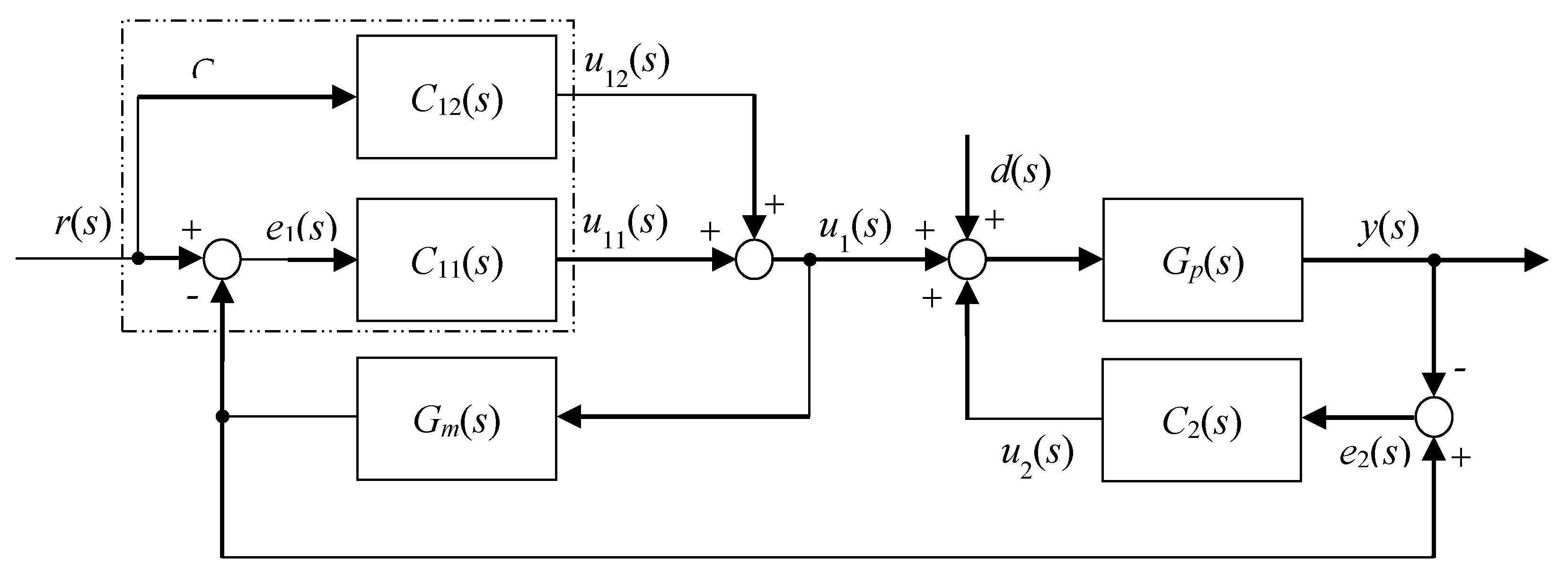
The modified 2-DOF framework proposed in this paper is shown in Figure 1.

Where e₁(s) is the error which is the difference between set-point input r(s) and model output y_m(s); e₂(s) is the error which is the difference between the model output y_m(s) and process output y(s); u_j(s) (j = 1,2) and d(s) denote the control inputs and load disturbance input, respectively. It is assumed that d(s) is immeasurable. G_p(s) and G_m(s) represent the plant and its model, respectively. C₁₁(s) and C₁₂(s) are controllers to implement the set-point weighted PID controller and C₁(s) and C₂(s) are the controllers that respond well to the load disturbance.

A unique feature of the proposed control framework is that a feedforward controller C₁₂(s) is embedded by modifying the parallel control structure reported by Karunagaran et al. [20]. The embedded feedforward controller C₁₂(s) is to implement the set-point weighting which is to speed up the response while reducing overshoot in the set-point tracking response.

For the sake of simplicity when developing the equation afterwards, the symbol s representing the Laplace domain is omitted and expressed.

In Figure 1,

$$\begin{gathered} y_m=G_m{u}_1, \\ {u}_1=C_{11}(r-y_m)+C_{12}r=\frac{C_{11}+C_{12}}{1+C_{11}{G}_m}r \\ {u}_2=C_2(y_m-y) \end{gathered}$$

(9)

If the output of the process is obtained using the relationship of Equation (9), it is expressed as in Equation (10).

$$\begin{array}{ll}y& =G_p(u_1+u_2+d)\\ & =\frac{(C_{11}+C_{12})G_p(1+C_2{G}_m)}{(1+C_{11}{G}_m)(1+C_2{G}_p)}r+\frac{G_p}{1+C_2{G}_p}d\end{array}$$

(10)

Under nominal conditions, i.e., when G_p = G_m, y can be expressed as

$$y=\frac{(C_{11}+C_{12})G_m}{1+C_{11}{G}_m}r+\frac{G_m}{1+C_2{G}_m}d$$

(11)

It can be observed from Equation (11) that the controllers C₁₁ and C₁₂ take care of the set-point tracking response, whereas load disturbances are rejected by the controller C₂. In this way, the proposed 2-DOF control framework can separate the load disturbance rejection response from the set-point tracking response. Thus, the ability to independently manipulate the set-point tracking and load disturbance rejection responses is established under nominal conditions.

As shown in Equation (11), the set-point weighted PID controller C₁ can be implemented by combining the feedforward controller C₁₂ with reference input and the controller C₁₁ with error input.

If C₁₁ is a PID controller in parallel form as Equation (12) and C₁₂ is given as Equation (13), the set-point weighted PID controller C₁ is implemented as Equation (14) by summing the output u₁₁ of controller C₁₁ and the output u₁₂ of controller C₁₂. The PID controller C₂ for load disturbance rejection is expressed as Equation (15).

$$C_{11}:u_{11}=k_{p1}{e}_1+k_{i1}\frac{1}{s}{e}_1+k_{d1}s{e}_1$$

(12)

$$C_{12}:u_{12}=-k_{p1}(1-\epsilon )r$$

(13)

$$u_1=k_{p1}(\epsilon r-y)+k_{i1}\frac{1}{s}{e}_1+k_{d1}s{e}_1$$

(14)

$$C_2:u_2=k_{p2}{e}_2+k_{i2}\frac{1}{s}{e}_2+k_{d2}s{e}_2$$

(15)

where k_pj (j = 1,2), k_ij (j = 1,2), and k_dj (j = 1,2) denote proportional, integral and derivative gains in the parallel PID controllers, respectively. ɛ denotes the set-point weighting parameter and ranges from 0 to 1. As such, the set-point weighted PID controller C₁ improves the set-point tracking performance, while the load disturbance is suppressed by the controller C₂.

From Equation (11), it is observed under process mismatch conditions that the controller C₁ composed of C₁₁ and C₁₂ has no influence on the disturbance rejection response at all. However, controller C₂ affects both set-point tracking and disturbance rejection responses. However, Karunagaran et al. [20] have reported that the control action of controller C₂ mainly influences the disturbance rejection response with minimal change in set-point tracking response.

3.2. GA Based Optimal Tuning

A brief summary of genetic algorithms is as follows. Evolutionary computation is a broad concept and includes genetic algorithms, evolution strategies and genetic programming. All of these techniques mimic evolution using operators such as reproduction, crossover, and mutation, etc. GA combines some of the features found in evolution with computer algorithms to solve complex optimization problems. GA does not require a prior knowledge of a searching space other than an objective function because it is free from constraints on the searching space such as continuity, differentiability and unimodality, etc. There is an advantage of using a solution population to converge toward the global solution even in a very large and complex space. GA is a statistical search algorithm based on biological evolution to create a population of individuals, evaluate the fitness of the individuals and create new individuals using genetic operators. The search process of the GA is divided into five stages: initialization of population, fitness evaluation, reproduction, crossover, and mutation. In this way, the newly formed population repeats the fitness evaluation, reproduction, crossover, and mutation operations until the optimal solution is found.

The two controllers mentioned above must be well-tuned to provide excellent performance for set-point tracking and load disturbance rejection, respectively. Since the proposed 2-DOF control framework can decouple the load disturbance rejection response from the set-point tracking response under nominal conditions, it can be tuned separately when tuning the parameters of each PID controller.

Figure 2 shows a block diagram for GA based optimal tuning of the set-point weighted PID controller C₁ and the disturbance rejection controller C₂.

When tuning the controller C₂, the reference r is considered r = 0 because it is usually fixed constant, and it is assumed that disturbance d changes stepwise. When tuning the controller C₁, it is assumed that the disturbance input d = 0 and the reference input r changes stepwise.

The performance of each controller depends on how the parameters are properly tuned in the controller. This is a multivariable optimization problem which is solved by GA in this paper.

While a population is evolving, the GA needs the fitness to evaluate the superiority of the individual population and the fitness is calculated from a performance index. ISE, IAE and ITAE are frequently used as performance indices that can quantify the performance of the system. Since ISE is easy to interpret, it is often used in the design of the optimal controller. This is insensitive to parameter changes near a minimum because it gives a large penalty for large errors and a small penalty for small errors due to the square of errors. On the other hand, IAE gives equal penalties for positive or negative errors by taking an absolute size of the error, indicating a slightly better sensitivity than ISE near the minimum. ITAE is more discriminative than ISE or IAE for the transient phenomenon of a long time.

In this paper, IAE is selected as performance index to evaluate the performance of each PID controller.

$$J({\varphi }_j)={\displaystyle {\int }_0^{t_f}\left|e_j\right|dt,(j=1,2)}$$

(16)

where ϕ_j(j = 1,2) is a vector composed of the tuning parameters and weighting factor of the PID controller, e_j(j = 1,2) are errors and t_f is a value sufficiently large enough time to ignore integral afterwards.

J(ϕ₁) and J(ϕ₂) are the performance indices for controllers C₁ and C₂, respectively. Where e₁ = r − y_m and e₂ = y_m − y are errors, ϕ₁ = [k_p, k_i, k_d, ɛ]^T∈R⁴ and ϕ₂ = [k_p, k_i, k_d]^T∈R³ are vectors composed of PID controller parameters and r is the set-point input, y the process output and y_m the model output.

ϕ_j(j = 1,2) are tuned by GA in terms of minimizing the IAE performance index in Equation (16).

For the control parameters of GA, P_size = 40 is considered for the population size, η_r = 1.7 for the reproduction coefficient, P_c = 0.9 for the crossover probability, P_m = 0.05 for the mutation rate and b = 5 for the dynamic mutation. Constraints used in the optimization problem are 0 ≤ k_p ≤ k_pm, 0 ≤ k_i ≤ k_im, 0 ≤ k_d ≤ k_dm and 0 ≤ ε ≤ 1.0, where k_pm, k_im and k_dm denote upper bound values of PID controller gains.

In general, since the accuracy and convergence speed of the solution obtained by GA varies depending on the selection of the initial population, each simulation is performed five times using the initial population created as an independent seed, and the results obtained here are averaged.

3.3. GA Based Model Reduction

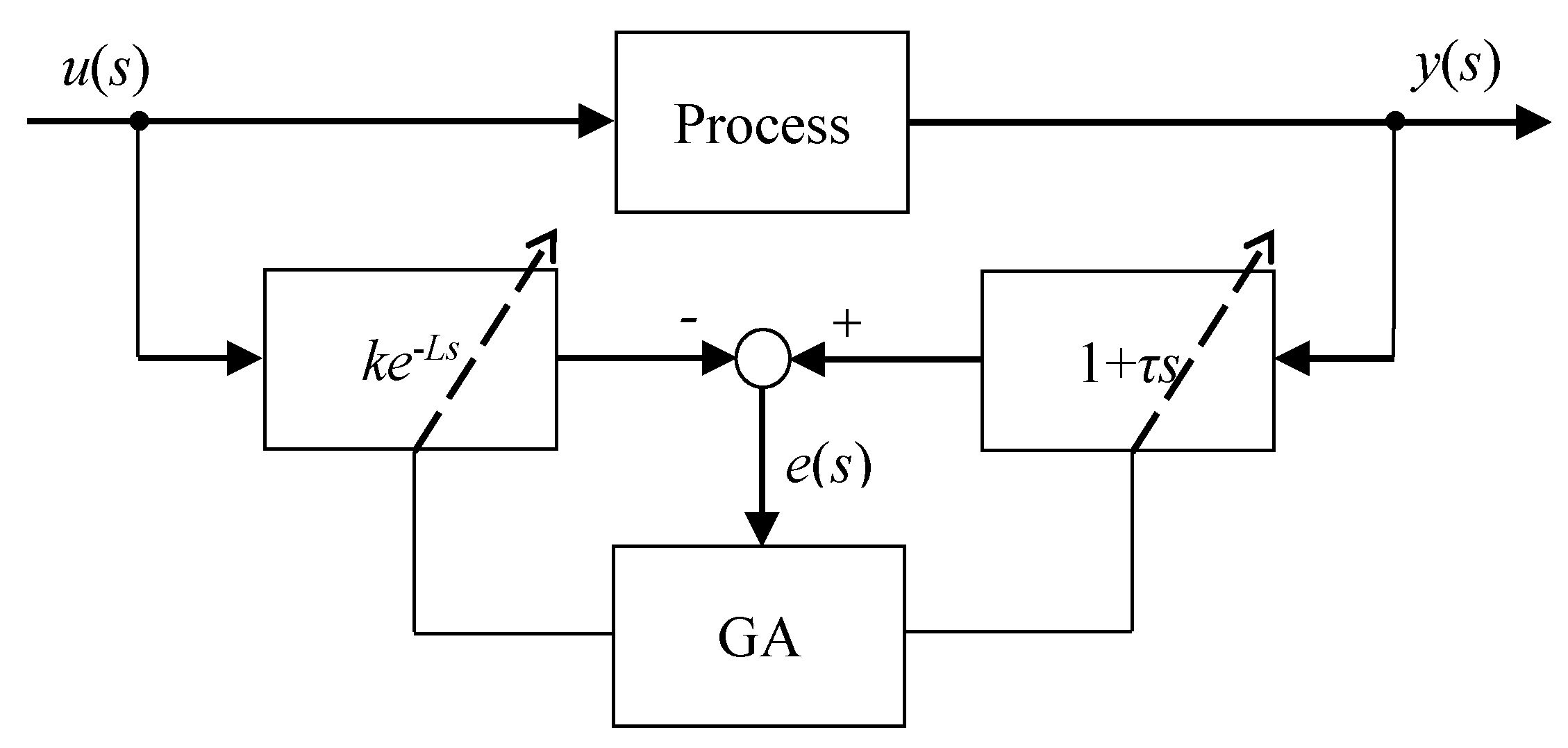
Figure 3 shows a block diagram for GA based approximate model reduction [31].

Where e is the error, u and y denote input and process output, respectively.

When there is a discrepancy between a process and a model, the following error occurs from the FOPTD model (Equation (1)).

$$e=(1+\tau s)y-k{e}^{-Ls}u$$

(17)

When the same input is applied to a model that is linked in parallel with the process, the genetic algorithm uses a pair of input and output data to continuously adjust three parameters of the model so that the dynamic characteristics of the model are closer to that of the process, in terms of minimizing the IAE performance index in Equation (18).

$$J({\varphi }_M)={\displaystyle {\int }_{(m-w+1)h}^{mh}\left|e\right|dt}$$

(18)

where ${\varphi }_M={[k,\tau ,L]}^T\in R^3$ and h are parameter vectors to be adjusted and sampling time, respectively. $W$ is the size of a data window, which is an appropriately compromised parameter between accuracy and time of operation.

Because the performance index is calculated in a finite amount of time, $W$ input and output data pairs {u(m), y(m)} must be stored in the buffer to drive the model. One additional input and output pair is also required to initialize the model. Figure 4 shows the data buffer. Whenever a new pair of data is obtained, the contents of the buffer are moved and updated.

4. Simulation and Review

To verify the effectiveness of the proposed 2-DOF control framework and PID controllers in it, a set of simulation works on four virtual processes are performed. The conventional PID controllers by TK-IAE and SG-IMC are designed and simulated after approximating the given processes into a FOPTD model using GA, and JIN-NPID applies the tuning rules to his proposed nonlinear PID controller for simulation.

The servo and regulatory response performances for the proposed method are compared with those of the PID controllers by JIN-NPID, TK-IAE, and SG-IMC for four processes.

For quantitative comparison in each simulation work, performance measures such as rise time t_r = t₉₅ − t₅, 2% settling time t_s, percentage overshoot M_p and integral of absolute error IAE for set-point tracking performance and peak time t_peak, recovery time t_rcy, maximum peak error M_peak, and integral of absolute error IAE for load disturbance rejection performance are calculated. The overall performance evaluation is performed based on IAE considering t_r, t_s, t_peak, M_p, M_peak and t_rcy. The smaller the IAE value, the better the overall performance.

4.1. Process 1

First, the second-order process with time delay shown in Equation (19) is considered:

$$G_p(s)=\frac{e^{-2s}}{(1+10s)(1+s)}$$

(19)

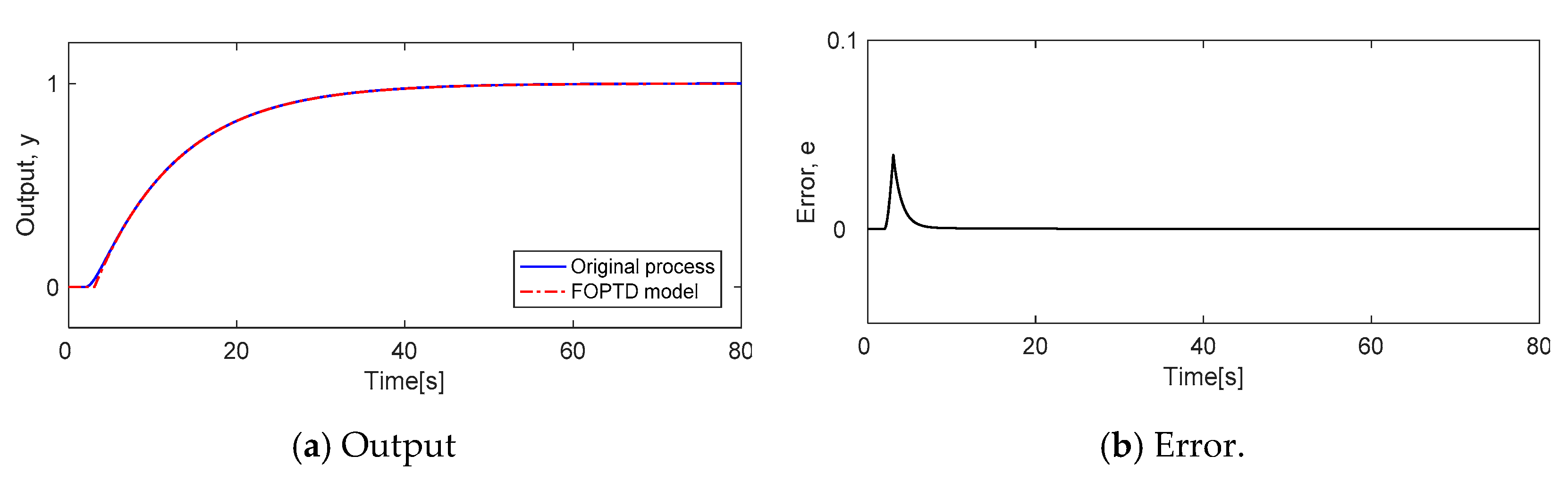
The parameters of the FOPTD model from process 1 by the GA based model reduction technique [31] are given as k = 1, τ = 10.002, and L = 3.06. It can be seen that in this case L/τ ≒ 0.31 (<1).

Figure 3 shows the outputs and their errors when a unit step input is applied to the original process and the approximate FOPTD model. As shown in Figure 5, the approximated model is almost consistent with the original process.

The parameters of controllers C₁ and C₂ were tuned using the control parameters for GA described in the previous section and the given constraints for the search space.

Constraints used for the search space in the optimization problem are 0 ≤ k_p ≤ 3.2, 0 ≤ k_i ≤ 1.0, 0 ≤ k_d ≤ 3.8 and 0 ≤ ε ≤ 1.0.

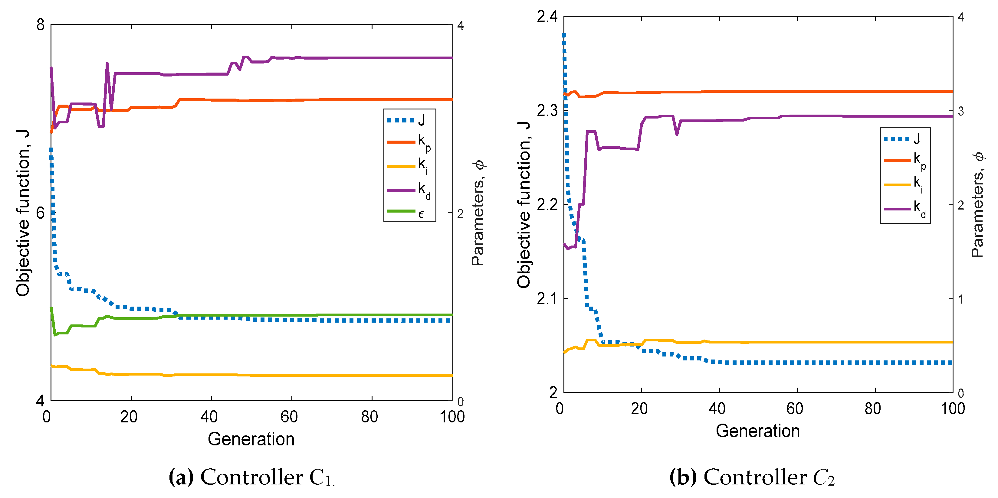
Figure 6 shows the tuning process for PID controllers C₁ and C₂, respectively. As shown in Figure 6, the solutions are found at approximately 55 generations and 60 generations, respectively.

The tuning results of controllers C₁ and C₂ by GA and those of conventional PID controllers by other methods using Equations (5)–(7) are listed in

Table 1. PID controller tuning for process 1.

Tuning Method		Parameters
		kp	ki	kd	Remarks
Proposed	C1	3.1996	0.2697	3.6854	ε = 0.9121
	C2	3.1999	0.5361	2.9367
JIN-NPID		3.1238	0.3157	3.6170
TK-IAE		1.9765	0.1930	0.2196
SG-IMC		1.6343	0.1634	0

.

Simulation work was carried out to demonstrate the set-point tracking and load disturbance rejection performances of the proposed method.

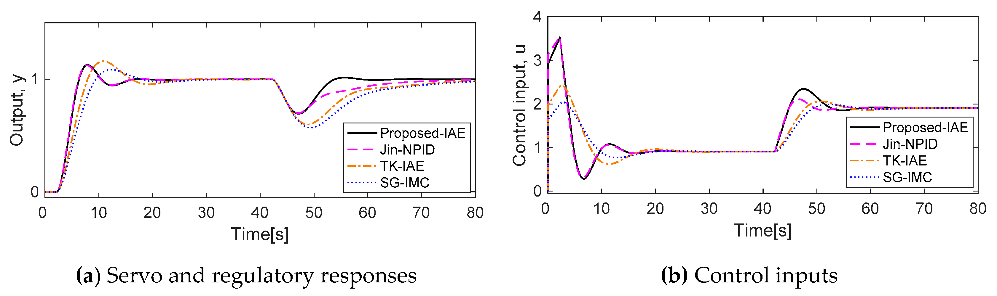
A unit step input in the set-point at t = 0 and a negative unit step input in the load disturbance at t = 40 were introduced to the nominal process 1, and the servo and regulatory responses are shown in Figure 7. The performance measures for quantitative comparison are calculated and listed in

Table 2. Quantitative comparison of performances for nominal process 1.

Tuning Method	Tracking Performance				Disturbance Performance
	tr	Mp	ts	IAE	tpeak	Mpeak	trcy	IAE
Proposed	3.8050	2.0161	9.5387	4.8418	7.4600	0.2627	24.067	2.0322
JIN-NPID	3.7425	2.0390	9.6688	4.8471	7.5200	0.2585	39.512	3.1916
TK-IAE	5.1131	8.5079	23.586	6.2098	9.3800	0.3519	36.560	4.4394
SG-IMC	6.4705	3.8457	19.466	6.6308	10.040	0.3782	36.942	5.1976

.

As shown in Figure 7 and Table 2, the proposed scheme and JIN-NPID give fast set-point responses which are very similar, whereas the proposed method shows much shorter recovery times t_rcy than that of JIN-NPID. Therefore, the proposed method and JIN-NPID show similar performances in the set-point tracking response, but the proposed method is much better in the disturbance rejection response.

In particular, SG-IMC and TK-IAE show a very long settling time t_s in set-point tracking response and a very long recovery time t_rcy in disturbance rejection response. Moreover, SG-IMC and TK-IAE also have very large maximum peak errors M_peak. The IAE values are also smaller in the order of the proposed method, JIN-NPID, TK-IAE and SG-IMC. Therefore, the proposed method has the best performance. On the contrary, SG-IMC has the worst.

The parameters in the process may change during operations. The robustness is investigated by simultaneously inserting a perturbation uncertainty of 10% into all four parameters in the worst direction and assuming the actual process as G_p(s) = 1.1e^−2.2s/[(1 + 9s)(1 + 0.9s)]. The process outputs and corresponding control inputs by the four methods for the process mismatch are given in Figure 8. The performance measures for quantitative comparison are calculated and listed in

Table 3. Quantitative comparison of performances for process 1 under 10% mismatch.

Tuning Method	Tracking Performance				Disturbance Performance
	tr	Mp	ts	IAE	tpeak	Mpeak	trcy	IAE
Proposed	2.8244	12.026	14.848	5.0021	7.1400	0.3069	22.780	1.9545
JIN-NPID	2.8584	12.268	14.826	5.0258	7.1000	0.3003	38.879	3.1943
TK-IAE	3.9795	16.036	23.216	6.2772	8.8200	0.4014	44.927	5.0145
SG-IMC	4.9464	8.4793	24.318	6.3916	9.3800	0.4288	45.956	5.9134

.

As shown in Figure 8, all four methods give slightly increased overshoots for parameter changes than those in the case of the nominal process. The proposed method and JIN-NPID give fast set-point responses with small overshoots, whereas JIN-NPID has a very long t_rcy. In particular, TK-IAE and SG-IMC show a very long t_rcy and a very large M_peak. These can also be confirmed by the quantitative results shown in Table 3, where the IAE values are smaller in the order of the proposed method, JIN-NPID, TK-IAE and SG-IMC. Therefore, the proposed method has the best response and SG-IMC has the worst.

4.2. Process 2

Second, the third-order process with time delay is considered:

$$G_p(s)=\frac{e^{-s}}{(1+0.5s)(1+s)(1+2s)}$$

(20)

where k = 1.001, τ = 2.306 and L = 2.32 were obtained as the FOPTD model parameters. It can be seen that L/τ ≒ 1.006 (≈1) in this case.

Table 4. PID controller tuning for process 2.

Tuning Method		Parameters
		kp	ki	kd	Remarks
Proposed	C1	1.0999	0.2854	0.9369	ε = 0.9999
	C2	1.0999	0.3985	0.7871
JIN-NPID		1.0775	0.4269	0.8311
TK-IAE		0.8283	0.2582	0.0212
SG-IMC		0.4965	0.2153	0

shows the results tuned by GA under the constraints of the search spaces 0 ≤ k_p ≤ 1.1, 0 ≤ k_i ≤ 0.5, 0 ≤ k_d ≤ 1.0 and 0 ≤ ε ≤1.0 and those of conventional PID controllers by other methods.

The simulation results for a unit step change in the set-point at t = 0 and a negative unit step disturbance at t = 40 in the nominal process are presented in Figure 9. The performance measures for quantitative comparison are calculated and tabulated in

Table 5. Quantitative comparison of performances for nominal process 2.

Tuning Method	Tracking Performance				Disturbance Performance
	tr	Mp	ts	IAE	tpeak	Mpeak	trcy	IAE
Proposed	3.0348	1.2567	5.9029	3.5366	5.0200	0.5308	15.574	2.6956
JIN-NPID	3.1463	4.5759	11.129	3.7792	5.0000	0.5282	16.895	2.7818
TK-IAE	3.3174	7.5885	16.107	4.2579	5.5800	0.6280	21.402	3.8673
SG-IMC	4.9027	4.0781	14.125	4.991	6.0400	0.6813	14.865	4.7366

.

As shown in Figure 9 and Table 5, the proposed method is far superior to others in both M_p and t_s in set-point tracking response and shows similar response to JIN-NPID in disturbance rejection response. In particular, SG-IMC has a long t_r in its set-point tracking response and TK-IAE shows also a large M_p in set-point tracking response and a long t_rcy in disturbance rejection response, respectively. The IAE values are also smaller in the order of the proposed method, JIN-NPID, TK-IAE and SG-IMC. Therefore, the proposed method gives the best performance. On the contrary, SG-IMC gives the worst.

The robustness was evaluated by simultaneously inserting 10% perturbations into each the nominal process parameters towards the worst case process mismatch and assuming the actual process to be G_p(s) = 1.1e^−1.1s/[(1 + 0.45s)(1 + 0.9s)(1 + 1.8s)]. The simulation results for the process mismatch are given in Figure 10. The performance measures for quantitative comparison are calculated and listed in

Table 6. Quantitative comparison of performances for process 2 under 10% mismatch.

Tuning Method	Tracking Performance				Disturbance Performance
	tr	Mp	ts	IAE	tpeak	Mpeak	trcy	IAE
Proposed	2.3757	4.2530	9.1765	3.3012	4.6999	0.5983	11.201	2.5666
JIN-NPID	2.4810	5.2032	8.0239	3.3713	4.6800	0.5953	10.796	2.6832
TK-IAE	2.7121	12.701	14.758	4.1886	5.2600	0.7083	19.572	3.8670
SG-IMC	4.0918	5.0366	12.068	4.5649	5.6600	0.7638	13.240	4.6942

.

As shown in Figure 10, the proposed method and JIN-NPID show almost the same level of excellent performance overall, but TK-IAE has a particularly large M_p and a long t_s in the set-point tracking response, and a very long t_rcy in the disturbance rejection response.

These can also be confirmed by the quantitative results shown in Table 6, where the IAE values are smaller in the order of the proposed method, JIN-NPID, TK-IAE and SG-IMC. Therefore, the proposed method has the best response and SG-IMC has the worst.

4.3. Process 3

Third, the third-order process with a double pole and time delay, shown in Equation (21), is considered:

$$G_p(s)=\frac{e^{-5s}}{{(1+s)}^2(1+2s)}$$

(21)

where k = 1.002, τ = 2.497 and L = 6.64 were obtained as the FOPTD model parameters. It can be seen that L/τ ≒ 2.66 (>1).

The tuning results by the proposed method under the constraints which are the search spaces 0 ≤ k_p ≤ 0.7, 0 ≤ k_i ≤0.5, 0 ≤ k_d ≤ 1.2 and 0 ≤ ε ≤1.0 and those of conventional PID controllers by other methods are listed in

Table 7. PID controller tuning for process 3.

Tuning Method		Parameters
		kp	ki	kd	Remarks
Proposed	C1	0.6002	0.1076	1.1789	ε = 0.9999
	C2	0.6677	0.1302	1.1590
JIN-NPID		0.6310	0.1641	1.0237
TK-IAE		0.3491	0.0721	0.0097
SG-IMC		0.1877	0.0752	0

.

The servo and regulatory responses for a unit step change introduced in both the set-point at t = 0 and load disturbance at t = 80 in the nominal process are given in Figure 11.

The performance measures for quantitative comparison are calculated and listed in

Table 8. Quantitative comparison of performances for nominal process 3.

Tuning Method	Tracking Performance				Disturbance Performance
	tr	Mp	ts	IAE	tpeak	Mpeak	trcy	IAE
Proposed	5.5822	3.9749	23.125	9.7354	12.300	0.8729	25.384	7.9086
JIN-NPID	5.6121	4.2504	19.478	9.6273	12.360	0.8759	35.148	8.2827
TK-IAE	14.571	0	41.948	13.846	13.500	0.9216	51.566	13.764
SG-IMC	12.778	3.5428	39.111	14.243	13.940	0.9337	48.752	14.151

.

As shown in Figure 11, the proposed method and JIN-NPID show almost the same level of excellent performance overall with small overshoots, whereas TK-IAE and SG-IMC show particularly large t_r and long t_s in their set-point tracking responses, and very long t_rcy in disturbance rejection responses. As shown in Table 8, the IAE values are smaller in the order of JIN-NPID, the proposed method, TK-IAE and SG-IMC for the servo response, whereas the order is the proposed method, JIN-NPID, TK-IAE and SG-IMC for the regulatory response. Therefore, the proposed method and JIN-NPID have the best responses and SG-IMC has the worst.

The robustness of the proposed scheme was assessed by simultaneously inserting 10% perturbations into all four parameters of the nominal process towards the worst case process mismatch and assuming the actual process to be G_p(s) = 1.1e^−5.5s/[(1 + 0.9s)²(1 + 1.8s)]. The simulation results for the process mismatch are given in Figure 12. The performance measures for quantitative comparison are calculated and listed in

Table 9. Quantitative comparison of performances for process 3 under 10% mismatch.

Tuning Method	Tracking Performance				Disturbance Performance
	tr	Mp	ts	IAE	tpeak	Mpeak	trcy	IAE
Proposed	4.5980	16.214	33.043	10.411	12.680	1.0042	41.390	9.3829
JIN-NPID	4.5923	15.627	30.066	10.584	12.740	1.0062	33.706	9.0071
TK-IAE	9.3736	0	38.571	12.589	13.720	1.0399	48.115	13.825
SG-IMC	10.598	7.8104	38.650	14.040	14.080	1.0486	48.089	15.276

.

As shown in Figure 12 and Table 9, the proposed method and JIN-NPID show almost the same level of excellent performance overall with small overshoots, but TK-IAE and SG-IMC show particularly large t_r and long t_s in the set-point tracking response, and very long t_rcy in the disturbance rejection response.

As shown in Table 9, the IAE values are smaller in the order of the proposed method, JIN-NPID, TK-IAE and SG-IMC for the servo response, but JIN-NPID, the proposed method, TK-IAE and SG-IMC for the regulatory response. Therefore, the proposed method provides the highest robustness for set-point tracking response, whereas JIN-NPID has the best regulatory response. On the contrary, SG-IMC gives the worst.

4.4. Process 4

Finally, the fourth-order process with a quadruple pole and time delay shown in Equation (22) is considered:

$$G_p(s)=\frac{e^{-8s}}{{(1+s)}^4}$$

(22)

where k = 1.001, τ = 2.093, and L = 10.08 were obtained as the FOPTD model parameters by the GA based model reduction technique. It can be seen that L/τ ≒ 4.816 (>3).

The tuning results by the proposed method under the constraints which are the search spaces 0 ≤ k_p ≤ 0.7, 0 ≤ k_i ≤ 0.5, 0 ≤ k_d ≤ 1.2, and 0 ≤ ε ≤ 1.0 and those of conventional PID controllers by other methods are listed in

Table 10. PID controller tuning for process 4.

Tuning Method		Parameters
		kp	ki	kd	Remarks
Proposed	C1	0.4650	0.0728	0.9886	ε = 0.9200
	C2	0.4999	0.0819	0.9999
JIN-NPID		0.4558	0.1027	0.9299
TK-IAE		0.1992	0.0366	0.0046
SG-IMC		0.1037	0.0496	0

.

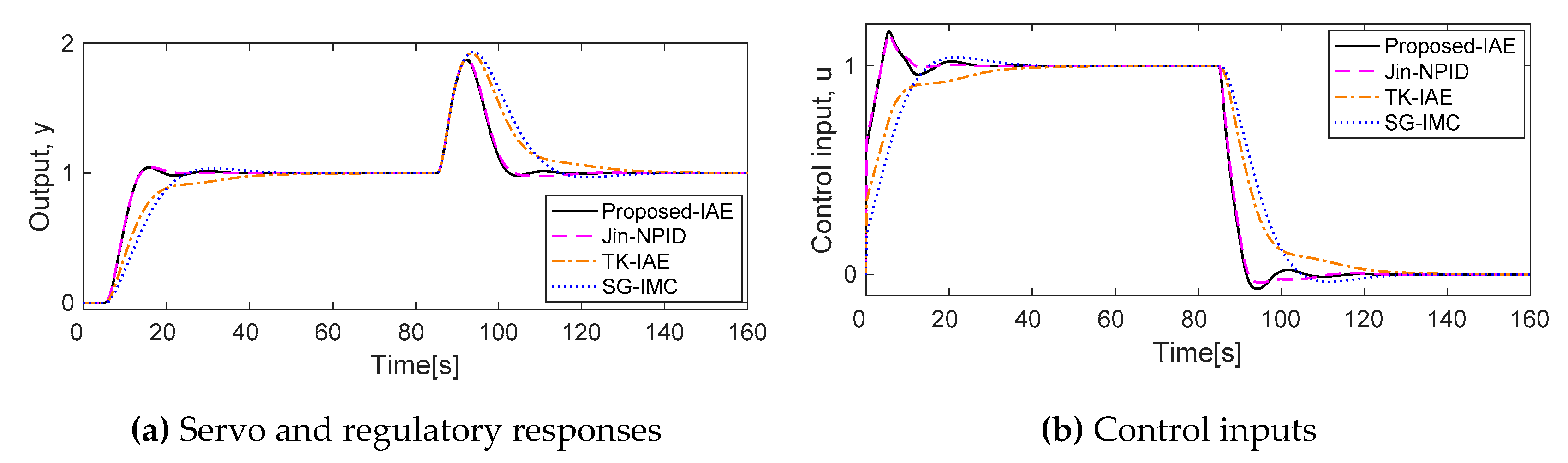
The servo and regulatory responses for a unit step change introduced in both the set-point at t = 0 and load disturbance at t = 160 in the nominal process are given Figure 13.

The performance measures for quantitative comparison are calculated and listed in

Table 11. Quantitative comparison of performances for nominal process 4.

Tuning Method	Tracking Performance				Disturbance Performance
	tr	Mp	ts	IAE	tpeak	Mpeak	trcy	IAE
Proposed	8.2505	1.2803	32.748	14.402	17.900	0.9860	37.696	12.558
JIN-NPID	7.9324	1.5500	37.099	14.598	17.920	0.9861	45.979	13.330
TK-IAE	41.741	0	86.254	27.309	18.880	0.9925	97.534	21.174
SG-IMC	19.640	3.1322	59.041	21.697	19.140	0.9937	71.123	21.681

.

As shown in Figure 13, the proposed method and JIN-NPID show almost the same level of excellent performance overall with small overshoots, but TK-IAE and SG-IMC show a particularly large t_r and a long t_s in the set-point tracking response, and a very long t_rcy in the disturbance rejection response. As shown in Table 11, the IAE values are smaller in the order of the proposed method, JIN-NPID, SG-IMC and TK-IAE for the servo response, and smaller in the order of the proposed method, JIN-NPID, TK-IAE and SG-IMC for the regulatory response. Therefore, the proposed method has the best response and TK-IAE has the worst.

The robustness was evaluated by inserting a perturbation uncertainty of 10% in the gain, time delay and time constant in the worst direction such that G_p(s) = 1.1e^−8.8s/(1 + 0.9s)⁴.

The perturbed responses are shown in Figure 14. The simulation results for the process mismatch are given in

Table 12. Quantitative comparison of performances for process 4 under 10% mismatch.

Tuning Method	Tracking Performance				Disturbance Performance
	tr	Mp	ts	IAE	tpeak	Mpeak	trcy	IAE
Proposed	6.9633	13.618	30.714	15.301	18.900	1.0946	51.983	15.064
JIN-NPID	6.5157	12.178	55.554	15.428	18.920	1.0946	63.821	15.065
TK-IAE	34.784	0	74.754	24.832	19.680	1.0969	87.047	27.283
SG-IMC	16.326	8.0751	60.474	21.743	19.880	1.0974	73.023	23.860

.

As shown in Figure 14, the proposed method and JIN-NPID show almost the same level of excellent performance overall with small overshoots, but TK-IAE and SG-IMC show particularly large t_r and a long t_s in the set-point tracking response, and very long t_rcy in the disturbance rejection response.

As shown in Table 12, the IAE values are smaller in the order of the proposed method, JIN-NPID, SG-IMC and TK-IAE for both servo and regulatory responses. Therefore, the proposed method gives the best response. On the contrary, TK-IAE gives the worst.

5. Conclusions

In this paper, a modified 2-DOF control framework was proposed to overcome the contradiction between servo and disturbance rejection responses, with a discussion on how to optimally tune each parameter of the two controllers within the control framework.

There are three remarkable features: one is that the modified 2-DOF control framework decouples the regulatory response from the servo response under nominal conditions; another is that the standard PID controller and feedforward controller, which has proportional action function, are combined to create a new set-point weighted PID controller for improving the set-point tracking performance; the other is that the set-point weighting factor within the set-point weighted PID controller is also tuned simultaneously when tuning the controller. Each controller was optimally tuned by GA in terms of minimizing the IAE performance index with the constraints of a given search space under nominal conditions.

To validate the proposed scheme, the set-point tracking and disturbance rejection response performances for step input, and the robustness for parameter uncertainties of the processes were measured. The performance measures such as t_r, t_s, M_p and IAE for set-point tracking, and such as t_peak, M_peak, t_rcy, and IAE for disturbance rejection were used.

The proposed method was applied to control the four virtual processes and its performance and robustness were compared with those of JIN-NPID, TK-IAE and SG-IAE. The simulation results showed that the performance and robustness by the proposed method were much better than those of TK-IAE and SG-IAE methods but showed almost the same level of excellent performance with JIN-NPID.

Future studies will focus on adding the antiwind up function of integral action and expanding into processes with conjugate complex poles, positive or negative zero.