A Novel Hybrid Model Based on an Improved Seagull Optimization Algorithm for Short-Term Wind Speed Forecasting

Abstract

Wind energy is a clean energy source and is receiving widespread attention. Improving the operating efficiency and economic benefits of wind power generation systems depends on more accurate short-term wind speed predictions. In this study, a new hybrid model for short-term wind speed forecasting is proposed. The model combines variational modal decomposition (VMD), the proposed improved seagull optimization algorithm (ISOA) and the kernel extreme learning machine (KELM) network. The model adopts a hybrid modeling strategy: firstly, VMD decomposition is used to decompose the wind speed time series into several wind speed subseries. Secondly, KELM optimized by ISOA is used to predict each decomposed subseries. The ISOA technique is employed to accurately find the best parameters in each KELM network such that the predictability of a single KELM model can be enhanced. Finally, the prediction results of the wind speed sublayer are summarized to obtain the original wind speed. This hybrid model effectively characterizes the nonlinear and nonstationary characteristics of wind speed and greatly improves the forecasting performance. The experiment results demonstrate that: (1) the proposed VMD-ISOA-KELM model obtains the best performance for the application of three different prediction horizons compared with the other classic individual models, and (2) the proposed hybrid model combining the VMD technique and ISOA optimization algorithm performs better than models using other data preprocessing techniques.

1. Introduction

To achieve global clean energy development, reduce greenhouse gas emissions and prevent the crisis of the depletion of nonrenewable fossil energy reserves, the large-scale use of clean energy has become a global energy development trend [1,2]. Among the various widely used new energies, wind energy is used worldwide due to its wide energy distribution, pollution-free nature and sustainability, and it is of great significance to tap into the potential of wind energy to adjust the traditional energy structure. According to a report released by the Global Wind Energy Association (GWEC) in 2019, the global installed capacity of wind power in 2019 was 60.4 GW, reaching a total of 651 GW. As of the end of 2019, China’s cumulative installed wind power capacity reached 210 MW [3]. The chaotic, random and intermittent characteristics of wind speed pose considerable challenges to power systems. The violent fluctuation of wind power in a short period of time causes a short-term imbalance of the power system, which may cause the power system to collapse. Therefore, accurate wind speed forecasting is critical to accurately predicting the output power of wind power and stabilizing the operating state of the power system.

At present, wind speed prediction methods mainly include the following four methods: (i) the physical model method, (ii) the time series method, (iii) the spatial correlation method and (iv) the artificial intelligence method [4,5,6]. The physical model method mainly uses the physical parameters when the wind speed generates the background to construct complex mathematical equations, and uses numerical weather prediction (NWP) for simulation. Classic numerical simulation approaches include the high-resolution limited area model (HIRLAM) [7], the fifth-generation mesoscale model (MM5) [8] and the weather research and forecast model (WRF) [9]. However, physical methods have disadvantages such as a difficulty in obtaining physical data, the consumption of many computing resources and being unsuitable for short-term wind speed prediction [10]. The time series method uses the potential before and after information and correlation in the historical wind speed data to build a model. Common wind speed statistical models include autoregressive (AR) [11], autoregressive moving average (ARMA) [12], autoregressive integrated moving average (ARIMA) [13] and autoregressive fraction moving average (ARFIMA) [14] models. Although time series approaches are simpler and more economical when compared with physical model methods, they are also limited by the nonlinearity and nonstationarity of the wind speed time series. As a unique method, the spatial correlation model starts from the relevant wind speed data around the wind speed center and selects appropriate sites to build a spatial model. Samalot et al. [15] successfully combined Kalman filtering and Kriging to reduce the bias of the weather research and forecasting (WRF) model. However, this method has strict measurement requirements and is difficult to implement.

In addition, with the rise of artificial intelligence, artificial intelligence methods have shown strong advantages in the extraction of the nonlinear characteristics of wind speed fluctuations, and have gradually become a research hotspot in the field of prediction. Many methods including artificial neural networks (ANNs) [16,17], support vector machines (SVMs) [18,19] and fuzzy logic (FL) methods [20,21] have been applied to wind speed prediction. Monfared et al. [22] combined fuzzy logic with an artificial neural network, which not only effectively reduced the rule base but also improved the accuracy of predicting wind speed. Li et al. [23] studied the application of adaptive linear elements (ALEs), back propagation (BP) and radial basis functions (RBFs) to these three neural networks in 1-h wind speed prediction and proposed that the best prediction model is related not only to the type of neural network but also to the data source. Guo et al. [24] proposed a backpropagation neural network wind speed prediction method to eliminate seasonal effects to predict daily average wind speed. This method can effectively eliminate seasonal effects from actual wind speed data. Zhang et al. [25] proposed a two-step method to determine the connection weight of the RBF network to predict the future wind speed interval. Compared with the traditional multilayer perceptron (MLP) method, this method can effectively increase the prediction interval. Compared with the traditional neural network, the extreme learning machine (ELM) has faster convergence speed and less human intervention, which leads to its strong generalization ability for heterogeneous datasets [26].

The neural network improves the prediction accuracy of wind speed series to a certain extent. However, the instability of the wind speed sequence and the corresponding noise also create considerable interference in the neural network model training process. In the end, the model training effect is not good, and the wind speed prediction error is large. Therefore, to solve the random interference of the wind speed sequence, various preprocessing technologies have been developed. Liu et al. [27] used wavelet transform (WT) preprocessing technology to decompose the original sequence into multiple wind velocity subsequences, and then made predictions through the echo state network. Niu et al. [28] used empirical mode decomposition (EMD) to decompose the original signal and then predicted each subsequence through the general regression neural network (GRNN) optimized by the fruit fly algorithm (FOA), which improved the accuracy of wind prediction. EMD cannot effectively decompose the original wind speed series due to its disadvantages such as end effects and modal aliasing. After that, Ren et al. [29] studied the prediction model based on EMD, its improved version and two intelligent algorithms, and finally suggested complete ensemble empirical mode decomposition with adaptive noise (CEEMDAN)and support vector regression (SVR) as the best wind speed prediction method. Zhou et al. [30] proposed a hybrid framework for multilevel wind speed prediction based on variational model decomposition (VMD) and convolutional neural networks. Furthermore, chaos theory has increasingly attracted attention. Multifractal patterns of wind speed can be obtained through chaotic characteristics analysis. Jiang et al. [31] employed a hybrid linear-nonlinear modeling method based on chaos theory to capture the linear and nonlinear factors hidden in wind speed time series, which contained VMD technology to remove the noise in original data. The experimental results showed that the hybrid model was more accurate compared with other models.

Based on the analysis above, artificial intelligence methods have been the most extensive and successful approaches to short-term wind speed prediction, but the prediction ability of a single artificial intelligence method is limited. Hybrid approaches have shown better performance than single models. Therefore, it has gradually become a popular trend to apply data preprocessing techniques before sending wind speed data into forecasting models.

In this study, a novel hybrid strategy is proposed that includes three portions: data preprocessing, optimization and forecasting. Specifically, based on the decomposition and integration strategy, VMD decomposition is used to decompose the original wind speed series into several variational modes to filter out the noise in the original wind speed time series. Then, the KELM prediction network is applied to the problem of wind speed forecasting. At the same time, the improved seagull optimization algorithm is used to optimize the kernel parameters of the KELM network, thereby forming a hybrid model.

The main contributions and innovations of this research are as follows: (1) data preprocessing technology is included to reduce the volatility and randomness of wind speed series and improve the accuracy of prediction. VMD decomposes the original wind speed series into a set of relatively stable modes. (2) In the prediction phase, the kernel function is added to ELM to map the one-dimensional wind speed sequence to the high-dimensional space for prediction, which reduces the difficulty of prediction. (3) An improved seagull optimization algorithm (ISOA) is proposed to determine the two best parameters in KELM simultaneously. In the prediction phase, ISOA continuously searches for the two parameters of the kernel function in KELM. At the same time, each search can retain the optimal approximate solution, so that the KELM network can be optimized, and the prediction accuracy and stability of the prediction are improved. (4) A systematic assessment system is established to evaluate the forecasting ability of our developed hybrid model. Four multistep prediction experiments and three performance indicators are included in this study to compare and analyze the forecasting capacity of the proposed hybrid model in each case.

2. Methods

The technologies used in the hybrid strategy are introduced in this section, including the data preprocessing technology (VMD), the KELM network and the improved seagull optimization algorithm. In the last part, the workflow of the hybrid strategy is presented.

2.1. Variational Mode Decomposition (VMD)

VMD is a novel signal decomposition method that was proposed by Dragomiretskiy and Zosso in 2014 [32], which decomposes a one-dimensional signal into a limited number of modes with a center frequency bandwidth through an iterative search. VMD has good adaptive ability and can overcome modal aliasing. It can decompose nonstationary wind speed time series into subseries called intrinsic mode functions (IMFs). Each subseries contains rich information. The mathematical model of VMD can be expressed as follows:

$$\{\begin{array}{c}\underset{\left\{u_k\},\{{\omega }_k\right\}}{\min }\left\{{{\displaystyle \sum _k\Vert {\partial }_t\left[\left(\delta (t)+\frac{j}{\pi t}\right)u_k(t)\right]e^{-j{\omega }_{k}t}\Vert }}_2^2\right\}\\ s.t. {\displaystyle \sum _k{u}_k=f}\end{array},$$

(1)

where $f$ is the signal to be decomposed, $\delta (t)$ is the impulse function and $u_k$ and ${\omega }_k$ are the $k$-th mode component and the corresponding center frequency, respectively.

To solve the optimization problem of Formula (1), we introduce the terms of the Lagrange multiplier operator $\lambda$ and quadratic penalty factor $\alpha$:

$$L(u_k,{\omega }_k,\lambda )=\alpha {{\displaystyle \sum _k\Vert {\partial }_t\left[\left(\delta (t)+\frac{j}{\pi t}\right)u_k(t)\right]e^{-j{\omega }_{k}t}\Vert }}_2^2+{\Vert f-{\displaystyle \sum _{k=1}^K{u}_k}\Vert }_2^2+\langle \lambda ,f-{\displaystyle \sum _{k=1}^K{u}_k}\rangle ,$$

(2)

The following shows the whole process of VMD decomposition:

Step 1: Set the initial values of $\{{\widehat{u}}_k^1\}$, $\left\{{\omega }_k^1\right\}$, $\{{\widehat{\lambda }}^1\}$ and n, where ^ uses the Parseval/Plancherel Fourier equidistant transform for conversion to the frequency domain.

Step 2: Use Equations (3)–(5) to update $\{{\widehat{u}}_k^1\}$, $\left\{{\omega }_k^1\right\}$ and $\{{\widehat{\lambda }}^1\}$, respectively;

$${\widehat{u}}_k^{n+1}(\omega )=\frac{f\left(\omega \right)-{\displaystyle \sum _{i\ne k}{\widehat{u}}_i(\omega )+\frac{\lambda (\omega )}{2}}}{1+2\alpha {(\omega -{\omega }_k)}^2},$$

(3)

$${\omega }_k^{n+1}(\omega )=\frac{{\displaystyle {\int }_0^{\infty }\omega {\left|{\widehat{u}}_k(\omega )\right|}^{2}d\omega }}{{\displaystyle {\int }_0^{\infty }{\left|{\widehat{u}}_k(\omega )\right|}^{2}d\omega }},$$

(4)

$${\widehat{\lambda }}^{n+1}(\omega )={\lambda }^n(\omega )+\tau \left(f(\omega )-{\displaystyle \sum _k{u}_k^{n+1}(\omega )}\right),$$

(5)

Step 3: Go to step 2. until the iterative stop condition of Equation (6) is satisfied and output the result.

$${\displaystyle \sum _k\frac{{\Vert {\widehat{u}}_k^{n+1}-{\widehat{u}}_k^n\Vert }^2}{{\Vert {\widehat{u}}_k^n\Vert }^2}}<e.$$

(6)

2.2. Kernel Extreme Learning Machine

KELM is a single hidden layer feedforward neural network (SLFN). Traditional feedforward neural network training speed is slow and easily falls into local minimums, and the selection of the learning rate is sensitive. ELM randomly generates the connection weight between the input layer and the hidden layer and the threshold of the hidden layer source to obtain a unique optimal solution. For N arbitrarily distinct samples $(x_i,o_i)$, where $x_i={[x_{i1},x_{i2},\cdots ,x_{im}]}^T\in R^n$ and $o_i={[o_{i1},o_{i2},\cdots ,o_{im}]}^T\in R^m$, the output of an ELM with $L$ hidden neurons can be expressed as

$$\mathsf{\Theta }(x_i)={\displaystyle \sum _{i=1}^L{\beta }_{i}g(a_i\cdot x_j+b_i)=o_j, j=1,2,\dots ,N},$$

(7)

where $g(\cdot )$ represents the activation function of the hidden layer, $a_i={[a_{i1},a_{i2},\cdots ,a_{im}]}^T$ is the input weight vector, ${\beta }_{\iota }={[{\beta }_{i1},{\beta }_{i2},\cdots ,{\beta }_{im}]}^T$ is the output weight vector and $b_i$ is the bias.

Equation (7) can be simplified as

$$H\beta =T,$$

(8)

where

$$H=\left[\begin{array}{c}h(x_1)\\ ⋮\\ h(x_N)\end{array}\right]={\left[\begin{array}{ccc}g(a_1\cdot x_1+b_1)& \cdots & g(a_L\cdot x_1+b_L)\\ ⋮& ⋮& ⋮\\ g(a_1\cdot x_N+b_1)& \cdots & g(a_L\cdot x_N+b_L)\end{array}\right]}_{N\times L},$$

(9)

$$\beta ={\left[\begin{array}{c}{\beta }_1^T\\ ⋮\\ {\beta }_L^T\end{array}\right]}_{L\times m} \mathrm{and} T={\left[\begin{array}{c}{t}_1^T\\ ⋮\\ t_L^T\end{array}\right]}_{L\times m},$$

(10)

where H is called the ELM hidden layer output matrix. Training a network of ELMs can be understood as finding a suitable set of $\widehat{a}$, $\widehat{b}$ and $\widehat{\beta }$ satisfying:

$$\Vert H(\widehat{a},\widehat{b})\widehat{\beta }-T\Vert =\underset{a,b,\beta }{\min }\Vert H(a,b)\beta -T\Vert ,$$

(11)

The regularization coefficient C is introduced and the regularized least square solution is obtained:

$$\widehat{\beta }=H^T{(I/C+H{H}^T)}^{-1}T,$$

(12)

Thus, the output function of the ELM model is transformed into:

$$\mathsf{\Theta }(x)=h(x)\widehat{\beta }=H\widehat{\beta },$$

(13)

KELM combines the ELM algorithm with a kernel function. The idea of the kernel function is to map the input spatial sample data to the high-dimensional feature space, and replace the inner product operation in the transformed high-dimensional space with the kernel function operation in the original input space.

In the KELM, the $H{H}^T$ of Equation (12) is constructed as follows:

$$H{H}^T(i,j)=K(x_i,x_j),$$

(14)

Then, we can deduce Equation (15),

$$H{H}^T={\mathsf{\Omega }}_{ELM}=h(x_i)\cdot h(x_j)=K(x_i,x_j),$$

(15)

where $K(\cdot ,\cdot )$ denotes the kernel functions. It can be seen that KELM’s output function $\mathsf{\Theta }(x)$ and the output layer $\beta$ are as follows:

$$\{\begin{array}{c}\mathsf{\Theta }(x)=h(x)\cdot \beta =\left[\begin{array}{c}K(x,x_1)\\ ⋮\\ K(x,x_N)\end{array}\right]{(I/C+{\mathsf{\Omega }}_{ELM})}^{-1}T\\ \beta ={(I/C+{\mathsf{\Omega }}_{ELM})}^{-1}T\end{array},$$

(16)

It is worth noting that the Gaussian kernel function is employed in this paper according to the Mercer theorem as follows:

$$K(x_i,x_j)=e^{-\frac{{\Vert x_i-x_j\Vert }^2}{{\gamma }^2}},$$

(17)

where ${\gamma }^2$ represents the parameter of the kernel function. Therefore, there are two parameters that need to be adjusted in KELM, and the accuracy of KELM can be improved by adjusting $C$ and $\gamma$.

2.3. The Proposed ISOA Algorithm

2.3.1. Seagull Optimization Algorithm

An increasing number of scholars have become committed to the design and development of new intelligent optimization algorithms. Dhiman G and Kumar V [33] developed a new type of bioinspired optimization algorithm, the seagull optimization algorithm, by studying the biological characteristics of seagulls. Seagulls live in groups, using their intelligence to find and attack their prey. The most important characteristics of seagulls are migration and aggressive behavior. The mathematical expression of the natural behavior of seagulls is as follows.

During the migration process, seagulls move from one position to another and meet three conditions:

• Avoid collision: To avoid collisions with other seagulls, variable A is employed to calculate the new position of the search seagull.

  $$C_s(t)=A\times P_s(t),$$

  (18)

  where $C_s(t)$ represents a new position that does not conflict with other search seagulls, $P_s(t)$ represents the current position of the search seagull, t represents the current iteration and A represents the motion behavior of the search seagull in a given search space.

  $$A=f_c-(t\times (f_c/Ma{x}_{iteration})),$$

  (19)

  where $t=0,1,2,\dots ,Ma{x}_{iteration}$, $f_c$ can control the frequency of the variable, and its value drops from 2 to 0.
• Best position: After avoiding overlapping with other seagulls, seagulls will move in the direction of the best position.

  $$M_s(t)=B\times (P_{bs}(t)-P_s(t)),$$

  (20)

  where $M_s(t)$ represents the positions of the search seagull. $B$ is the random number responsible for balancing the global and local search seagull.

  $$B=2\times A^2\times r_d,$$

  (21)

  where $r_d$ is a random number that lies in the range of $[0,1]$.
• Close to the best search seagull: After the seagull moves to a position where it does not collide with other seagulls, it moves in the direction of the best position to reach its new position.

  $$D_s(t)=\left|C_s(t)+M_s(t)\right|,$$

  (22)

  where $D_s(t)$ represents the best fit search seagull.

Seagulls can constantly change their attack angle and speed during their migration. They use their wings and weight to maintain height. When attacking prey, they move in a spiral shape in the air. The motion behavior in the $x$, $y$ and $z$ planes is described as follows:

$$x=r\times \cos (\theta ),$$

(23)

$$y=r\times \sin (\theta ),$$

(24)

$$z=r\times \theta ,$$

(25)

$$r=u\times e^{\theta v},$$

(26)

where $r$ is the radius of the spiral and $\theta$ is a random angle in the range of $[0,2\pi ]$. $u$ and $v$ are the correlation constants of the spiral shape, and $e$ is the base of the natural logarithm. The attack position of seagulls is constantly updated.

$$P_s(t)=D_s(t)\times x\times y\times z+P_{bs}(t),$$

(27)

where $P_s(t)$ saves the best solution and updates the position of other search seagulls.

2.3.2. Improved Seagull Optimization Algorithm (ISOA)

The SOA algorithm has the advantages of solving large-scale constrained problems, low computational cost, and fast convergence speed. Compared with other optimization algorithms, it has strong advantages. However, the global optimization search process of SOA is linear as shown in Equation (19). This linear search method means that the global search capability of SOA cannot be fully utilized. Therefore, we propose a nonlinear search control formula as shown in Equation (28), which can target the seagull group exploration process stage and improve the speed and accuracy of the algorithm.

$$A=f_c\times \frac{1}{e^{4\cdot {\left(\frac{t}{Ma{x}_{iteration}}\right)}^4}},$$

(28)

where e represents the base of natural logarithm.

The specific implementation procedures of the proposed ISOA are shown as below:

Step 1: Set the initial parameters of the SOA, including $A$, $B$, $Ma{x}_{iteration}$, $f_c=2$, $u=1$, and $v=1$.

Step 2: Initialize the seagull population.

Step 3: Use the calculated fitness function to calculate the fitness value of each seagull and select the current best seagull position.

Step 4: Choose different strategies to update seagull migration and attack positions according to the description in Section 2.3.2.

Step 5: Repeat steps 3 and 4 to update the best seagull position and fitness value until the maximum number of iterations is reached.

Step 6: Obtain the final best seagull position and fitness value.

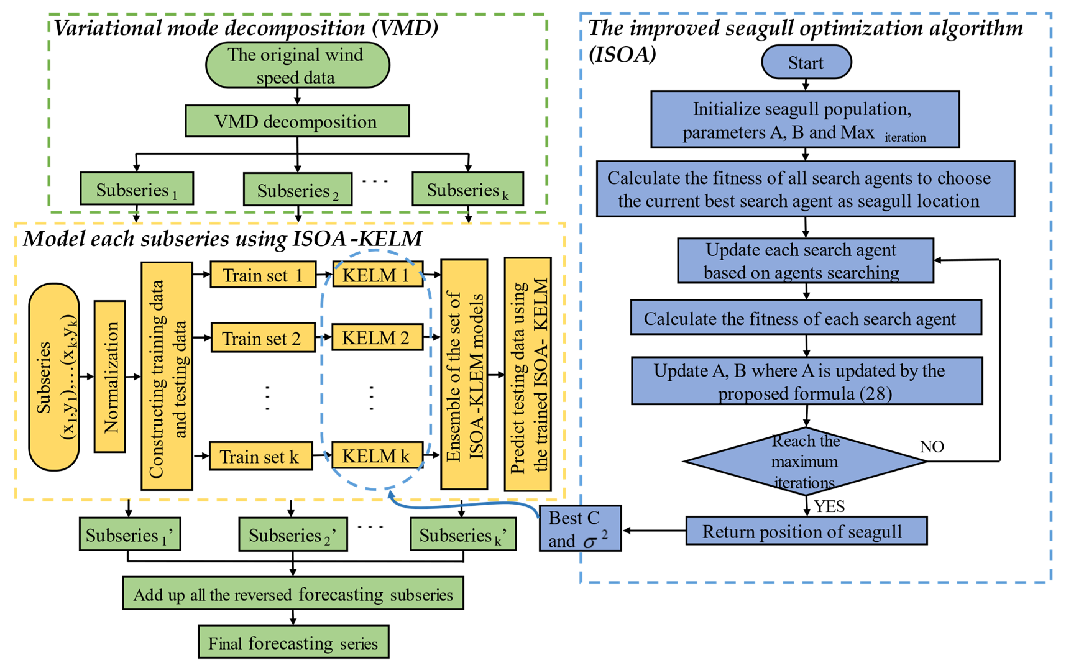
2.4. Workflow of the Hybrid Model

Through decomposition-based data preprocessing technology, VMD, SOA and KELM were combined to establish a hybrid method for wind speed prediction. To improve the prediction accuracy and search speed, an improved seagull algorithm was used to synchronously search the optimal parameters $C$ and ${\sigma }^2$ of KELM. The root mean square error was used as the fitness function. The workflow of this study is provided in Figure 1 and detailed explanations are given below.

2.4.1. Data Preprocessing

The original wind speed sequence was volatile and random. At this stage, VMD technology was used to decompose the complex wind speed data. The modes decomposed by VMD had their own center frequencies, which were stable relative to the original wind speed time series.

2.4.2. Hybrid Models Forecasting

The KELM model was used as the basic predictive model of the system because of its advantages of fast learning and a super-nonlinear description ability. The decomposed subseries were respectively predicted by the KELM model. ISOA was used to find the two best parameters of KELM at the same time in the subseries prediction process to ensure that the prediction of each subseries was optimal. The two parameters of each subseries reached the optimal value when the number of iterations reach the maximum. Then, the forecasting results of these models were combined together to obtain the final wind speed forecasting result. The ISOA-KELM process is shown in Figure 1.

2.4.3. Multi-Step ahead Forecasting

The developed combined model was employed in this study to forecasting short-term wind speed. One-step, two-step and three-step forecasts were included in this study. Multi-step forecasting was conducted to evaluate the predictive ability of the proposed strategy. The description of multi-step ahead forecasting is as follows: assume that the input datasets are $\left\{x(t-5),x(t-4),\cdots x(t-1),x(t)\right\}$ and the output datasets are $\left\{x(t+l)\right\}$, where $t$ donates a certain moment and $l$ donates the forecast horizon. When $l$ is equal to a positive integer, set the output data to $\widehat{y}(l)=x(t+l)$. At this time, $\widehat{y}(l)$ is the l-step ahead forecast value of the original $x(t+l)$.

3. Experimental Design

3.1. Data Description

The experimental data for this study were taken from the Shanghai (SH) wind farm, which possesses rich wind energy resources. These data sets were collected on 8 April, 4 July, 20 October and 15 January 2019. All data sets included 1006 points, which were recorded every 10 min and lasted approximately a week. The first six datasets were used for preheating, and the entire dataset was divided into a training set and a test set before the experiment. The first 80% was used for training, and the last 20% was used for testing. The maximum (Max.), minimum (Min.), mean, median (Med.), standard deviation (SD), kurtosis (Kurt.) and skewness (Skew) of the four data sets were also recorded, as shown in

Table 1. Statistical indicators of the four datasets.

Dataset	Period	Statistics Indicator
		Max. (m/s)	Min. (m/s)	Mean (m/s)	SD (m/s)	Skew.	Kurt.
Spring	8–14 April	15.17	0.37	6.97	2.79	0.19	2.31
Summer	4–10 July	21.39	0.12	7.36	4.32	1.27	4.14
Autumn	20–26 October	12.58	0.76	5.63	2.14	0.25	2.77
Winter	15–21 January	12.34	0.93	6.45	1.97	−0.11	3.07

.

3.2. Performance Metrics

The value predicted by the model often had an error with regard to the true value. The performance indicator evaluates the prediction effect of different models by evaluating the error between the observed value and the predicted value. Different evaluation indicators have different evaluation capabilities. In this study, the mean absolute error (MAE), root mean square error (RMSE) and mean absolute percentage error (MAPE) were calculated. The calculation methods of MAE and RMSE offset the positive and negative prediction errors, taking into account the average degree of error between the predicted value and the observed value. MAPE is the average value of absolute error and is the most widely implemented indicator used to reflect the effectiveness and reliability of aproposed new model. To explain the performance indicators more clearly,

Table 2. Three error metrics.

Metrics	Definition	Equation
MAE	Mean absolute error	$MAE=\frac{1}{N}{\displaystyle \sum _{i=1}^N\left|Y_o(i)-{\widehat{Y}}_p(i)\right|}$
RMSE	Root-mean-square error	$RMSE=\sqrt{\frac{1}{N}{\displaystyle \sum _{i=1}^N{\left(Y_o(i)-{\widehat{Y}}_p(i)\right)}^2}}$
MAPE	Absolute percentage error	$MAPE=\frac{1}{N}{\displaystyle \sum _{i=1}^N\left|\frac{Y_o(i)-{\widehat{Y}}_p(i)}{Y_o(i)}\right|}\times 100\%$

lists the definitions and specific formulas of the four error indicators. Here $Y_o(i)$ and ${\widehat{Y}}_p(i)$ represent the actual value and the predicted value, respectively, and $N$ is the sample size.

4. Different Experiments and Relative Analysis

In this section, a detailed evaluation and analysis of the proposed model are carried out. Two sets of experiments are designed, and the graphs and tables visually show the corresponding prediction results and evaluation indicators. The experimental setup and results are as follows.

4.1. Experimental Setup

Two sets of comparative experiments were used to compare the forecasting ability between the proposed model and other comparable models. Experiment 1 compared the proposed combined model with five independent models to investigate its prediction performance. Experiment 2 compared the forecasting accuracy between the proposed model and models using various data preprocessing technologies. The four data sets were tested by all models. The results of multistep ahead forecasting further illustrated the forecasting capability of different models. Three error evaluation indicators were used to quantify the predictive ability. The smaller the value of error criteria, the better the predictive performance.

In Experiment 1, we selected five widely used individual models (BP, SVM, LSTM, ELM and KELM) as the control group of the comparative experiment. In order to compare the developed strategy with the prediction ability based on different data preprocessing technologies, such as discrete wavelet transform (DWT), EMD and complementary ensemble empirical mode decomposition (CEEMD), we conducted experiment 2.

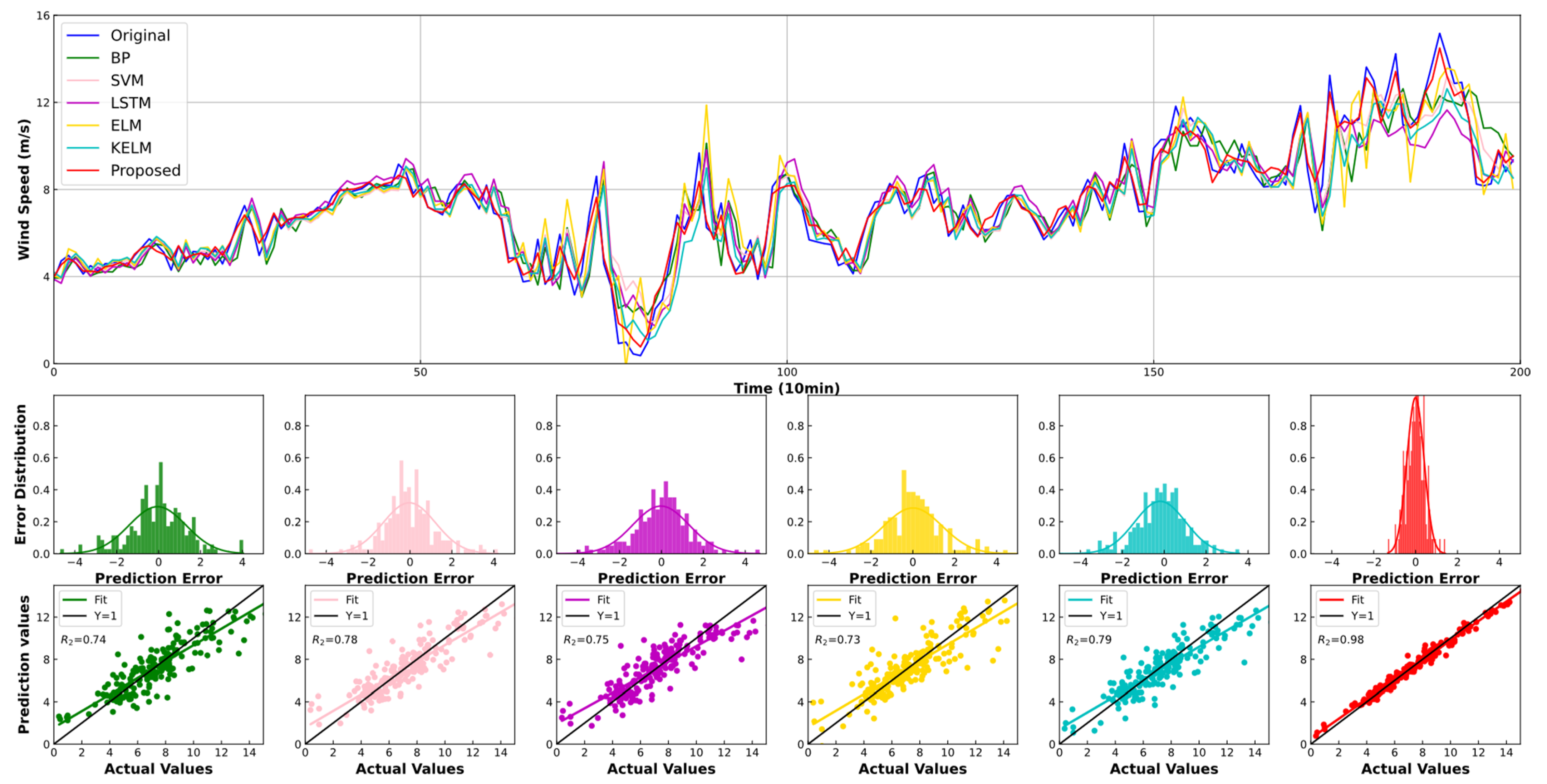
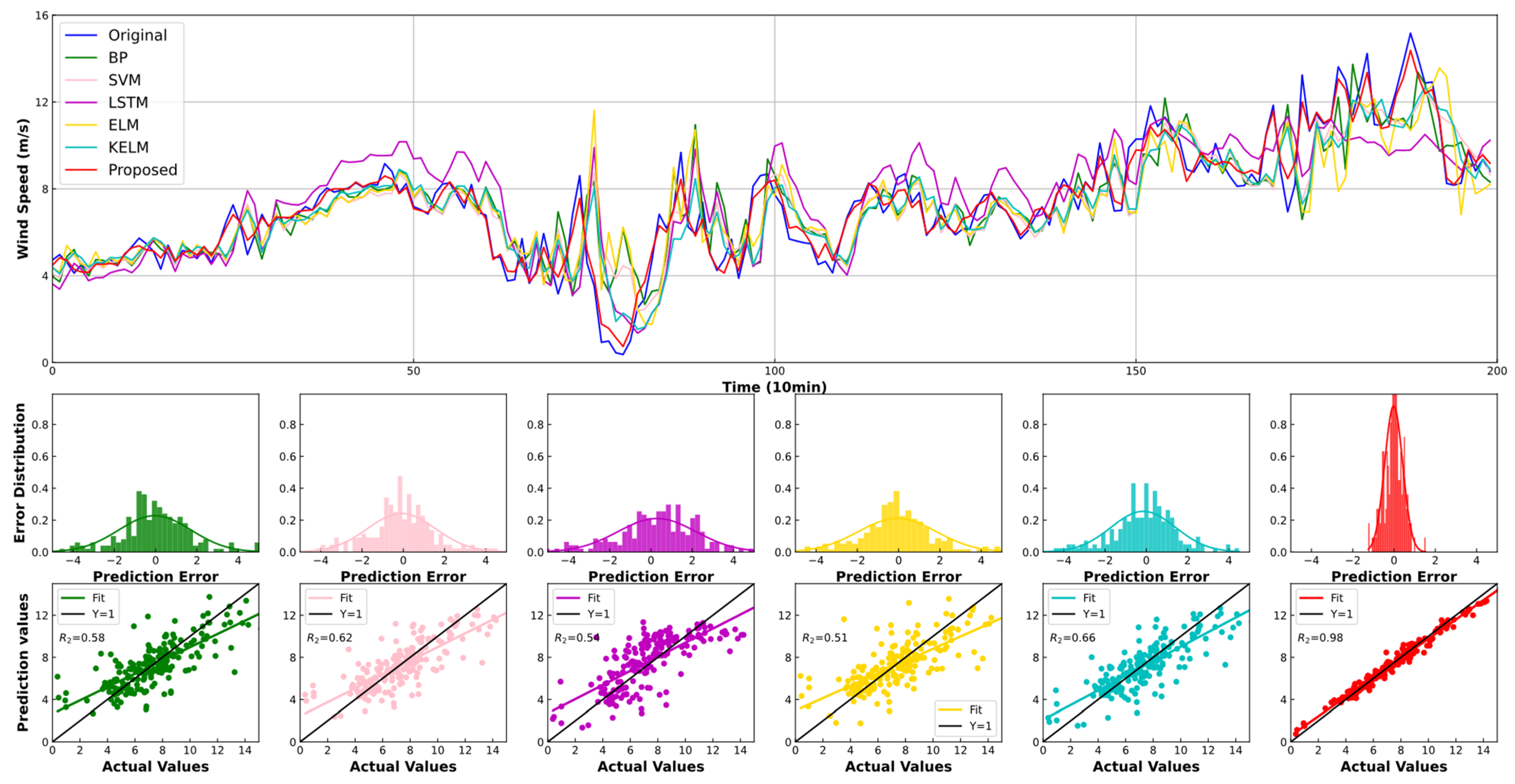
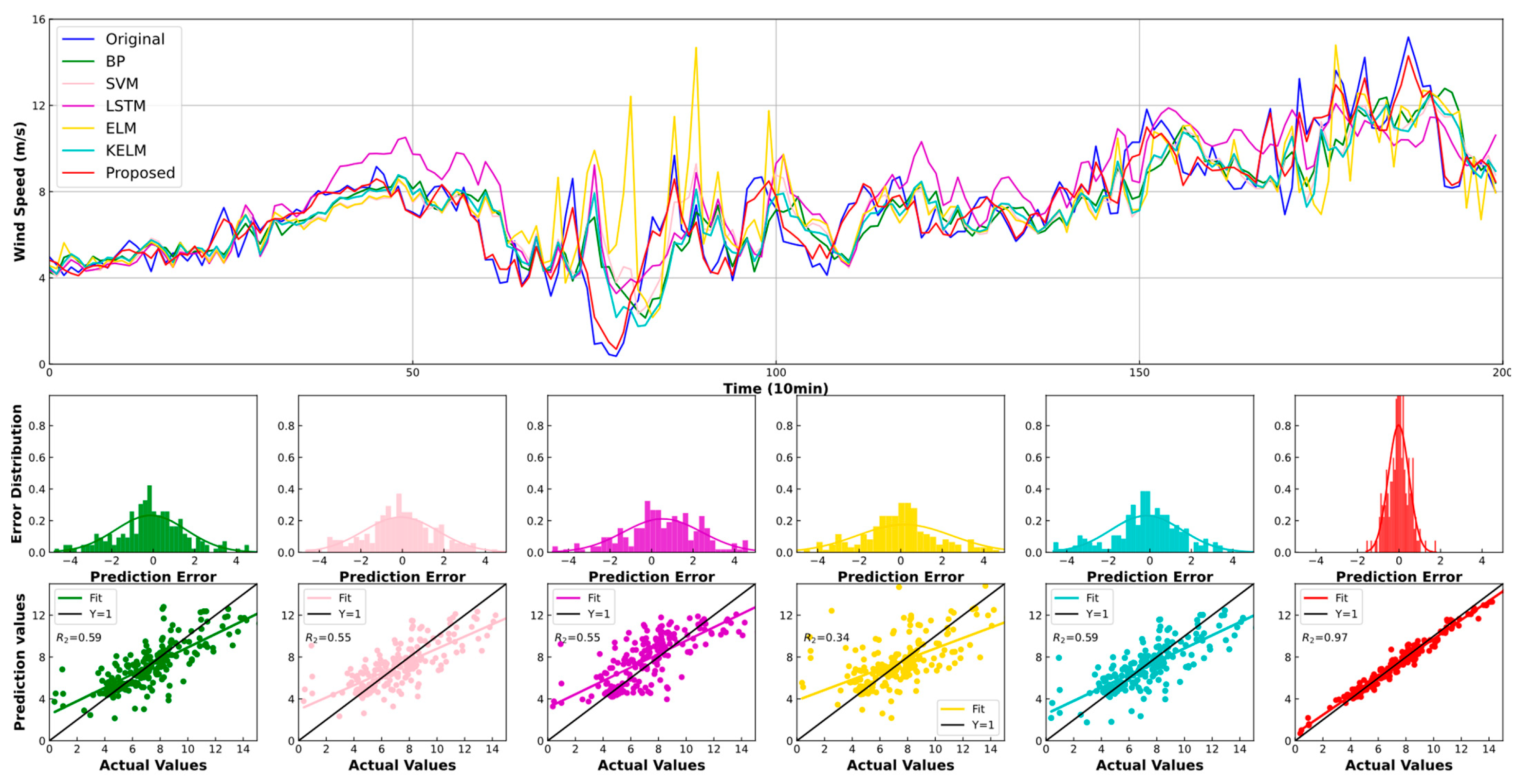
4.2. Experiment I: Comparison with Other Individual Models

Table 3. Comparison of forecasting performances of the proposed model and other independent models. BP: backpropagation; SVM: support vector machine; LSTM: long short-term memory; ELM: extreme learning machine; KELM: kernel extreme learning machine.

Datasets	Models	One-Step			Two-Step			Three-Step
		MAE	RMSE	MAPE	MAE	RMSE	MAPE	MAE	RMSE	MAPE
		(m/s)	(m/s)	(%)	(m/s)	(m/s)	(%)	(m/s)	(m/s)	(%)
SH Apr	BP	1.247	1.642	30.167	1.273	1.747	33.836	1.274	1.713	31.622
	SVM	0.919	1.248	23.690	1.202	1.648	31.104	1.338	1.796	35.701
	LSTM	1.014	1.331	21.583	1.496	1.919	29.888	1.516	1.961	36.335
	ELM	0.954	1.303	21.051	1.340	1.890	35.802	1.576	2.281	46.062
	KELM	0.888	1.190	17.373	1.156	1.568	23.916	1.270	1.731	29.056
	Proposed	0.315	0.408	6.606	0.330	0.436	6.837	0.378	0.496	7.512
SH Jul	BP	0.677	0.864	9.792	0.770	0.961	11.105	1.002	1.228	14.638
	SVM	0.519	0.678	7.434	0.687	0.858	9.956	0.767	0.931	11.197
	LSTM	0.638	0.819	8.561	0.761	0.946	11.168	0.765	0.952	10.830
	ELM	0.521	0.684	7.355	0.693	0.856	9.931	0.787	0.969	11.431
	KELM	0.515	0.672	7.342	0.680	0.839	9.883	0.739	0.900	10.853
	Proposed	0.221	0.270	3.140	0.226	0.276	3.205	0.237	0.288	3.361
SH Oct	BP	0.676	0.886	8.966	1.055	1.326	13.731	0.853	1.120	11.471
	SVM	0.749	1.079	8.763	0.937	1.243	11.468	1.070	1.393	13.285
	LSTM	0.616	0.823	7.731	0.823	1.073	10.557	0.937	1.221	11.753
	ELM	0.671	0.947	8.184	0.897	1.219	11.145	1.045	1.396	12.996
	KELM	0.750	1.018	8.981	0.941	1.210	11.672	1.056	1.348	13.268
	Proposed	0.182	0.235	2.367	0.198	0.257	2.541	0.223	0.287	2.844
SH Jan	BP	0.809	1.095	11.848	0.880	1.179	13.159	0.985	1.347	14.676
	SVM	0.629	0.903	9.066	0.828	1.112	12.333	0.942	1.262	14.244
	LSTM	0.655	0.940	9.485	0.875	1.161	12.714	0.902	1.223	13.556
	ELM	0.739	1.120	10.279	0.970	1.374	14.066	1.092	1.539	15.869
	KELM	0.632	0.891	9.179	0.823	1.104	12.239	0.916	1.239	13.783
	Proposed	0.252	0.333	3.894	0.280	0.372	4.276	0.314	0.418	4.737

shows the comparison of the results of the proposed model and the other individual models in the four seasons datasets. Figure 2, Figure 3 and Figure 4 show the forecasting results of individual forecasting models in SH in April. At the top of the chart, the predicted results versus 10 min interval sampling points for all forecasting models are shown. Below, the error distribution diagram of forecasting and the scatter diagram of each individual model are presented.

For SH Apr, in the one-step forecasting, the proposed model showed the best MAE, RMSE and MAPE scores at 0.315, 0.408 and 6.606% respectively, followed by the KELM model, whose values for MAE, RMSE and MAPE were 0.888, 1.190 and 17.373% respectively. The worst was the BP neural network, with MAE, RMSE and MAPE scores of 1.247, 1.642 and 30.167%, respectively. When the model forecasting was two-step, the developed model had the best accuracy with an RMSE of 0.436. In the three-step, the proposed model still had the best predictive ability with an RMSE of 0.496, but the second most accurate model was the BP network. Figure 4, Figure 5 and Figure 6 shows the prediction results of the proposed model and the individual model in the spring experimental series (SH Apr).

For SH July, when the forecasting is one-step, the proposed VMD-ISOA-KELM hybrid model achieves the highest accuracy with a MAPE value of 3.140%. Comparatively, the individual models have fairly lower MAPE values of 9.792%, 7.434%, 8.561%, 7.355% and 7.342%, respectively. In the two-step and three-step forecasting, the developed combined model is more effective than the other methods for wind speed forecasting. Meanwhile, KELM has the lowest MAPE values at 7.342% and 9.883% in the one-step and two-step among the remaining four individual models.

For SH Oct, according to the evaluation criteria shown in Table 3, the proposed model still outperformed the individual models in the three steps, with MAPE values of 2.367%, 2.541% and 2.844%. According to the obtained MAPE, long short-term memory (LSTM) is ranked as the second most effective model in the three forecasts, with lower MAPE values of 7.731%, 10.557% and 11.753%.

For SH Jan, in all forecasting steps, the developed combined model exceeded the five benchmark models with MAPE values of 3.894%, 4.276% and 4.737%. In the two-step and three-step forecasting, the five individual models performed poorly, and their RMSE values were all over 1.

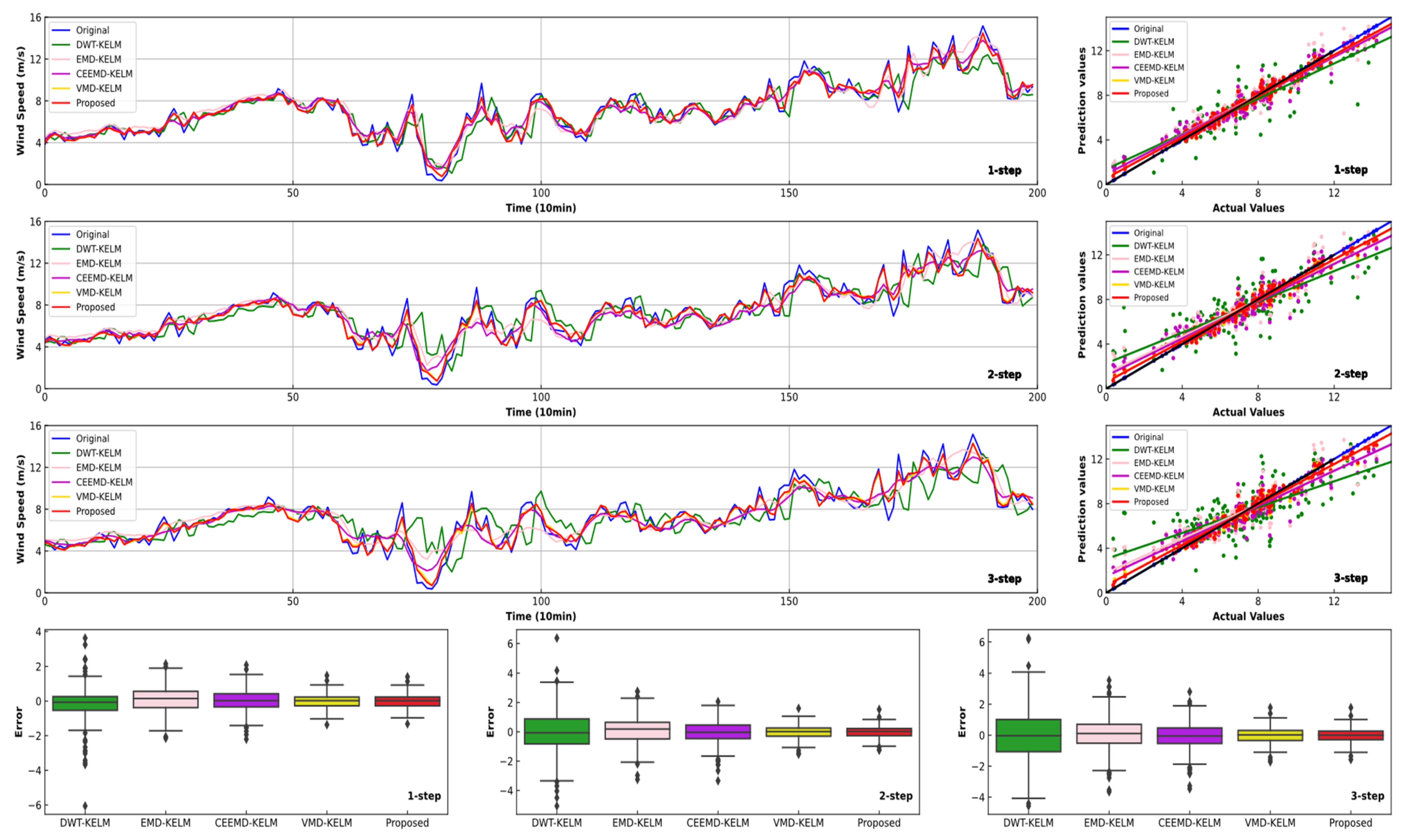
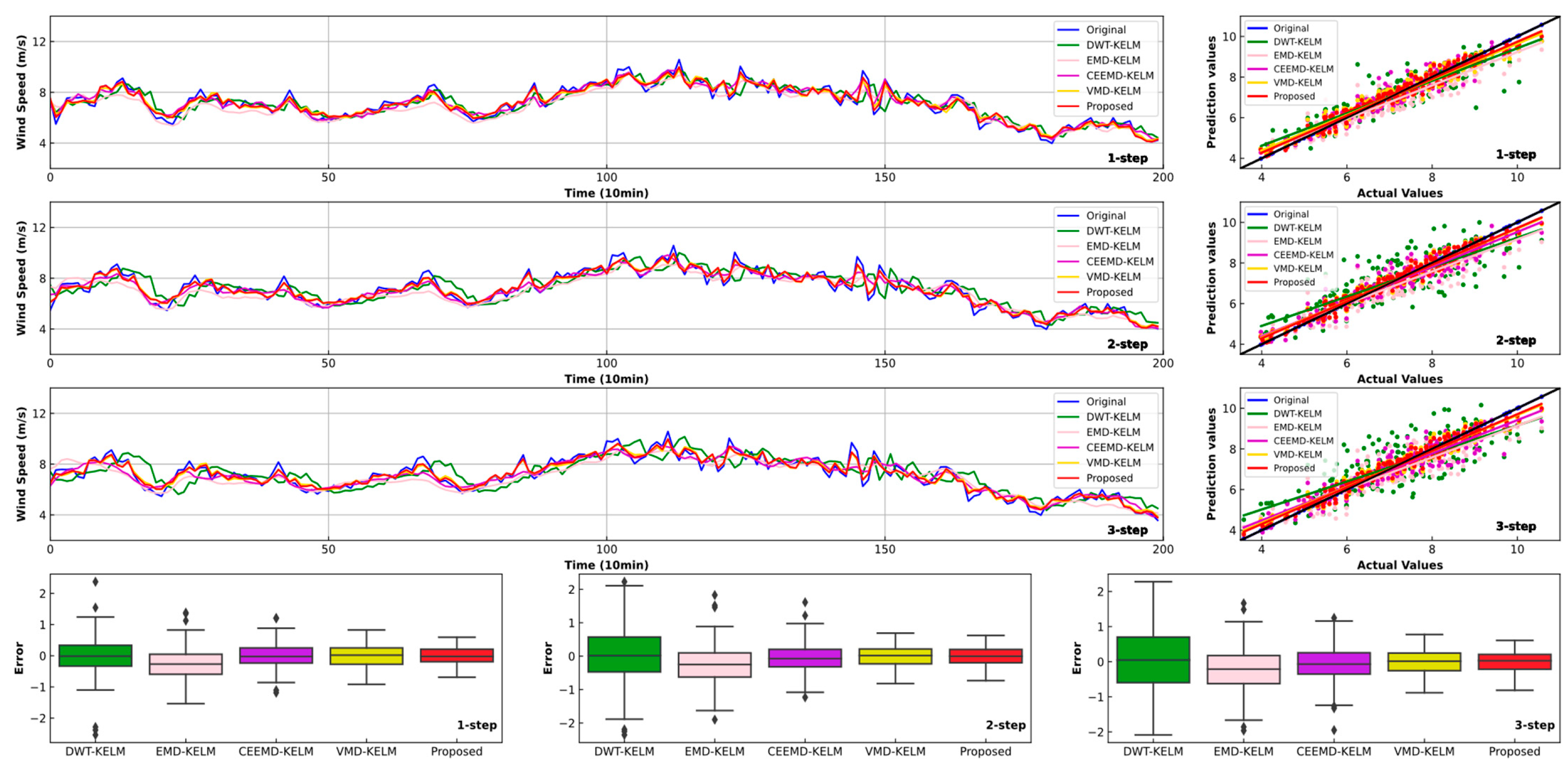
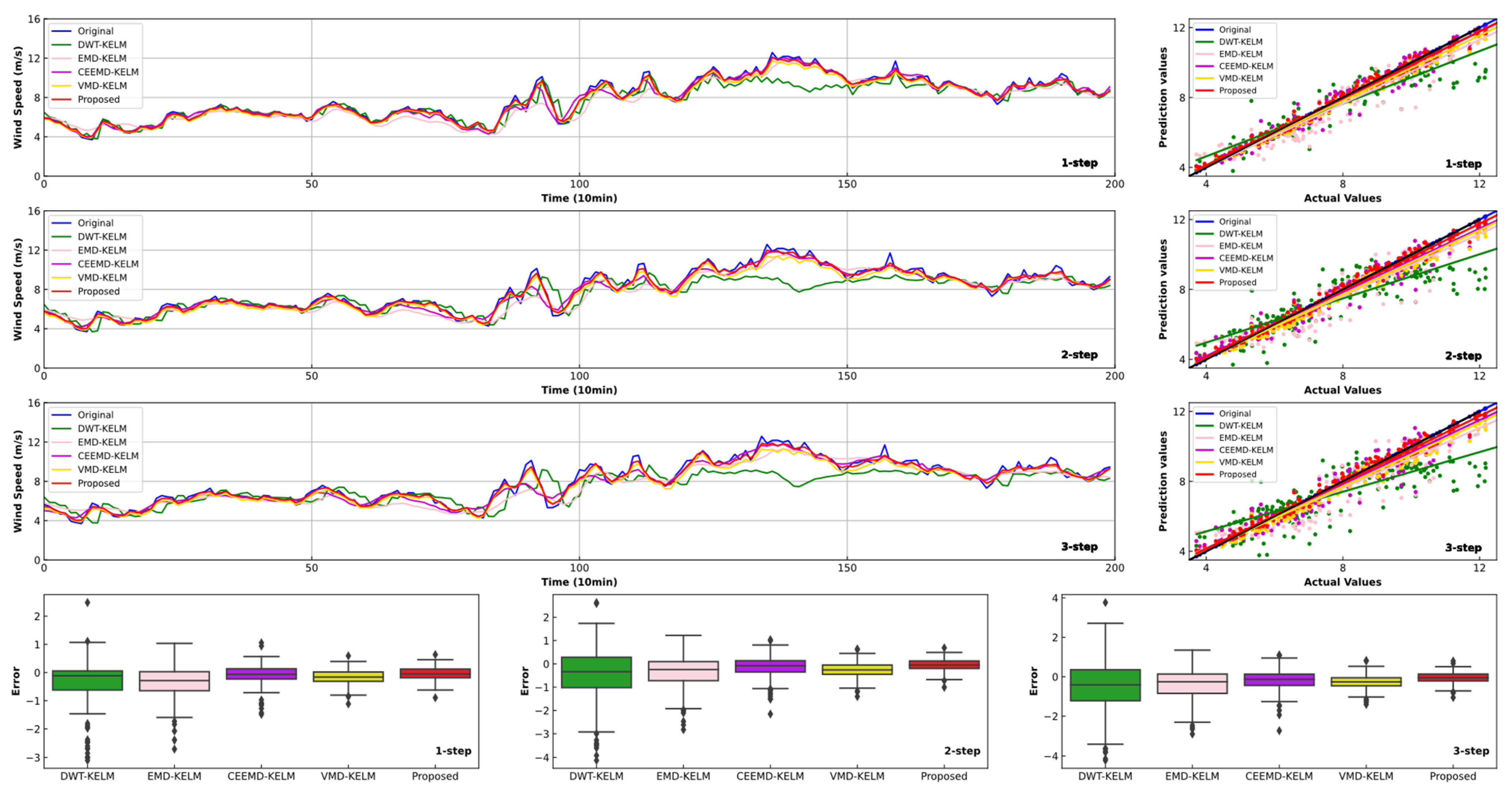
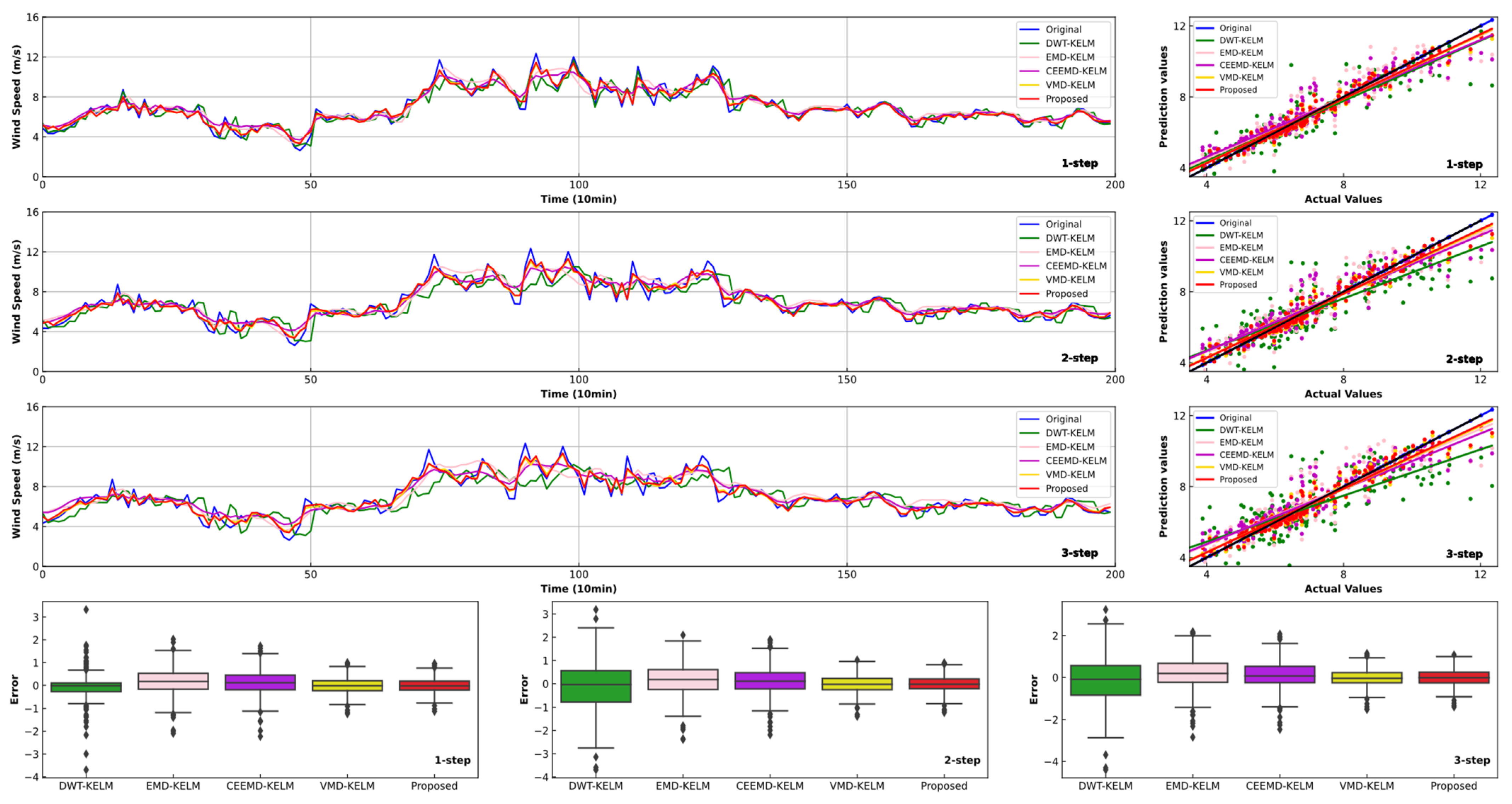
4.3. Experiment II: Comparsion with Other Models Using Different Data Preprocessing Methods

This experiment demonstrated the forecasting performance of the wind speed time series by comparing the VMD-ISOA-model with models using different data preprocessing methods, namely DWT, EMD and CEEMD. The comparison results are listed in

Table 4. Comparison of forecasting performances of the combined model and other models using different data preprocessing methods. DWT: discrete wavelet transform; EMD: empirical mode decomposition; CEEMD: complementary ensemble empirical mode decomposition; VMD: variational mode decomposition.

Datasets	Models	One-Step			Two-Step			Three-Step
		MAE	RMSE	MAPE	MAE	RMSE	MAPE	MAE	RMSE	MAPE
		(m/s)	(m/s)	(%)	(m/s)	(m/s)	(%)	(m/s)	(m/s)	(%)
SH Apr	DWT	0.639	1.074	18.12	1.121	1.532	28.585	1.377	1.808	36.064
	EMD	0.606	0.768	13.779	0.764	0.999	19.892	0.856	1.156	23.910
	CEEMD	0.552	0.731	14.308	0.634	0.860	14.796	0.699	0.951	16.466
	VMD	0.331	0.437	7.089	0.353	0.471	7.412	0.404	0.528	8.340
	Proposed	0.315	0.408	6.606	0.330	0.436	6.837	0.378	0.496	7.512
SH Jul	DWT	0.427	0.589	6.116	0.649	0.825	9.301	0.759	0.917	11.002
	EMD	0.441	0.555	6.031	0.494	0.630	6.817	0.531	0.671	7.346
	CEEMD	0.288	0.374	4.114	0.334	0.436	4.682	0.388	0.503	5.464
	VMD	0.289	0.353	4.098	0.248	0.302	3.533	0.279	0.340	4.002
	Proposed	0.221	0.270	3.140	0.226	0.276	3.205	0.237	0.288	3.361
SH Oct	DWT	0.521	0.848	5.981	0.875	1.206	10.587	1.043	1.388	12.927
	EMD	0.505	0.677	6.744	0.565	0.768	7.452	0.635	0.844	8.293
	CEEMD	0.266	0.372	3.452	0.350	0.485	4.559	0.410	0.561	5.412
	VMD	0.251	0.316	3.114	0.337	0.423	4.154	0.365	0.458	4.529
	Proposed	0.182	0.235	2.367	0.198	0.257	2.541	0.223	0.287	2.844
SH Jan	DWT	0.416	0.701	6.016	0.780	1.042	11.552	0.917	1.216	13.738
	EMD	0.51	0.672	7.569	0.579	0.764	8.661	0.634	0.838	9.448
	CEEMD	0.442	0.596	6.807	0.489	0.669	7.610	0.531	0.727	8.246
	VMD	0.273	0.364	4.200	0.308	0.410	4.690	0.336	0.445	5.077
	Proposed	0.252	0.333	3.894	0.280	0.372	4.276	0.314	0.418	4.737

and Figure 5, Figure 6, Figure 7 and Figure 8. More details of the experiment are given below:

For SH Apr, in the one-step forecasting, the proposed model showed the best performance with a MAPE value of 6.606%. In comparison, the model after pretreatment of VMD ranked as the second most effective model among the other data preprocessing technologies, with MAPE values of 7.089%, 7.412% and 8.340%, respectively, from one-step to three-step forecasting. Correspondingly, the DWT-Model showed the worst forecasting accuracy with MAPE values of 18.12%, 28.585%, and 36.064% from one-step to three-step forecasting.

For SH July, according to the evaluation criteria shown in Table 4, the proposed model still outperformed the individual models in one-step forecasting, with the lowest MAE, RMSE and MAPE values of 0.221, 0.270 and 3.140%. According to the obtained MAPE, LSTM ranked as the second most effective model in the three forecasting, with lower MAPE values of 7.731%, 10.557% and 11.753%.

For SH Oct, when the forecasting was one-step, the proposed VMD-ISOA-KELM hybrid model achieved the highest accuracy with a MAPE value of 3.140%. Comparatively, the DWT-Model, EMD-Model, CEEMD-Model and VMD-Model had MAPE values of 5.981%, 6.744%, 3.452%, 7.355% and 7.342%, respectively, which wereinferior to our developed hybrid model. The comparison results of our forecasting strategy and DWT-Model, EMD-Model and CEEMD-Model are shown in Figure 7.

For SH Jan, when the model forecasting is one-step, the prediction accuracy of the hybrid model, which has the lowest MAE, RMSE and MAPE values of 0.252, 0.333 and 3.894% respectively, was still superior compared to the other models using different preprocessing methods. In addition, the CEEMD -Model showed a better forecasting performance than EMD, with MAPE values of 6.807%, 7.601% and 8.246% respectively when the model forecasting changed from one-step to three-step.

5. Discussion

This section presents an insightful discussion of the experiment results, namely the main contributions, the performance of the employed optimization algorithm, the effectiveness of the proposed model and improvements of the proposed model. The concrete details are as follows.

5.1. Main Achievements and Results

Considering the noisy and highly nonlinear features of real wind speed data, this paper mainly proposes an optimized hybrid forecasting strategy based on VMD, KELM and ISOA for short-term wind speed forecasting. VMD decomposition technology has advantages in terms of weakening the non-stationarity of wind speed data, which were found by comparing and analyzing the experimental results of VMD-KELM, EMD-KELM, CEEMD-KELM and DWT-KELM techniques. With regard to wind speed forecasting, KELM is used as a powerful regression core to characterize the relationship between the samples in each subsequence and the expected output. Experiment 1 showed that KELM has a certain advantage in several widely used individual models. However, the prediction accuracy of KELM is sensitive to parameters. For this purpose, a novel algorithm ISOA was proposed to solve optimization issues, transforming the global optimization strategy from linear to non-linear. In order to further improve the prediction, the two parameters of KELM were optimized by the proposed ISOA algorithm. The superiority of the proposed prediction strategy was shown through relative experiments and contrastive analysis.

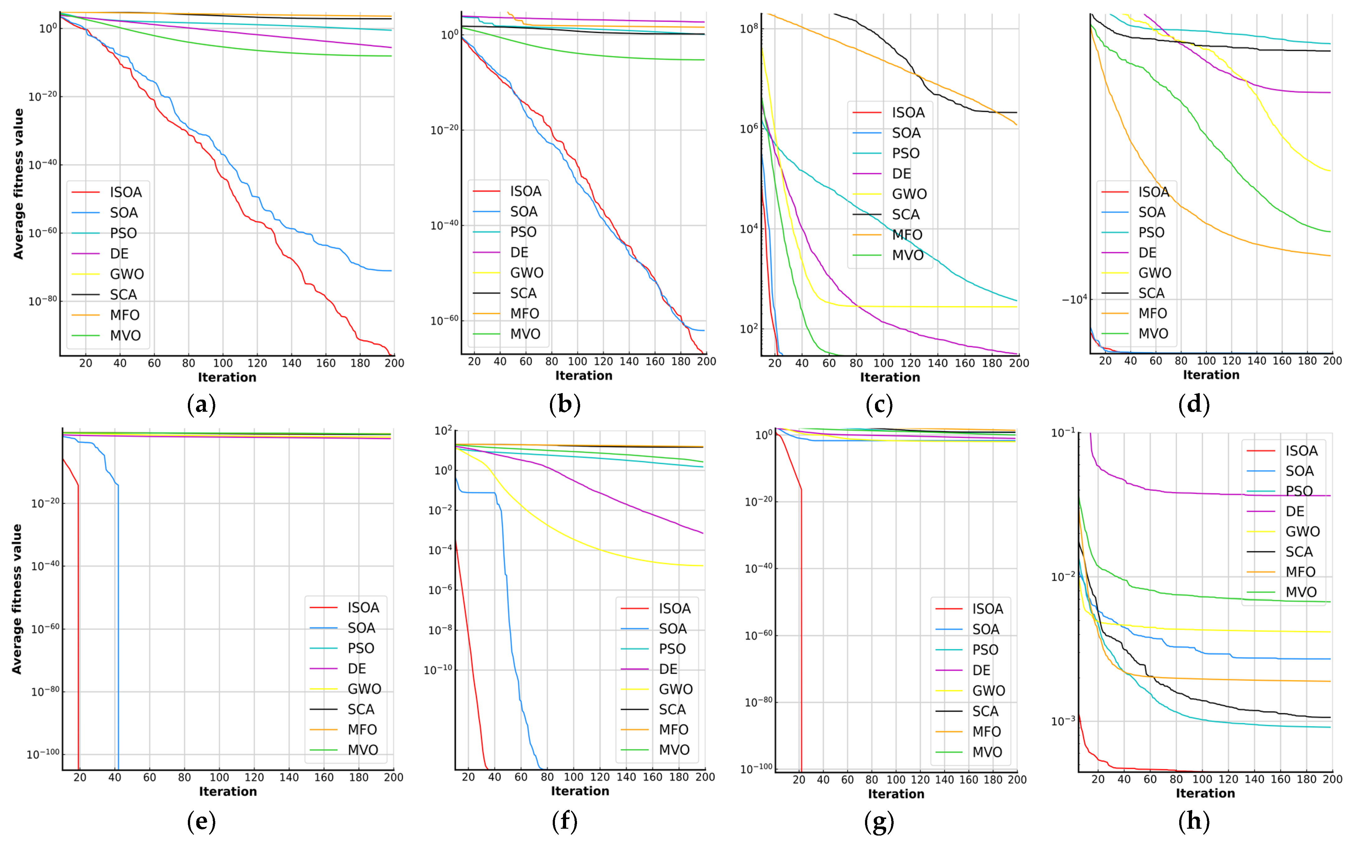
5.2. Performance of the Employed Optimization Algorithm

In this subsection, eight typical benchmark functions were used to measure and verify the proposed ISOA algorithm, including three unimodal functions and five multimodal functions. The unimodal function was used to test the development ability, and the multimodal function was used to test the development ability and avoid falling into the local optimum. These benchmark functions are shown in

Table 5. Description of unimodal, multimodal and fixed-dimension benchmark functions.

Function	Peak	Dim	Range	${\mathsf{f}}_{\min }$
$f_1={\displaystyle {\sum }_{i=1}^n{x}_i^2}$	Unimodal	30	[−100, 100]	0
$f_2={\displaystyle {\sum }_{i=1}^n\left|x_i\right|}+{\displaystyle \prod _{i=1}^n\left|x_i\right|}$	Unimodal	30	[−10, 10]	0
$f_5={\displaystyle {\sum }_{i=1}^n\left[100{\left(x_{i+1}-x_i^2\right)}^2+{\left(x_i-1\right)}^2\right]}$	Unimodal	30	[−30, 30]	0
$f_8={\displaystyle {\sum }_{i=1}^n-x_i\sin (\sqrt{\left|x_i\right|})}$	Multimodal	30	[−500, 500]	−12,569.5
$f_9={\displaystyle {\sum }_{i=1}^n\left[x_i^2-10\cos (2\pi x_i)+10\right]}$	Multimodal	30	[−5.12, 5.12]	0
$f_{10}=-20\exp \left(-0.2\sqrt{\frac{1}{n}{\displaystyle {\sum }_{i=1}^n{x}_i^2}}\right)-\exp \left(\frac{1}{n}{\displaystyle \sum _{i=1}^n\cos (2\pi x_i)}\right)+20+e$	Multimodal	30	[−32, 32]	0
$f_{11}=\frac{1}{4000}{\displaystyle {\sum }_{i=1}^n{x}_i^2}-{\displaystyle \prod _{i=1}^n\cos \left(\frac{x_i}{\sqrt{i}}\right)}+1$	Multimodal	30	[−600, 600]	0
$f_{15}={{\displaystyle {\sum }_{i=1}^{11}\left[a_i-\frac{x_1\left(b_i^2+b_i{z}_2\right)}{b_i^2+b_i{z}_3+z_4}\right]}}^2$	Fixed-dimension	4	[−5, 5]	0.0003

. Peak donates the features of the function, Dim donates the dimension of the function, Range donates the definition domain of the function and $f_{\min }$ donates the optimal value of the function.

In addition, seven classic optimization algorithms were selected for comparison with the new algorithm, namely particle swarm optimization (PSO), differential evolution (DE), seagull optimization algorithm (SOA), gray wolf optimizer (GWO), sine cosine algorithm (SCA), moth flame optimization (MFO) and the multiverse optimizer (MVO). All algorithms were run 50 times on each benchmark function and with a maximum of 200 iterations. Figure 9 shows the convergence curve of ISOA and other comparison algorithms with the same dimensions. Compared with SOA, ISOA was closer to the optimal value with the same number of iterations. Among all comparative functions, ISOA had the fastest convergence speed, reflecting ISOA’s efficient exploration capability. In order to measure the experimental results, the average value (AVG) and standard deviation (STD) were used to evaluate the results. Note that the best results are presented in bold. The data in

Table 6. Test results of 50 trials of ISOA and other algorithms.

ID	Metric	ISOA	SOA	PSO	DE	GWO	SCA	MFO	MVO
F1	AVG	1.80 × 10−96	9.18 × 10−72	3.90 × 10−1	2.64 × 10−6	8.70 × 10−9	6.87 × 102	3.98 × 104	8.41 × 100
	STD	1.27 × 10−95	6.49 × 10−71	2.75 × 10−1	2.15 × 10−6	8.14 × 10−9	7.40 × 102	5.13 × 103	2.60 × 100
F2	AVG	9.45 × 10−68	9.40 × 10−63	1.23 × 100	1.05 × 10−4	5.61 × 10−6	1.50 × 100	3.95 × 101	4.28 × 101
	STD	4.51 × 10−67	3.97 × 10−62	4.62 × 10−1	3.42 × 10−5	2.91 × 10−6	1.41 × 100	1.90 × 101	8.35 × 101
F5	AVG	2.88 × 101	2.88 × 101	4.17 × 102	3.17 × 101	2.78 × 102	2.05 × 106	5.54 × 106	1.07 × 103
	STD	2.95 × 10−2	4.62 × 10−2	5.17 × 102	1.84 × 101	7.76 × 101	4.70 × 106	1.91 × 107	1.59 × 103
F8	AVG	−1.25 × 104	−1.25 × 104	−3.40 × 103	−4.18 × 103	−5.81 × 103	−3.51 × 103	−8.31 × 103	−7.51 × 103
	STD	5.07 × 101	7.95 × 101	5.23 × 102	3.57 × 101	1.16 × 103	2.71 × 102	8.04 × 102	5.74 × 102
F9	AVG	0.00 × 100	0.00 × 100	1.08 × 102	4.72 × 100	1.47 × 101	1.03 × 102	1.73 × 102	1.35 × 102
	STD	0.00 × 100	0.00 × 100	3.25 × 101	2.11 × 100	8.63 × 100	4.94 × 101	2.72 × 101	3.23 × 101
F10	AVG	8.89 × 10−16	8.89 × 10−16	1.51 × 100	7.09 × 10−4	1.67 × 10−6	1.47 × 101	1.57 × 101	2.70 × 100
	STD	0.00 × 100	0.00 × 100	5.16 × 10−1	3.08 × 10−4	9.73 × 10−6	7.21 × 100	4.69 × 100	5.79 × 10−1
F11	AVG	0.00 × 100	2.02 × 10−2	5.96 × 100	9.69 × 10−2	1.03 × 10−2	6.89 × 100	2.55 × 101	1.07 × 100
	STD	0.00 × 100	1.43 × 10−1	3.09 × 100	5.57 × 10−2	1.48 × 10−2	5.44 × 100	3.35 × 101	1.98 × 10−2
F15	AVG	3.70 × 10−4	4.40 × 10−3	9.10 × 10−4	3.67 × 10−2	4.20 × 10−3	1.10 × 10−3	1.90 × 10−3	6.70 × 10−3
	STD	2.90 × 10−4	4.80 × 10−3	2.19 × 104	4.24 × 10−2	7.71 × 10−3	3.96 × 10−4	4.00 × 10−3	8.81 × 10−3

demonstrate that the optimization result of ISOA was the best among all optimization algorithms. At the same time, the STD values of the solutions were still the smallest, indicating the stability of the ISOA.

5.3. Effectiveness of the Developed Strategy

To investigate the different effectiveness of the developed model and other comparison models, the Diebold-Mariano (DM) test was employed, which is a statistical hypothesis test. The null hypothesis $H_0$ and alternative hypothesis $H_1$ are written as follows:

$$H_0:E\left[F\left(e_i^1\right)\right]=E\left[F\left(e_i^2\right)\right]$$

(29)

$$H_1:E\left[F\left(e_i^1\right)\right]\ne E\left[F\left(e_i^2\right)\right]$$

(30)

where $F$ is the loss function of forecasting errors, $e_i^1$ and $e_i^2$ are forecasting errors between actual values and forecasted values of the different forecasting models. Then, implementing statistical reasoning by DM test statistics, the DM test statistic values can be computed by

$$DM=\frac{{\displaystyle {\sum }_{i=1}^n\left(F(e_i^1)-F(e_i^2)\right)}/n}{\sqrt{{\tau }^2/n}}{\tau }^2$$

(31)

where ${\tau }^2$ denotes the estimation for the variance of $F(e_i^1)-F(e_i^2)$.

Table 7. Diebold–Mariano (DM) test of different models.

Model	1-Step	2-Step	3-Step
BP	7.9252	8.6438	8.6631
SVM	6.3969	7.9864	8.4509
LSTM	7.0239	8.2106	8.6123
ELM	6.9602	7.0022	7.3714
KELM	6.6534	8.1960	8.7345
DWT	6.3367	6.6578	7.5850
EMD	4.2412	6.6594	6.8246
CEEMD	5.5755	5.4812	5.6415
VMD	3.6386	4.6848	4.1407

lists the mean DM values from one- to three-step forecasting. Regardless of the DM values for one-step, two-step and three-step forecasting, the DM values of the nine comparison models were all obviously significant. For some classic individual models, all DM values were much larger than the upper limits at a 1% significance level. Moreover, when comparing with models applying different data pretreatment technologies, the proposed hybrid model similarly obtains showed a improvement.

5.4. Improvements of the Proposed Model

To further discuss and evaluate the degree of improvement in forecasting when comparing a selected model with the proposed mode, we adopted an improvement percentage of the MAPE criteria ($P_{MAPE}$), which enabled a comprehensive analysis of the proposed hybrid model. It is defined as

$$P_{\mathrm{MAPE}}=\left|\frac{{\mathrm{MAPE}}_1{-\mathrm{MAPE}}_2}{{\mathrm{MAPE}}_1}\right|\times 100\%$$

(32)

According to the definition of $P_{\mathrm{MAPE}}$, the larger the $P_{\mathrm{MAPE}}$, the better the forecasting accuracy of our developed model relative to the selected models.

Table 8. Improvement percentages of the proposed model.

Model	SH April			SH July			SH October			SH January
	1-Step	2-Step	3-Step	1-Step	2-Step	3-Step	1-Step	2-Step	3-Step	1-Step	2-Step	3-Step
BP	78.10	79.79	76.24	67.93	71.14	77.04	73.60	81.49	75.21	67.13	67.51	67.72
SVM	72.11	78.02	78.96	57.76	67.81	69.98	72.99	77.84	78.59	57.05	65.33	66.74
LSTM	69.39	77.12	79.33	63.32	71.30	68.97	69.38	75.93	75.80	58.95	66.37	65.06
ELM	68.62	80.90	83.69	57.31	67.73	70.60	71.08	77.20	78.12	62.12	69.60	70.15
KELM	61.98	71.41	74.15	57.23	67.57	69.03	73.64	78.23	78.56	57.58	65.06	65.63
DWT	63.54	76.08	79.17	48.66	65.54	69.45	60.42	76.00	78.00	35.27	62.98	65.52
EMD	52.06	65.63	68.58	47.94	52.99	54.25	64.90	65.90	65.71	48.55	50.63	49.86
CEEMD	53.83	53.79	54.38	23.68	31.55	38.49	31.43	44.26	47.45	42.79	43.81	42.55
VMD	6.81	7.76	9.93	23.38	9.28	16.02	23.99	38.83	37.20	7.29	8.83	6.70

Note: The units of all values revealed in the table are (%).

presents the improvement percentages of MAPE for the proposed model and other forecasting models. From further analysis of the results shown in Table 8, we are able to state the following.

• The improvement ratios of the evaluation indicators of the proposed strategy compared with individual models are greater than 50%. Among the classic individual models, the maximum improvement percentages of MAPE for the three steps forecasting are 78.01% (SH Apr, one-step), 81.49% (SH Oct, two-step) and 83.69% (SH Jan, three-step), which shows the developed model’s significant improvements to multi-step forecasting.
• Similar to previous research, when compared with other models using different data preprocessing technologies, the improvements in the forecasting effectiveness of the proposed model are fairly evident. For instance, in comparison with DWT-KELM, EMD-KELM, CEEMD-KELM and VMD-KELM, the proposed model leads to 63.54%, 52.06%, 53.83% and 6.81% reductions for one-step forecasting, respectively. Thus, the developed combined model can obtain satisfactory forecasting effectiveness.
• These results show that there is still much room for individual models to improve forecasting accuracy. Adding a data preprocessing technique can significantly improve the forecast precision. However, the use of optimization algorithms can further improve the accuracy and stability of short-term wind speed forecasting.

6. Conclusions

To follow the trend of clean energy development, strive to achieve low-carbon environmental protection, and vigorously develop wind energy resources, this paper proposes a hybrid forecasting model based on VMD, an improved seagull optimization algorithm and KELM. Firstly, VMD is applied to decompose the given non-stationary wind speed data into several subseries with various scales. Then, KELM is used as a powerful regression core to characterize the relationship between the samples in each subsequence and the expected output. To enhance the prediction performance, the proposed ISOA is designed by including a nonlinear formula, which controls the population migration process and attack process of SOA. Subsequently, the proposed ISOA algorithm is applied to the simultaneous optimization of two parameters in the KELM model. Finally, the final predicted value is obtained by summing the results of all subseries. Furthermore, to evaluate the effectiveness and applicability of the developed combined model, different forecasting models are implemented on four datasets. The selected forecasting models includes five classic individual models and four hybrid models. The experimental results of the three metrics show that (1) the VMD is effective in improving the accuracy and stability of the wind speed predictions; (2) compared with the common ANN and SVM models, the KELM models show advantages in capturing the nonlinear characteristics of the wind speed time series; (3) regardless of the forecasting step or the observation datasets, the proposed combined strategy was superior to all of the selected methods with average MAPE values of 3.865%, 4.213% and 4.614% for one- to three-step forecasting.

References

1. Anoune, K.; Bouya, M.; Astito, A.; Abdellah, A.B. Sizing methods and optimization techniques for PV-wind based hybrid renewable energy system: A review. Renew. Sustain. Energy Rev. 2018, 93, 652–673. [Google Scholar] [CrossRef]
2. Duan, J.; Zuo, H.; Bai, Y.; Duan, J.; Chang, M.; Chen, B. Short-term wind speed forecasting using recurrent neural networks with error correction. Energy 2021, 217, 119397. [Google Scholar] [CrossRef]
3. Lee, J.; Zhao, F.; Dutton, A.; Lathigara, A. Global wind Report 2019; Global Wind Energy Council (GWEC): Brussels, Belgium, 2020; Available online: https://gwec.net/global-wind-report-2019/ (accessed on 25 March 2020).
4. Jiang, P.; Liu, Z.; Niu, X.; Zhang, L. A combined forecasting system based on statistical method, artificial neural networks, and deep learning methods for short-term wind speed forecasting. Energy 2020, 217, 119361. [Google Scholar] [CrossRef]
5. Peng, T.; Zhang, C.; Zhou, J.; Nazir, M.S. Negative correlation learning-based RELM ensemble model integrated with OVMD for multi-step ahead wind speed forecasting. Renew. Energy 2020, 156, 804–819. [Google Scholar] [CrossRef]
6. Song, J.; Wang, J.; Lu, H. A novel combined model based on advanced optimization algorithm for short-term wind speed forecasting. Appl. Energy 2018, 215, 643–658. [Google Scholar] [CrossRef]
7. Landberg, L. Short-term prediction of the power production from wind farms. J. Wind. Eng. Ind. Aerodyn. 1999, 80, 207–220. [Google Scholar] [CrossRef]
8. Salcedo-Sanz, S.; Perez-Bellido, Á.M.; Ortiz-García, E.G.; Portilla-Figueras, A.; Prieto, L.; Correoso, F. Accurate short-term wind speed prediction by exploiting diversity in input data using banks of artificial neural networks. Neurocomputing 2009, 72, 1336–1341. [Google Scholar] [CrossRef]
9. Prósper, M.A.; Otero-Casal, C.; Fernández, F.C.; Miguez-Macho, G. Wind power forecasting for a real onshore wind farm on complex terrain using WRF high resolution simulations. Renew. Energy 2019, 135, 674–686. [Google Scholar] [CrossRef]
10. Wang, K.; Fu, W.; Chen, T.; Zhang, B.; Xiong, D.; Fang, P. A compound framework for wind speed forecasting based on comprehensive feature selection, quantile regression incorporated into convolutional simplified long short-term memory network and residual error correction. Energy Convers. Manag. 2020, 222, 113234. [Google Scholar] [CrossRef]
11. Firat, U.; Engin, S.N.; Saraclar, M.; Ertuzun, A.B. Wind Speed Forecasting Based on Second Order Blind Identification and Autoregressive Model. In Proceedings of the 2010 Ninth International Conference on Machine Learning and Applications, Washington, DA, USA, 12–14 December 2010; pp. 686–691. [Google Scholar] [CrossRef] [Green Version]
12. Erdem, E.; Shi, J. ARMA based approaches for forecasting the tuple of wind speed and direction. Appl. Energy 2011, 88, 1405–1414. [Google Scholar] [CrossRef]
13. Zhang, J.; Wei, Y.; Tan, Z. An adaptive hybrid model for short term wind speed forecasting. Energy 2020, 190, 115615. [Google Scholar] [CrossRef]
14. Kavasseri, R.G.; Seetharaman, K. Day-ahead wind speed forecasting using f-ARIMA models. Renew. Energy 2009, 34, 1388–1393. [Google Scholar] [CrossRef]
15. Samalot, A.; Astitha, M.; Yang, J.; Galanis, G. Combined Kalman filter and universal kriging to improve storm wind speed predictions for the northeastern United States. Weather. Forecast. 2019, 34, 587–601. [Google Scholar] [CrossRef]
16. Wang, J.; Li, Y. An innovative hybrid approach for multi-step ahead wind speed prediction. Appl. Soft Comput. 2019, 78, 296–309. [Google Scholar] [CrossRef]
17. Liu, H.; Tian, H.-Q.; Pan, D.-F.; Li, Y.-F. Forecasting models for wind speed using wavelet, wavelet packet, time series and Artificial Neural Networks. Appl. Energy 2013, 107, 191–208. [Google Scholar] [CrossRef]
18. Zhou, J.; Shi, J.; Li, G. Fine tuning support vector machines for short-term wind speed forecasting. Energy Convers. Manag. 2011, 52, 1990–1998. [Google Scholar] [CrossRef]
19. Liu, D.; Niu, D.; Wang, H.; Fan, L. Short-term wind speed forecasting using wavelet transform and support vector machines optimized by genetic algorithm. Renew. Energy 2014, 62, 592–597. [Google Scholar] [CrossRef]
20. Yang, H.; Jiang, Z.; Lu, H. A hybrid wind speed forecasting system based on a ‘decomposition and ensemble’strategy and fuzzy time series. Energies 2017, 10, 1422. [Google Scholar] [CrossRef] [Green Version]
21. Li, C.; Zhu, Z.; Yang, H.; Li, R. An innovative hybrid system for wind speed forecasting based on fuzzy preprocessing scheme and multi-objective optimization. Energy 2019, 174, 1219–1237. [Google Scholar] [CrossRef]
22. Monfared, M.; Rastegar, H.; Kojabadi, H.M. A new strategy for wind speed forecasting using artificial intelligent methods. Renew. Energy 2009, 34, 845–848. [Google Scholar] [CrossRef]
23. Li, G.; Shi, J. On comparing three artificial neural networks for wind speed forecasting. Appl. Energy 2010, 87, 2313–2320. [Google Scholar] [CrossRef]
24. Guo, Z.-H.; Wu, J.; Lu, H.-Y.; Wang, J.-Z. A case study on a hybrid wind speed forecasting method using BP neural network. Knowl.-Based Syst. 2011, 24, 1048–1056. [Google Scholar] [CrossRef]
25. Zhang, C.; Wei, H.; Xie, L.; Shen, Y.; Zhang, K. Direct interval forecasting of wind speed using radial basis function neural networks in a multi-objective optimization framework. Neurocomputing 2016, 205, 53–63. [Google Scholar] [CrossRef]
26. Sun, W.; Liu, M. Wind speed forecasting using FEEMD echo state networks with RELM in Hebei, China. Energy Convers. Manag. 2016, 114, 197–208. [Google Scholar] [CrossRef]
27. Liu, D.; Wang, J.; Wang, H. Short-term wind speed forecasting based on spectral clustering and optimised echo state networks. Renew. Energy 2015, 78, 599–608. [Google Scholar] [CrossRef]
28. Niu, D.; Liang, Y.; Hong, W.-C. Wind speed forecasting based on EMD and GRNN optimized by FOA. Energies 2017, 10, 2001. [Google Scholar] [CrossRef] [Green Version]
29. Ren, Y.; Suganthan, P.; Srikanth, N. A comparative study of empirical mode decomposition-based short-term wind speed forecasting methods. IEEE Trans. Sustain. Energy 2014, 6, 236–244. [Google Scholar] [CrossRef]
30. Zhou, J.; Liu, H.; Xu, Y.; Jiang, W. A hybrid framework for short term multi-step wind speed forecasting based on variational model decomposition and convolutional neural network. Energies 2018, 11, 2292. [Google Scholar] [CrossRef] [Green Version]
31. Jiang, P.; Wang, B.; Li, H.; Lu, H. Modeling for chaotic time series based on linear and nonlinear framework: Application to wind speed forecasting. Energy 2019, 173, 468–482. [Google Scholar] [CrossRef]
32. Dragomiretskiy, K.; Zosso, D. Variational mode decomposition. IEEE Trans. Signal Process. 2014, 62, 531–544. [Google Scholar] [CrossRef]
33. Dhiman, G.; Kumar, V. Seagull optimization algorithm: Theory and its applications for large-scale industrial engineering problems. Knowl.-Based Syst. 2019, 165, 169–196. [Google Scholar] [CrossRef]
Figure 1. Flow chart of the proposed model. VMD: variational modal decomposition; KELM: kernel extreme learning machine; ISOA: improved seagull optimization algorithm.
Processes 09 00387 g001
Figure 2. The results of each prediction model in one-step prediction in SH Apr.
Processes 09 00387 g002
Figure 3. The results of each prediction model in two-step prediction in SH Apr.
Processes 09 00387 g003
Figure 4. The results of each prediction model in three-step prediction in SH Apr.
Processes 09 00387 g004
Figure 5. Forecasting performance of decomposed models in one-, two- and three-step ahead forecasting for the spring dataset.
Processes 09 00387 g005
Figure 6. Forecasting performance of decomposed models in one-, two- and three-step ahead forecasting for the summer dataset.
Processes 09 00387 g006
Figure 7. Forecasting performance of decomposed models in one, two and three-step ahead forecasting for the autumn dataset.
Processes 09 00387 g007
Figure 8. Forecasting performance of decomposed models in one, two and three-step ahead forecasting for the winter dataset.
Processes 09 00387 g008
Figure 9. Convergence curves of ISOA, seagull optimization algorithm (SOA), particle swarm optimization (PSO), differential evolution (DE), gray wolf optimizer (GWO), sine cosine algorithm (SCA), moth flame optimization (MFO) and multiverse optimizer (MVO) tested on various benchmark functions. (a) F1; (b) F2; (c) F5; (d) F8; (e) F9; (f) F10; (g) F11; (h) F15.
Processes 09 00387 g009