On the Effectiveness of Heat-Exchanger Bypass Control

Abstract

In heat exchangers with bypassing, a fraction of the flowrate of one fluid (typically the one whose temperature needs to be controlled tightly) bypasses the exchanger and mixes right after the exchanger outlet with the fraction flowing through the exchanger. The advantages of this configuration are long known. Among them, the most significant is that it can improve heat-transfer control because the temperature dynamics is significantly faster than in a standard heat-exchanger configuration. Additionally, it can increase the rangeability of the process wherein the heat exchanger operates. Existing rules of thumb do not provide univocal indications for assigning the design bypass flowrate. In this study, using a simple graphical representation of steady-state heat and mass balances originally proposed for conventional heat-exchanger design, we clarify why and under which design conditions bypass control can be effective. Increased rangeability results from the fact that the heat-exchanger steady-state gain can be assigned by design when a bypass configuration is used, whereas it typically cannot in a conventional heat exchanger. The design bypass flowrate should therefore be assigned so as to make the heat exchanger operate in a region where the steady-state gain is relatively high (and constant).

1. Introduction

In heat exchangers with bypassing, a fraction of the flowrate of one fluid (typically the one whose temperature needs to be controlled tightly) bypasses the exchanger and mixes right after the exchanger outlet with the fraction flowing through the exchanger. Manipulation of the bypass stream is long known to be effective for heat-transfer control [1,2], especially when heat is to be exchanged between two process fluids. In fact, when a utility stream is not available for manipulation, a degree of freedom for control (the utility flow) is lost; in this case, manipulating the fraction of the process stream that bypasses the heat exchanger restores the missing control degree of freedom [3,4]. Using a heat exchanger with bypassing can help contrasting fouling in the heat exchanger [5,6] or catalyst aging in a downstream reactor [7], as well as handling transient process conditions such as startups, shutdowns, or load changes [8,9].

From the control point of view, the most apparent advantage of using of a heat exchanger with bypassing is improved dynamic response [1,2,3,4]. In fact, the temperature, at the point where the bypass stream mixes with the one flowing through the exchanger, responds to a change in the manipulated flow much more rapidly than the temperature at the heat-exchanger outlet. Therefore, temperature (i.e., heat-transfer) control is easier. One drawback is that the mean temperature difference inside the exchanger decreases if a bypass stream is used, thus calling for a greater heat exchange area (hence, greater costs). Therefore, bypass heat exchangers are typical examples where the interaction between process design and process operation/control becomes clear.

The flowrate to be bypassed at design (nominal) conditions is typically determined by rules of thumb. Jones and Wilson [7] suggest bypassing a minimum flow of 5‒10% of the total flow. According to Luyben [3], a bypass flow of about 5‒10% of the total flow is enough to handle disturbances. An insightful investigation on conflicting design and control issues in heat exchanger with bypassing was carried out by Luyben [8]. He discussed the problem of heat-transfer control in a process for cyclohexyl amine (CHA) manufacturing by hydrogenation of aniline, where the heat generated by the reaction was removed from the system using a bypass heat exchanger. An extended set of simulations demonstrated that a larger heat-exchanger area and more bypassing improve the ratio of maximum-to-design heat transfer rates, which in turn improves dynamic controllability and rangeability. The design bypass flow (62% of the total flow) was much greater than suggested by rules of thumb, and the study noted that, without using dynamic simulations, it would be difficult to convince project engineers that so much bypassing is required.

This paper has a twofold intent: (i) clarifying under which design conditions a heat exchanger with bypassing becomes effective in terms of increased rangeability, and (ii) providing a rationale for assigning the design bypass flowrate. We show that a simple graphical representation of the steady-state heat and mass balances around the heat exchanger, originally proposed for conventional heat-exchanger design [1], can illustrate when and why a bypass configuration becomes effective, and can therefore be used to assist the bypass heat-exchanger design exercise, with no need to resort to extensive simulations.

To support our reasoning, we consider the same process discussed in [8], and we compare the performance of the reactor temperature control system in four different plant designs: the one including a heat exchanger with bypassing as proposed in [8], and three other designs that exploit alternative ways of removing the heat of reaction from the system.

The remainder of the paper is organized as follows. Section 2 recaps some known facts about the relation between design and control in standard heat-exchanger configurations, and then extends the graphical analysis to bypass heat exchangers, also providing a simplified dynamic model to describe the temperature dynamics in bypass heat exchangers. The process and the four plant design alternatives are presented in Section 3 and Section 4, respectively. In Section 5, for each design alternative we propose a reactor temperature control scheme, and we compare the control performances of all schemes. A thorough discussion of the dynamic simulation results follows in Section 6, where we relate the simulation results with the graphical analysis proposed in Section 2. A final section (Section 7) summarizes the conclusions of the study.

2. Relations between Heat-Exchanger Design and Control

In this section, we first recall some known facts on the relation between design and control in conventional heat exchangers. Then, we extend the discussion to heat exchangers with bypassing, and we clarify how the choice of the design bypass flowrate impacts on that relation. Furthermore, we develop a simplified model representing the dynamics of a bypass heat exchanger.

2.1. Conventional Heat-Exchanger Configuration

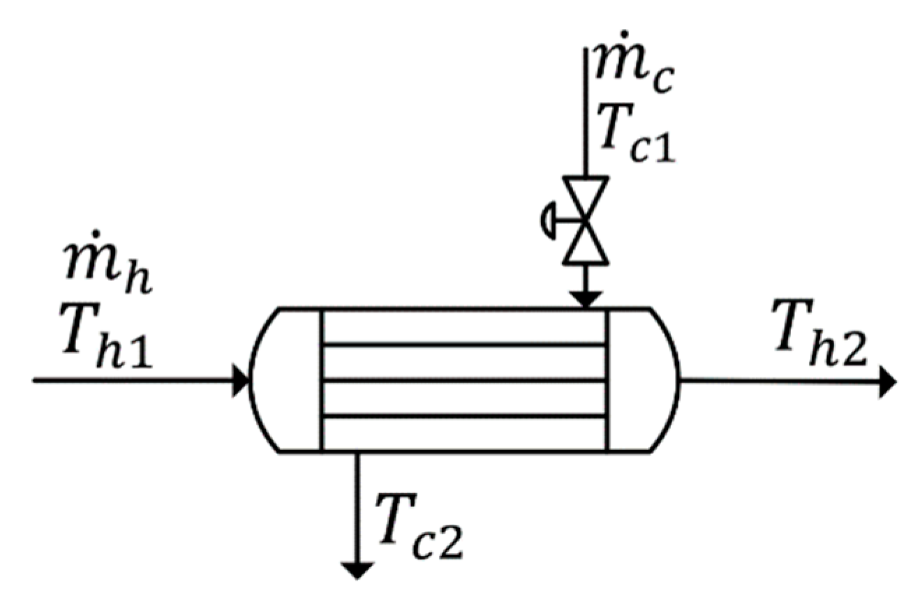
Figure 1 shows the sketch of a heat exchanger where a hot process fluid is cooled using a cold utility stream. We indicate with ${\dot{m}}_h$ and ${\dot{m}}_c$ the mass flows of the hot and cold fluids, respectively; with $T_{h1}$ and $T_{h2}$ the inlet and outlet temperatures of the hot fluid; and with $T_{c1}$ and $T_{c2}$ the inlet and outlet temperatures of the cold fluid. To simplify the discussion, we assume constant heat capacities ($c_{p,h}$ and $c_{p,c}$ for the hot and cold fluid, respectively), and perfect countercurrent flow in the heat exchanger.

The steady-state response of the heat exchanger to a change in the manipulated utility flow is strongly related to the exchanger design. Shinskey [1] showed that, by combination of the steady-state energy balance

$$\dot{q}={\dot{m}}_h{c}_{p,h}\left(T_{h1}-T_{h2}\right)={\dot{m}}_c{c}_{p,c}\left(T_{c2}-T_{c1}\right)$$

(1)

with the heat-exchanger design equation

$$\dot{q}=UA\frac{\left(T_{h1}-T_{c2}\right)-\left(T_{h2}-T_{c1}\right)}{\ln \left(\frac{T_{h1}-T_{c2}}{T_{h2}-T_{c1}}\right)}$$

(2)

the following relation can be obtained

$$\Delta T_N=\frac{1-R}{\frac{1}{E}-R}.$$

(3)

In the above equations, $\dot{q}$ is the rate at which heat is transferred between the two fluids in the heat exchanger, $U$ is the overall heat exchange coefficient (which is assumed invariant with respect to the flows), $A$ is the area available for heat exchange, $\Delta T_N$ is the normalized (dimensionless) hot fluid outlet temperature, defined as

$$\Delta T_N=\frac{T_{h2}-T_{c1}}{T_{h1}-T_{c1}},$$

(4)

and

$$R=\frac{{\dot{m}}_h{c}_{p,h}}{{\dot{m}}_c{c}_{p,c}},$$

(5)

$$E=\exp \left(\frac{UA}{{\dot{m}}_c{c}_{p,c}}-\frac{UA}{{\dot{m}}_h{c}_{p,h}}\right).$$

(6)

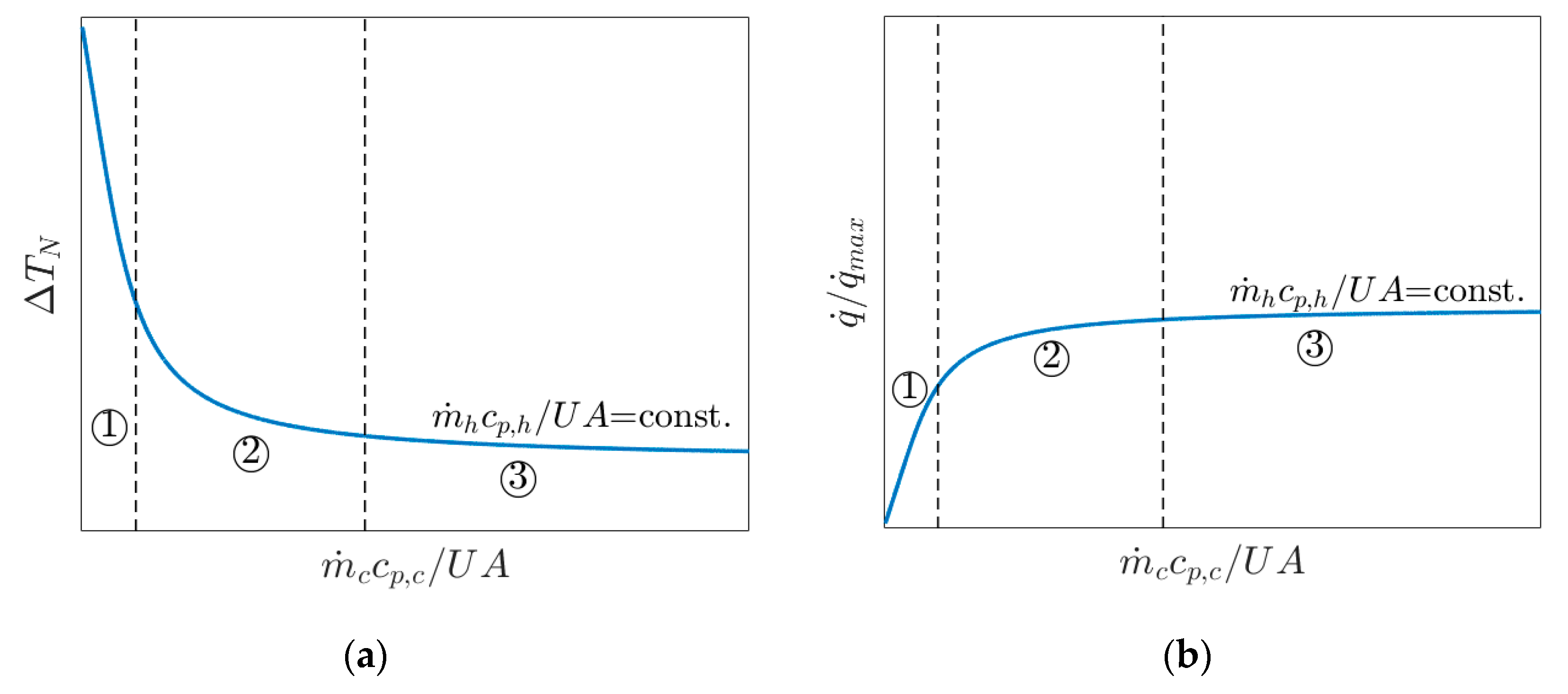
Equation (3) provides a dimensionless steady-state relation between the output to be controlled ($T_{h2})$ and the input to be manipulated (${\dot{m}}_c$) in the heat exchanger. This relation can be plotted as shown qualitatively in Figure 2a for an assigned value of ${\dot{m}}_h{c}_{p,h}/\left(UA\right)$, hence for an exchanger of assigned size.

In the heat-exchanger design task, we assume that the following variables are assigned: ${\dot{m}}_h$, $T_{h1}$, $T_{h2}$ and $T_{c1}$; hence, the nominal heat-exchanger duty $\dot{q}$ is set. This leaves the designer with the possibility of assigning one (and only one) of the following three variables: exchanger area, nominal utility flowrate, nominal utility outlet temperature. Setting one variable automatically determines the other two, and the resulting nominal operating condition of the heat exchanger can then be represented in the curve of Figure 2a. For example, for an assigned exchanger area (i.e., for a given curve in Figure 2a), a horizontal line through the nominal value of $\Delta T_N$ allows one to identify on the curve the nominal operation point of the heat exchanger, from which the required value of ${\dot{m}}_c$ is found. The nominal operation point may fall in one of the three regions highlighted in the figure: region ① is characterized by small utility flows (along with high utility outlet temperatures); region ③ is characterized by large utility flows (along with low utility outlet temperatures); region ② is in between. In several practical cases, the designer assigns $T_{c2}$ because a maximum allowed value may exist for it (e.g., maximum allowed temperature for cooling water, CW). This sets ${\dot{m}}_c$, and consequently the required area, as well as the exchanger nominal operation region.

The slope of the tangent to the curve in Figure 2a at each value of ${\dot{m}}_c$ represents the steady-state gain $K_P$ of the input-output pair ${\dot{m}}_c-T_{h2}$ [1,2]. Therefore, the resulting heat-exchanger operation region impacts on heat-transfer control. A heat exchanger designed within region ① results in a fairly constant value of $K_P$ at different values of ${\dot{m}}_c$, a desirable situation for control. A design in region ② is characterized by a steady-state gain that changes significantly with ${\dot{m}}_c$, which is not very favorable. Finally, if the heat exchanger is designed to operate within region ③, the steady-state gain is constant but very small, which can limit the achievable control performance.

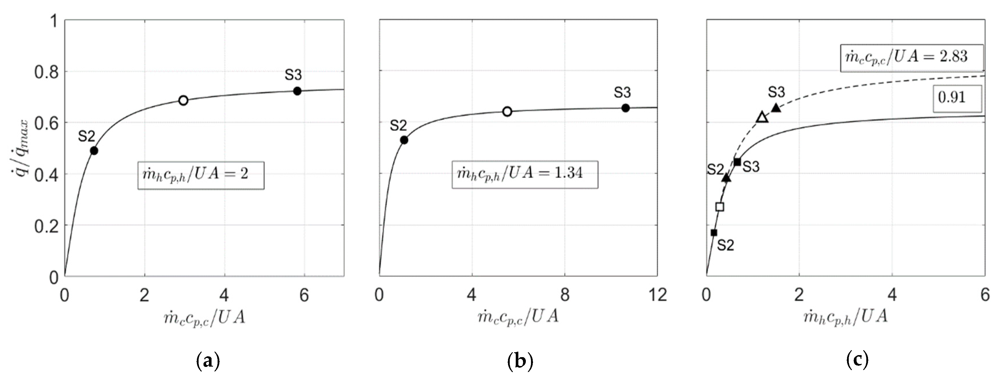
Shinskey [1] showed that also the exchanger duty can be made dimensionless and plotted against the dimensionless utility flow, resulting in

$$\frac{\dot{q}}{{\dot{q}}_{max}}=\frac{1-E}{\frac{UA}{{\dot{m}}_h{c}_{p,h}}-E\frac{UA}{{\dot{m}}_c{c}_{p,c}}}.$$

(7)

where ${\dot{q}}_{max}=UA\left(T_{h1}-T_{c1}\right)$. Equation (7) is illustrated qualitatively in Figure 2b, which highlights how the duty of a cooler of given area can be changed by adjusting the utility flow. A cooler designed in region ① (small utility flows) can effectively handle changes in the heat rate (e.g., resulting from increased capacity demand), therefore offering greater process rangeability; however, for a cooler designed in region ③ (large utility flows), the sensitivity of heat transfer to the utility flow is very low.

Note that also the dynamics of the input-output response is affected by the selected heat-exchanger design region. Larger exchangers (greater areas) typically result in slower responses, although the extent of the statement also depends on the selected exchanger layout.

2.2. Bypass Heat-Exchanger Configuration

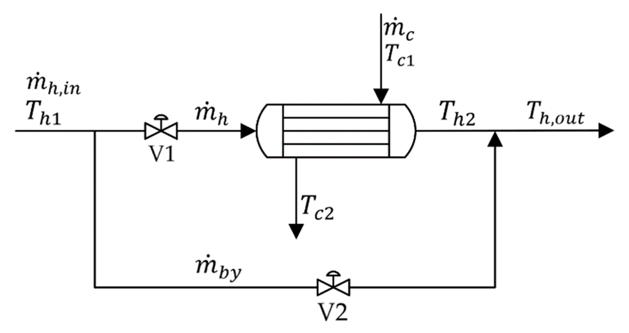
The use of a bypass stream is particularly useful when a utility stream is not available, e.g., when the cold fluid is a process stream whose flowrate cannot be adjusted due to upstream or downstream requirements. Figure 3 shows the most popular bypass configuration [8], where the bypassed stream is the same whose temperature is to be controlled. We denote the streams that enter and exit the heat exchanger with the same symbols as in the conventional configuration of Figure 1; instead, we indicate with ${\dot{m}}_{h,in}$ the mass flow of the hot fluid entering the overall system, with ${\dot{m}}_{by}$ the bypass stream mass flow, and with $T_{h,out}$ the hot fluid temperature after the mixing point (i.e., at the system exit). A typical heat-transfer control configuration aims at keeping $T_{h,out}$ at the desired value by manipulating valves V1 and V2 according to a complementary split-range arrangement [8,10] as summarized in

Table 1. Relation between controller output (CO) and valve opening in the complementary split-range temperature control arrangement. Notice that the two valves have opposite fail positions.

CO (%)	$\mathbf{V}1 \mathbf{Opening} \left(\mathit{\%}\right)$	$\mathbf{V}2 \mathbf{Opening} \left(\mathit{\%}\right)$
$0$	$100$	0
$50$	$50$	50
$100$	$0$	100

.

With respect to heat-exchanger design, the same considerations on $\Delta T_N$ and $\dot{q}/{\dot{q}}_{max}$ can be drawn as for the conventional configuration, and similar qualitative profiles as in Figure 2 can be observed. However, the flow appearing in the x axis (manipulated flow) is now ${\dot{m}}_h$ and not ${\dot{m}}_c$, and it can range between zero and ${\dot{m}}_{h,in}$. Assume that the same nominal heat rate $\dot{q}$ as in a conventional configuration is to be exchanged. Although the cold fluid outlet temperature $T_{c2}$ may be assigned by process requirements, in a heat exchanger with bypassing the designer can arbitrarily assign the flow ${\dot{m}}_h$ of hot fluid through the exchanger, to which the required $\dot{q}$ is to be transferred. For a given choice of ${\dot{m}}_h$ (or, equivalently, of ${\dot{m}}_{by}$, since ${\dot{m}}_{h,in}={\dot{m}}_h+{\dot{m}}_{by}$), there will be a different value of $T_{h2}$ that enables obtaining the desired temperature $T_{h,out}$ at the mixing point. The heat-exchanger area will be determined consequently. Therefore, the key design difference between a bypass heat exchanger and a conventional one is that, in a heat exchanger with bypassing, by assigning the design bypass flow the designer can set the exchanger nominal operation region, even if a constraint exists on the cold fluid outlet temperature; that cannot be done in a conventional exchanger. The price to pay is that, since $T_{h2}<T_{h,out}$, the mean temperature difference in the bypass exchanger is smaller than in a conventional one, and the resulting area is therefore greater.

Figure 2b can provide a graphical visualization of the impact of the flowrate through the heat exchanger on the steady-state response. As such, it offers a rationale for assigning the design bypass flowrate. As we will demonstrate later, a heat exchanger with bypassing becomes effective in terms of increased rangeability when the design bypass flow is assigned so that the exchanger operates within region ① at nominal conditions.

From the heat-exchanger dynamics point of view, one advantage of the bypass configuration is that adjustment of the temperature at the mixing point is much faster than at the exchanger exit [1,2,3], and this can improve temperature control. If we neglect transportation delays and sensor lags, the open-loop response of $T_{h,out}$ to a change in the temperature controller output p can be determined from a block-diagram representation of the system as illustrated in Figure 4, where variables indicated are defined in the Laplace domain.

We assume that the valves have first order dynamics (with steady-state gain $K_v$, time constant ${\tau }_v$, and transfer functions $G_{v1}\left(s\right)$ and $G_{v2}\left(s\right)=-G_{v1}\left(s\right)$, respectively), and that the heat exchanger has first-order dynamics with steady-state gain $K_{he}$, time constant ${\tau }_{he}$, and transfer function $G_{he}\left(s\right)$. Note that typically ${\tau }_v\ll {\tau }_{he}$. The three gains $K_1$, $K_2$ and $K_3$ shown in Figure 4 can be determined from steady-state considerations under the assumption that the mixing has no dynamics. It follows that (the prime symbol ′ denotes a deviation variable):

$$K_1=\frac{\partial T_{h,out}^{\prime }}{\partial \dot{m_h^{\prime }}}=\frac{T_{h2}}{{\dot{m}}_{h,in}},$$

(8)

$$K_2=\frac{\partial T_{h,out}^{\prime }}{\partial \dot{m_{by}^{\prime }}}=\frac{T_{h1}}{{\dot{m}}_{h,in}},$$

(9)

$$K_3=\frac{\partial T_{h,out}^{\prime }}{\partial T_{h2}^{\prime }}=\frac{{\dot{m}}_h}{{\dot{m}}_{h,in}},$$

(10)

where all variables in (8)–(10) are evaluated at steady state. By block diagram algebra, one can derive the open-loop transfer function:

$$G_p\left(s\right)=\frac{T_{h,out}^{\prime }\left(s\right)}{P^{\prime }\left(s\right)}=K_p\frac{{\tau }_{a}s+1}{\left({\tau }_{he}s+1\right)\left({\tau }_{v}s+1\right)},$$

(11)

whose parameters are:

$$K_p=K_v\left(K_2-K_1-K_3{K}_{he}\right)=K_V\frac{T_{h1}-T_{h2}-K_{he}{\dot{m}}_h}{{\dot{m}}_{h, in}},$$

(12)

$${\tau }_a=\frac{{\tau }_{he}\left(K_2-K_1\right)}{\left(K_2-K_1-K_3{K}_{he}\right)}=\frac{T_{h1}-T_{h2}}{T_{h1}-T_{h2}-K_{he}{\dot{m}}_h}.$$

(13)

Hence, the open-loop response of the heat exchanger with bypassing is second-order with numerator dynamics, and the lead time ${\tau }_a$ depends on the nominal hot flow through the heat exchanger (hence on the design bypass flow). If the valve dynamics can be neglected, the response is that of a lead-lag system. Note that since the exchanger size changes with ${\dot{m}}_h$, also the exchanger time constant ${\tau }_{he}$ depends on the bypass flow.

3. Process and Simulation

To quantitatively discuss the relation between heat-exchanger design and control in the light of the steady-state relations discussed above, we use a numerical example based on the same CHA manufacturing process described by Luyben [8]. The reaction studied is the hydrogenation of aniline to CHA:

$${\mathrm{C}}_6{\mathrm{H}}_5{\mathrm{NH}}_2+3{\mathrm{H}}_2\to {\mathrm{C}}_6{\mathrm{H}}_{13}\mathrm{N}.$$

(14)

The overall reaction rate $ℛ$ is given by:

$$ℛ=V_{R}k{C}_A{C}_H,$$

(15)

where $C_A$ and $C_H$ (${\mathrm{kmol}\mathrm{m}}^{-3})$ are the aniline and hydrogen concentrations in the liquid-phase respectively, $V_R$ is the reactor volume $\left({\mathrm{m}}^3\right)$, and $k$ (${\mathrm{m}}^3{\mathrm{kmol}}^{-1}{\mathrm{s}}^{-1}$) is the kinetic constant:

$$k=k_0{e}^{\frac{-\Delta E}{RT}}.$$

(16)

In the Arrhenius Equation (16), $k_0$ is the pre-exponential factor ($2\times {10}^4 {\mathrm{m}}^3{\mathrm{kmol}}^{-1}{\mathrm{s}}^{-1}$), ∆E the activation energy ($\mathrm{11,111}{\mathrm{kcal}\mathrm{kmol}}^{-1})$, $R$ the ideal gas constant $(1.987 {\mathrm{kcal}\mathrm{kmol}}^{-1}{\mathrm{K}}^{-1})$, and $T \left(\mathrm{K}\right)$ the reactor temperature.

The reaction is carried out in a continuously-stirred tank reactor and is exothermic. Hence, heat-transfer control is crucial for this process. As will be discussed later, three of the four flowsheets under investigation involve a jacketed reactor; in the fourth one, an external heat exchanger provides the required heat transfer to the reacting mass directly.

Under nominal operating conditions, the reactor is fed with $50 {\mathrm{kmol}\mathrm{h}}^{-1}$ of aniline and $200 {\mathrm{kmol}\mathrm{h}}^{-1}$ of hydrogen, and produces $47.6{\mathrm{kmol}\mathrm{h}}^{-1}$ of product at 99.7 mol% CHA concentration. The reactor temperature and pressure are 400 K and 20 atm, respectively, and the nominal heat rate to be removed is 2170 kW. While we keep the same reactor volume ($V_R=34 {\mathrm{m}}^3$) as in [8], we slightly adjust the reactor layout to obtain an aspect ratio and jacket width as recommended in [11]. This results in a reactor diameter of 2.6 m, a reactor height of 7.8 m (with a nominal level of 7.0 m), a jacket volume of $8 {\mathrm{m}}^3$, and a jacket exchange area of $70 {\mathrm{m}}^2$. The overall heat transfer coefficient through the jacket is set to $620 {\mathrm{W}\mathrm{m}}^{-2} {\mathrm{K}}^{-1}$ and it is assumed constant. All simulations have been carried out using Aspen Plus V11 and the dynamic counterpart Aspen Plus Dynamics V11.

4. Plant Design Alternatives

The process described in the previous section is developed according to four different flowsheets (plant designs), as illustrated in Figure 5. The designs differ for the way the heat of reaction is removed from the system. Namely, two designs (Figure 5b,d) remove the heat generated by the reaction using a two-surface arrangement: the reaction heat is first transferred from the reactor to a jacket, and then from the jacket to a heat exchanger. The other two designs exchange heat through one single surface: either a jacket (Figure 5a) or a heat exchanger (Figure 5c). Notice that whereas the jacket area depends on the reactor geometry and is therefore assigned, the heat-exchanger area is subject to design. As discussed in Section 2, different designs can determine different responses of the heat exchanger during operation, thus impacting on the reactor operation as well. The main characteristics of the plant designs are summarized in

Table 2. Summary of the main characteristics of the proposed plant designs.

	Design A	Design B	Design C	Design D1	Design D2
$\mathrm{Jacket}\mathrm{water}\mathrm{inlet}\mathrm{temperature}\left(\mathrm{K}\right)$	$332$	$332$	/	$332$	332
$\mathrm{Jacket}\mathrm{water}\mathrm{outlet}\mathrm{temperature}\left(\mathrm{K}\right)$	$349$	$349$	/	$349$	349
$\mathrm{Water}\mathrm{outlet}\mathrm{temperature}\mathrm{from}\mathrm{the}\mathrm{exchanger}\left(\mathrm{K}\right)$	/	$315$	315	$315$	315
$\mathrm{CHA}\mathrm{inlet}\mathrm{temperature}\mathrm{to}\mathrm{the}\mathrm{exchanger}\left(\mathrm{K}\right)$	/	/	$400$	/	/
$\mathrm{Exchanger}\mathrm{CHA}\mathrm{inlet}\mathrm{temperature}\left(\mathrm{K}\right)$	/	/	$356$	/	/
$\mathrm{Jacket}\mathrm{inlet}\mathrm{flowrate}\left({\mathrm{kg}\mathrm{s}}^{-1}\right)$	$30$	$30$	/	$30$	30
$\mathrm{Recycled}\mathrm{CHA}\mathrm{flow}\mathrm{to}\mathrm{reactor}\left({\mathrm{kmol}\mathrm{h}}^{-1}\right)$	/	/	$784$	/	/
$\mathrm{Bypassed}\mathrm{flowrate}\left({\mathrm{kmol}\mathrm{h}}^{-1}\right)$	/	/	/	3400	1000
$\mathrm{Cooling}\mathrm{water}\mathrm{flowrate}\left({\mathrm{kg}\mathrm{s}}^{-1}\right)$	$11.8$	$51$	$55$	51	51
Heat-exchanger duty (kW)	2170	2170	2315	2170	2170
Heat-exchanger area $\left({\mathrm{m}}^2\right)$	/	$48$	$47$	$142$	54
Heat-exchanger nominal operation region	/	③	③	①	②

.

4.1. Design A: Jacket Cooling with No Heat Exchanger

In this configuration (Design A; Figure 5a), we feed CW directly into the jacket to remove heat at the required rate. Given that the reactor temperature and the heat rate to be removed through the jacket are assigned, the jacket temperature remains assigned as well, and is equal to 349 K. This shows a strong limitation of this configuration, because such a high temperature is typically not admissible for CW. Nevertheless, it is instructive to consider this configuration as a term of comparison for assessing the overall heat-transfer control performance. Assuming that the CW is available at 305 K, a nominal CW flow of 11.8 kg/s is required. A high recirculation rate (30 kg/s) is maintained in the jacket to speed up the jacket dynamics and to linearize its response [1,12].

4.2. Design B: Jacket Cooling with External Cooler

Design B (Figure 5b) uses an external cooler to cool down the hot jacket water. This allows one to recirculate demineralized water in the jacket, which avoids the CW temperature concern discussed for design A. The jacket water has a nominal flow of 30 kg/s, enters the jacket at 332 K and exits at 349 K. The utility stream for the cooler is CW (305/315 K nominal inlet/outlet temperatures, 52 kg/s the required nominal flow). For a nominal $U=1503 {\mathrm{W}\mathrm{m}}^{-2}{\mathrm{K}}^{-1}$, the resulting heat-exchanger area is 48 m², and the exchanger design falls within region ③ (open circle in Figure 6a).

4.3. Design C: Direct Cooling with No Jacket

In the design shown in Figure 5c (Design C), the rationale is to remove the required heat rate by direct cooling of the reaction mass through an external cooler. Safety reasons may suggest this design: in fact, high circulation rates can provide very good mixing, which reduces the chance of hot-spot occurrence. Additionally, this system is useful when the cooling jacket area limits the achievable heat transfer [12]. One disadvantage is that the heat exchanger is required to cool down also the product stream, and therefore its nominal duty is increased. We consider a flow of 784 kmol/h of reacting mass through the cooler, of which 736.4 kmol/h are returned back to the reactor. For the same inlet and outlet CW temperatures (305/315 K), the required CW flow is 55 kg/s. With $U=807 {\mathrm{W}\mathrm{m}}^{-2} {\mathrm{K}}^{-1}$, the resulting heat exchanger area is 47 m², and the relevant design is in region ③ (open circle in Figure 6b).

4.4. Design D: Jacket Cooling with Bypass Heat Exchanger

The fourth design (Design D; Figure 5d) is the same one discussed in [8], and includes a heat exchanger with bypassing that cools down the hot water circulating in the jacket. The CW flow through the heat exchanger is not manipulated; therefore, this design may be considered also for heat integration. Net of the work done by the circulation pumps, the heat-exchanger duty is the same as that of design B (design C adds up also the duty related to product cooling); hence, for the same CW inlet and outlet temperatures, the required CW flow is also the same. However, now the nominal manipulated flow (hot stream through the heat exchanger, or equivalently bypass flow) can be set arbitrarily within the available flowrate range, and this allows the designer to assign the exchanger operation region under nominal operating conditions. To clarify this, within the same plant design, we consider two alternative designs for the heat exchanger. In Design D1, we set the design bypass flow to 3400 kmol/h (57% of the total hot fluid flow, i.e., very similar to the fraction of flow used in [8]), thus making the hot flow through the heat exchanger equal to 2600 kmol/h. With $U=1254 {\mathrm{W}\mathrm{m}}^{-2}{\mathrm{K}}^{-1}$, the resulting heat-exchanger area is 142 m², and the relevant design is in region ① (Figure 6c, open square). In Design D2, we use a smaller bypass flow (1000 kmol/h, or 17% of the total, hence close to the indications provided by existing rules of thumb [3,7]); this makes the hot flow through the heat exchanger equal to 5000 kmol/h, which results in a greater mean temperature difference, a slightly greater $U$ (1420 ${\mathrm{W}\mathrm{m}}^{-2}{\mathrm{K}}^{-1}$), and a considerably smaller exchanger (54 m²); the heat exchanger gets designed in operation region ② (Figure 6c, open triangle).

5. Control Performance Comparison

For each of the plant designs discussed in the previous section, we develop a different reactor temperature control scheme (Figure 7). Except for reactor temperature control, the basic control loops (feeds and inventory control) are the same in all schemes. Namely, the aniline feed is flow-controlled; the hydrogen feed is ratioed to the aniline feed; the reactor pressure is controlled by manipulating the gaseous flow leaving the reactor; the reactor level is controlled by adjusting the liquid product flow. In Design D, the recirculation flow through the jacket is kept constant using a variable speed pump, as recommended in [8]. The jacket level control loop in Figure 7a is not indicated to avoid cluttering the drawing.

In all schemes, the reactor temperature is controlled via a cascade system, where the output signal from the master reactor temperature controller (TC-101) becomes the remote setpoint (RSP) for the slave temperature controller (TC-102) that manipulates either the CW flow (valve V7 in plant Designs A, B and C), or the bypass and hot fluid flows (valves V2 and V1 in plant design D). The cooling water valve V7 is fail-open in all schemes; valves V2 and V1 are arranged as indicated in Table 1. The valve position controller (VPC-101) is switched on only during control Scenario 3.

The performance of each control scheme is assessed under three scenarios:

• Scenario 1: rejection of a disturbance in the aniline feed temperature; at $t=1$ h, the aniline temperature ramps up by 20 K in 1 h;
• Scenario 2: rejection of a disturbance in the aniline feed flow; at $t=1$ h, the aniline flow is step-decreased by 20%;
• Scenario 3: productivity increase; starting from $t=1$ h, the aniline feed is increased until the maximum plant capacity is reached.

With respect to Scenario 3, when productivity increases, more heat is released in (and must be removed from) the reactor. Therefore, plant productivity is limited by the available plant cooling capacity. In all control schemes, the increase in productivity is managed by VPC-101, which increases the setpoint to the aniline flow controller until the valve that sets the plant cooling capacity becomes almost fully open. In plant designs A, B and C, this situation corresponds to the CW valve V7 reaching (say) 90% opening, whereas in plant design D it corresponds to V1 reaching 90% opening (or, equivalently, V2 reaching 10% opening).

We did not attempt to optimize the tuning of the proportional-integral temperature controllers. Rather, we coarsely tuned them using the relay autotuning method [13], with subsequent field adjustment to improve the closed-loop response if required. The integral-only VPC controllers were tuned in such a way as to provide a very smooth transition to the plant maximum capacity.

The control performances for the three control scenarios are illustrated in Figure 8 (Design A), Figure 9 (Design B), Figure 10 (Design C), Figure 11 (Design D1) and Figure 12 (Design D2).

5.1. Control Scenario 1

The feed temperature disturbance is compensated for very effectively in all plant designs. This is because the required increase in the heat duty is relatively small, and can be handled well by an increase of the CW flow (Designs A, B and C), or by a decrease of the bypass flow (Designs D1 and D2), with no valve saturation in either case. Yet, Design B and Design C (both with a heat exchanger nominally operating in region ①) require a stronger increase of the CW flow. Design D2 (exchanger in region ②) also suffers a bit, because the disturbance makes the bypass flow decrease to almost zero.

5.2. Control Scenario 2

Notwithstanding the severity of the disturbance, Designs A, D1 and D2 are able to reject it very quickly: it takes about 0.5 h to bring the reactor temperature back to its setpoint, with a modest undershoot (~1 K). This is achieved by an aggressive action on the CW flow in design A; probably, a less aggressive tuning of TC-101 in this design might work better, but this is unimportant for this discussion.

Also Designs B and C do a good job in rejecting the disturbance, even if the settling time and the reactor temperature undershoot are slightly greater (~1 h and ~2 K) than for the other designs. Notice that, at the new steady state, the output signal from TC-102 is about 90% in both designs, meaning that the CW valve is almost fully closed. This does not occur for either Design A or Designs D1 and D2.

5.3. Control Scenario 3

Upon a request to maximize the productivity, VPC-101 makes the aniline flow controller slowly admit more feed to the reactor, until valve V7 becomes 90% open (Designs A, B and C), or valve V2 10% open (Designs D1 and D2). In all cases, the reactor temperature is controlled perfectly. However, the resulting steady-state increase in the feed (with respect to the nominal one) is strongly different: 26% in Design A, less than 4% in Designs B and C, 21% in Design D1, and 3% in Design D2 (note that, for ease of discussion, in Scenario D2 we reduce from 10% to 1% the setpoint of VPC-101).

6. Discussion

Were it not for the limitation on the maximum allowed jacket fluid temperature, Design A would be the one preferred for the process under investigation: it is simple, has the smallest cost (no heat exchanger required), and guarantees excellent control performances in all tested scenarios.

The increased speed of response of heat exchangers with a bypass flow is not fully exploited in Design D, because the dynamics that is made faster is the one within the slave loop: while making the slave loop faster improves the performance of a cascade controller, the impact of this improvement is relatively small for this process, also due to the fact that in all designs high recirculation rates are maintained in the jacket. Therefore, the improved heat-transfer performance of Design D for this process is mainly due its steady-state characteristics. Dynamic controllability is much less of an issue for the problem under investigation.

Designs B and C are able to reject the severe disturbance of Scenario 2 effectively. To achieve this, the heat-exchanger duty must be significantly reduced. Given that under nominal conditions the heat exchangers operate in region ③ (small process gain), this strong steady-state decrease in the duty requires a strong change in the manipulated CW flow. This is illustrated in Figure 6a (for Design B) and Figure 6b (for Design C), where we use a closed circle with S2 heading to denote the new steady-state condition reached after the disturbance has been compensated for. It can be seen that, in order to restore the desired reactor temperature, we must travel far left on the duty curve: this is the reason why the TC-102 output signal almost hits its upper limit in both designs. Note (Figure 10b) that this strong decrease in the CW flow has also a negative impact on the CW outlet temperature. Design D1 is facilitated in handling this disturbance, because the heat exchanger is designed to operate nominally in the high-gain region ①, where a small change in the manipulated flow significantly impacts on the duty; the required travel on the duty curve (Figure 6c, closed square with S2 heading on the full line) is therefore small. More effort is required in design D2 (Figure 6c, closed triangle with S2 heading on the broken line), due to the exchanger design in region ②.

When it comes to a productivity increase (Scenario 3), we must travel right on the duty curves of Figure 6 in order to increase $\dot{q}$. However, while travelling to the left can always result in a significant heat rate decrease (net of valve rangeability issues, we can always significantly reduce a flow by closing a valve), moving to the right is much less effective if the travel is to be done within a low-gain region. For example, the travel is effective for design D1 (Figure 6c, closed S3 square): a small increase in ${\dot{m}}_h$ suffices to significantly increase $\dot{q}$, hence to allow for a significant increase of the reactor feed. Designs B and C suffer from the fact that even a large change in the CW flow can cause only a small change in the exchanger duty (Figure 6a,b, closed S3 circles); therefore, the increase in productivity can be very limited in these designs. Notice that also Design D2 (which operates within region ② at nominal conditions) suffers from the same problem.

A graphical representation like the one in Figure 6c clearly illustrates why and when a heat-exchanger with bypassing can be more effective than a standard one in handling capacity changes. Namely, the bypass configuration works well if the design bypass flowrate is sufficiently large as to make the heat exchanger operate within region ① at nominal conditions. For the process under investigation, this occurs for a rather large bypass fraction (57%, Design D1), whereas a smaller fraction (17%; Design D2) is insufficient (although it would look meaningful according to existing good engineering practice guidelines [3,7]). This representation can therefore help the designer in assigning the design fraction of flow to be bypassed in a heat exchanger, avoiding the need for extended simulations.

7. Conclusions

The effectiveness of heat-exchanger bypass control in heat transfer operations can be significant even if the favorable dynamics of the bypass configuration is not exploited in full. The advantages are related to how the bypass heat exchanger responds at steady state to changes in the manipulated flow. Using heat-exchanger design arguments, we have shown graphically why a bypass heat exchanger can provide wider rangeability in processes where heat transfer is required. The reason is that, by using a bypass stream, the designer can assign the heat-exchanger operation region. Namely, the heat exchanger can be designed to operate in a region where the steady-state gain of the temperature/flow pair is relatively high (and constant). Consequently, the heat-exchanger duty can be modulated over a wide range of values to accommodate even large changes in the process capacity.

We showed that, on the other hand, under the same design constraints existing for a heat exchanger with bypassing, the operation region of a heat exchanger with no bypassing cannot be assigned by the designer, because it becomes a result of the design exercise. Therefore, if the process requirements make the heat exchanger be designed in a region where the steady state gain is very small, the heat-exchanger (hence, the process) rangeability is severely limited.

Since the operation region of a bypass heat exchanger depends on the design bypass flowrate, visualizing graphically the region within which the heat exchanger operates can be useful to assign the design fraction of flow to be bypassed. This can provide a theoretical foundation for existing rules of thumb for bypass flowrate selection, and it can help the designer to quickly assess whether a given bypass design can be effective or not, with no need to resort to extensive simulations.

References

1. Shinskey, G.F. Process Control Systems, Application, Design and Tuning; McGraw-Hill: New York, NY, USA, 1988. [Google Scholar]
2. McMillan, G.K.; Taormina, C.M. Advanced Temperature Measurement and Control; Instrument Society for Measurement and Control: Research Triangle Park, NC, USA, 1995; pp. 95–100. [Google Scholar]
3. Luyben, W.L.; Tyréus, B.D.; Luyben, M.L. Plantwide Process Control; McGraw-Hill: New York, NY, USA, 1999. [Google Scholar]
4. Bequette, W.B. Process Control: Modeling, Design and Simulation; Prentice-Hall: Upper Saddle River, NJ, USA, 2003. [Google Scholar]
5. Riggs, J.B.; Karim, N.M. Chemical and Bioprocess Control; Ferret Publishing: Austin, TX, USA, 2007. [Google Scholar]
6. Diaz-Bejarano, E.; Pelloja, G.; Coletti, F.; Macchietto, S. Heat exchanger bypass control to mitigate the cost of fouling in refinery preheat trains. Chem. Eng. Trans. 2015, 43, 2119–2124. [Google Scholar]
7. Jones, W.E.; Wilson, J.A. An introduction to process flexibility. Part 1. Heat exchange. Chem. Eng. Educ. 1997, 31, 172–177. [Google Scholar]
8. Luyben, W.L. L. Heat-exchanger bypass control. Ind. Eng. Chem. Res. 2011, 50, 965–973. [Google Scholar] [CrossRef]
9. Manenti, G. A calculation procedure for a heat exchanger and bypass equipment. Comput. Chem. Eng. 2011, 35, 2378–2388. [Google Scholar] [CrossRef]
10. Kuphaldt, T.R. Basic Principles of Control Valves and Actuators. In Lessons in Industrial Instrumentation; 2018; Available online: https://control.com/ (accessed on 4 January 2021).
11. McKetta, J.J. Heat Transfer Design Methods; Marcel Dekker: New York, NY, USA, 1992. [Google Scholar]
12. Luyben, W.L. Chemical Reactor Design and Control; Wiley: Hoboken, NJ, USA, 2007. [Google Scholar]
13. Seborg, D.E.; Edgar, T.F.; Mellichamp, D.A.; Doyle, F.J. Process Dynamics and Control, 4th ed.; Wiley: Hoboken, NJ, USA, 2017. [Google Scholar]
Figure 1. Simplified scheme of a cooler, where manipulation of the cold utility flow is allowed.
Processes 09 00244 g001
Figure 2. Steady-state profile of the dimensionless (a) hot fluid outlet temperature and (b) exchanger duty with respect to the dimensionless manipulated flow for a cooler with conventional configuration. The vertical dashed lines delimit the exchanger operation regions.
Processes 09 00244 g002
Figure 3. Simplified scheme of a bypass cooler, where manipulation of the hot bypass stream is allowed (the hot stream through the exchanger is adjusted accordingly in a complementary split-range arrangement).
Processes 09 00244 g003
Figure 4. Block-diagram representation of the bypass configuration for the heat exchanger.
Processes 09 00244 g004
Figure 5. Schemes of the four plant designs. (a) Design A: jacket cooling with no heat exchanger; (b) design B: jacket cooling with external cooler; (c) design C: direct cooling with no jacket; (d) design D: jacket cooling with bypass heat exchanger.
Processes 09 00244 g005
Figure 6. Operation regions for the heat exchangers in (a) Design B, (b) Design C, (c) Designs D1 (solid line) and D2 (broken line). The open symbols refer to the nominal operating conditions; the closed ones to the new steady-state conditions reached in control Scenario 2 (S2) and control Scenario 3 (S3). Note that both curves in (c) retain a physical meaning only up to a value of m ˙ h equal to the total flowrate of hot fluid.
Processes 09 00244 g006
Figure 7. Control scheme for (a) design A, (b) design B, (c) design C, (d) design D.
Processes 09 00244 g007
Figure 8. Control performance of plant Design A under (a) Scenario 1, (b) Scenario 2, and (c) Scenario 3.
Processes 09 00244 g008
Figure 9. Control performance of plant Design B under (a) Scenario 1, (b) Scenario 2, and (c) Scenario 3.
Processes 09 00244 g009
Figure 10. Control performance of plant Design C under (a) Scenario 1, (b) Scenario 2, and (c) Scenario 3.
Processes 09 00244 g010
Figure 11. Control performance of plant Design D1 under (a) Scenario 1, (b) Scenario 2, and (c) Scenario 3.
Processes 09 00244 g011
Figure 12. Control performance of plant Design D2 under (a) Scenario 1, (b) Scenario 2, and (c) Scenario 3.
Processes 09 00244 g012