Numerical Simulation of Dyeing Process of Cotton with Natural Dye

Abstract

Cotton dyeing is a very complex process with many variables in which different phenomena occur simultaneously. This study aimed to describe the cotton dyeing process by natural dye, using a mathematical model that consists of three mass conservation equations that depict dyeing cotton in cones, taking a representative volume element at the micro, meso, and macroscales. The first equation describes the concentration changes of the dye in the solution, taking into account the diffusive, convective, adsorptive, and reactive effects. The second equation describes the changes in dye concentration in cotton fiber, considering the diffusive, adsorptive, and reactive effects within an intermediate scale. The last equation describes changes in the concentration of dye in the solution on the macroscale, based on the characteristics of the equipment and the difference in concentration before and after passing through the fiber. In addition, a fluid continuity equation was incorporated, taking into account Darcy’s law. In the simulation of the dyeing process with synthetic dye with initial concentrations of 0.408 and 2.06 kg/m³, RMSE of 0.00221 and 0.0289 kg/m³ were obtained, respectively. For the simulation of a dyeing process with natural dyeing, a behavior similar to the experimental data was obtained.

1. Introduction

The use of non-allergic, non-toxic, and eco-friendly natural dyes in textiles has become a topic of great importance due to environmental awareness to avoid some dangerous synthetic dyes [1]. However, around the world, the use of natural dyes for textile coloring has been mainly limited to artisans and small-scale exporters and producers engaged in the production and sale of high-value eco-friendly textiles [2].

Recently, several commercial dyers and small textile exporting companies have begun to explore the possibilities of using natural dyes to dye and print textiles regularly to overcome the environmental pollution caused by synthetic dyes. Natural dyes produce very rare calming and soft shades compared to synthetic dyes [2].

On the other hand, dyeing is a very complex process, with many variables in which different phenomena co-occur [3]. The process requires a good understanding of different domains of science, including chemistry, physical chemistry, fluid mechanics, and thermodynamics. Designing the most efficient dyeing process generally involves concerns about machinery design, preselection of dyes with compatible properties, use of appropriate control profiles, e.g., pH versus time profiles, selection of liquor ratio, speed flow rates and reversal times of flow direction, and the type of temperature versus time profiles [4].

Mathematical modeling is a fundamental activity in different areas of science and engineering [5]. The formulation of qualitative and quantitative expressions about the phenomena observed and involved in a mathematical problem is the motivation for a total contribution to the development of these applications and advances in science and engineering [6,7,8]. The simulation of the process leads to a better understanding of this process. Furthermore, the simulation can be used in different scenarios (different dyes), with which the behavior of its kinetics can be predicted in order to be able to apply this information obtained to artisan dyeing processes.

The study leads to knowledge of the kinetics of dyeing, the behavior of the concentration of the dye within the dyeing vat, the fiber, and the solution in the porous media. In addition, it explains the different absorption and reaction phenomena that occur simultaneously. To establish dyeing time schedules, optimize energy use, and, perhaps most importantly, dismiss the environmental impact of the process [9,10], it requires the use of an established model to compare using natural dyes and adapt it to the operating conditions of artisans. This study only intends to cover the first part. The practical advantages of obtaining the numerical simulation are the following: (1) It improves the understanding of the different phenomena involved in the dyeing process. (2) To obtain a mathematical model able to predict the experimental data in order to modify the experimental conditions commonly used by artisans. This study was born from the need of some Oaxaca artisans (México) dedicated to dyeing typical clothes of the region and cotton handicrafts. Therefore, Curcuma Longa and other natural colorants are widely used, in addition to their easy acquisition. In these processes, the mordant is used as pretreatment.

The analysis developed by Guelli [11] makes it possible to improve the information at a microscale, composed of the textile fibers of the yarn in contact with the dyeing bath fluid, and at a macroscale, consisting of the cones of yarns inside the package.

The final mathematical model comprises three equations. The first describes the dye concentration in the dyeing bath liquid outside the cone (macroscale) [12,13]. The second predicts the dye concentration in the bath fluid surrounding the yarn but inside the cone, and the last equation evaluates the dye concentration in the fiber. Therefore, the model can calculate the various mass transfer resistances during the dyeing process. The final equation for the macroscale incorporates essential information from the intermediate and microscales, which allows the most accurate prediction of textile dyeing kinetics.

To solve the set of partial differential equations of the mathematical model, the authors developed a calculation code using the finite volume method [14]. This code used a generalized coordinate system to facilitate the application of boundary conditions to different cone geometries. The simulation demonstrates that the inclusion of the dispersion term in the dyeing model improves the simulation dyeing process results in dye absorption [15].

The objective of this work is to simulate the dyeing process using a model developed by Guelli et al. [11] and to obtain its numerical approximation of the set of equations using COMSOL Multiphysics 4.3b., in addition to simulating the same process with curcumin, a natural dye.

2. Simulation of Cotton Cone Dyeing

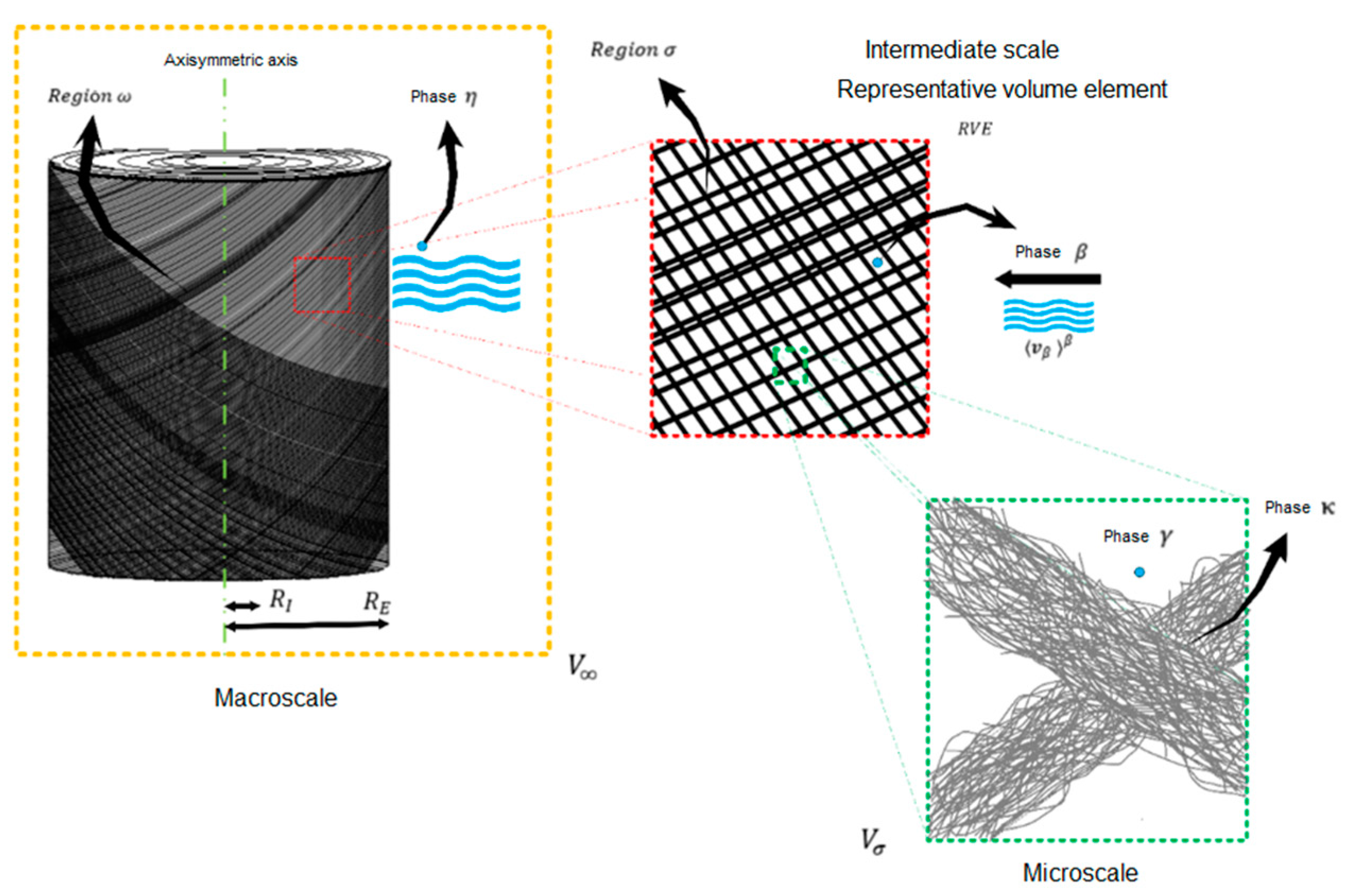
In this work, the model by Guelli et al. [11] was used, in which the cotton yarn cone system is divided into three scales, macro, meso, and micro, with their respective phases and regions, as shown in Figure 1. The representative volume of the macroscale (V_∞) is composed of the thread cone (region ω) and the dye solution (phase η) is its surroundings. The representative volume element of the mesoscale contains cotton fiber (region σ) and the dye solution (phase β), taking into account the average velocity of the fluid. The representative volume at the microscale is composed of microfibrils (phase κ) and dye solution (phase γ) [16].

2.1. System Geometry

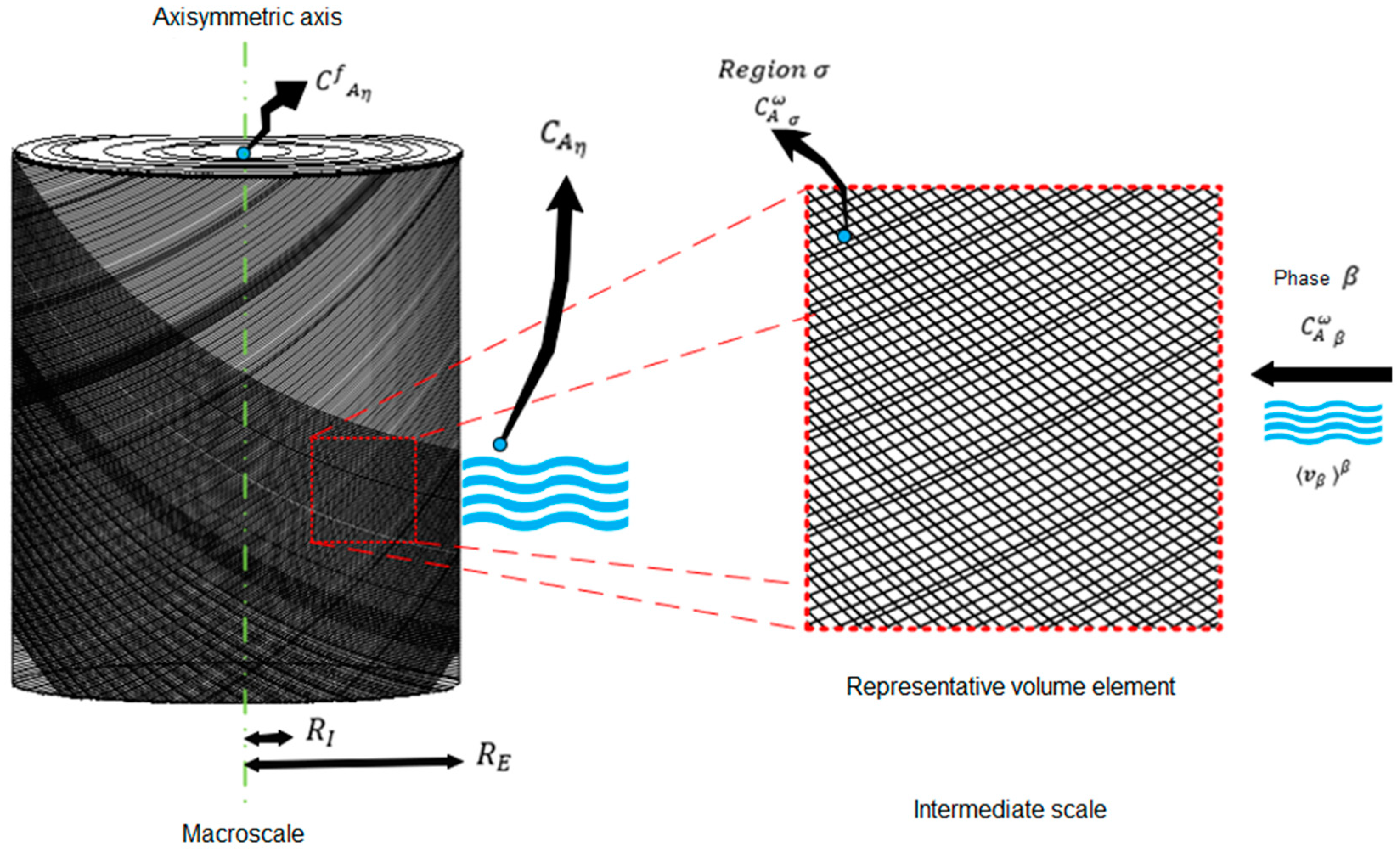
In the yarn cone dyeing processes, the cones can be cylindrical or conical. Therefore, the geometry is generalized to cylindrical cones. Due to the symmetry of the cone, the system’s geometry can be simplified by analyzing a half part of the 2D model, shown in Figure 2 (right part in the red square), using an axisymmetric axis. The figure shows the thread cone between the RE and RI boundaries. Moreover, this figure shows the direction of the flow exerted by the pump (black arrows).

2.2. Mass Conservation Equation in the Dyeing Process

2.2.1. The Macroscale

Three equations describe the dyeing process at the macroscale and the intermediate scale. The conservation equation for the macroscale (1) describes the change in concentration in the solution in the dyeing tank, which is dependent on the volumetric flow and is inversely proportional to the volume of the tank and reaches a final established concentration. Because perfect mixing is assumed, there will be no spatial variations, so an ordinary differential equation describes this process. Equation (2) describes the initial concentration condition of the solution.

$$\frac{d{C}_{A_{\eta }}}{dt}=\frac{Q}{V}\left(C_{A_{\eta }}-C^f{}_{A_{\eta }}\right)$$

(1)

$$C.I. C_{A_{\eta }}=C_{i } t=0$$

(2)

2.2.2. Mass Conservation Equations at the Mesoscale

The intermediate scale or mesoscale is described by two partial differential equations. The following equations describe the dye balance in the solution (Equation (3)) and in the fiber (Equation (7)). The second term describes the convective and diffusive transport mechanisms for solution and thread, respectively. The penultimate term of the equation represents the adsorption/desorption process, and the last term is the reactive term. Equations (4) and (8) are initial conditions for the solution and fiber, respectively, and Equations (5), (6), (9) and (10) are the boundary conditions shown in Figure 3.

Equation of conservation of mass of the liquid phase in the mesoscale

$${\epsilon }_{\beta }\frac{\partial C_A^{\omega }{}_{\beta }}{\partial t}+\nabla ·\left({\epsilon }_{\beta }{\langle {\mathit{v}}_{\beta }\rangle }^{\beta }{C}_A^{\omega }{}_{\beta }\right)=\nabla ·\left({\epsilon }_{\beta }{D}_{\beta }^{*}\nabla C_A^{\omega }{}_{\beta }\right)-a_v{|}_{\beta \sigma }h\left(C_A^{\omega }{}_{\beta }-C_A^{\omega }{}_{\sigma }\right)-\psi k_h{\epsilon }_{\beta }{C}_A^{\omega }{}_{\beta }$$

(3)

$$C.I. C_{A_{\beta }}=C_{i } t=0$$

(4)

$$C.F. 1 C_A^{\omega }{}_{\beta }=C_{A_{\eta }} ; interphase A_{\eta \omega }, on R_E$$

(5)

$$C.F.2 \nabla C_A^{\omega }{}_{\beta }=0 ; Interphase A_{\eta \omega }, on R_I$$

(6)

Equation of conservation of mass of the fiber region in the mesoscale

$${\epsilon }_{\sigma }{\epsilon }_{\gamma }\frac{\partial C_A^{\omega }{}_{\sigma }}{\partial t}=\nabla ·\left({\epsilon }_{\sigma }{D}_{\sigma }^{*}\nabla C_A^{\omega }{}_{\sigma }\right)+a_v{|}_{\beta \sigma }h\left(C_A^{\omega }{}_{\beta }-C_A^{\omega }{}_{\sigma }\right)+\psi \left(a_v{|}_{\gamma \kappa }k-k_h{\epsilon }_{\gamma }\right){\epsilon }_{\sigma }{C}_A^{\omega }{}_{\beta }+\Omega a_v{|}_{\gamma \kappa }{K}_{eq}{\epsilon }_{\sigma }\frac{\partial }{\partial t}{C}_A^{\omega }{}_{\sigma }$$

(7)

$$C.I. C_{A_{\sigma }}=C_{i } t=0$$

(8)

$$C.F. 1 C_A^{\omega }{}_{\sigma }=C_{A_{\eta }} ; Interphase A_{\eta \omega }, on R_E$$

(9)

$$C.F.2 \nabla C_A^{\omega }{}_{\sigma }=0 ; Interphase A_{\eta \omega }, on R_I$$

(10)

2.2.3. Continuity Equation in the Fluid Considering Darcy’s Law

In order to obtain the velocity field distribution, the continuity equation considers a porous medium.

$${\epsilon }_{\sigma }\frac{\partial {\rho }_s}{\partial t}+\nabla ·\left({\rho }_s{\langle {\mathit{v}}_{\beta }\rangle }^{\beta }\right)=0$$

(11)

$$C.I. P=P_{i } t=0$$

(12)

$$C.F. 1 P=P_0 ; on R_E$$

(13)

$$C.F.2 P=P_1; on R_I$$

(14)

It was considered a flow equation derived from Darcy’s law neglecting the effect of gravity [17].

$${\langle {\mathit{v}}_{\beta }\rangle }^{\beta }=-\frac{K_{\sigma }}{{\mu }_s}\nabla \langle p\rangle$$

(15)

Figure 3 shows the main variables that solve the mass conservation equations on the two scales. These equations are considered in the geometric structure used for the modeling and simulation of the process. $C_{A_{\eta }}$ is obtained from Equation (1) and the initial condition described in Equation (5), $C^f{}_{A_{\eta }}$ is obtained from $C_A^{\omega }{}_{\beta } en R_I.$ On the mesoscale, $C_A^{\omega }{}_{\beta }$ is obtained from Equation (3), $C_A^{\omega }{}_{\sigma }$ from Equation (7), and from Equations (11)–(15), the average velocity of the fluid is obtained.

2.3. State Equations

Table 1. Parameters used in the simulation [11].

Symbol	Value	Description
Geometric parameters
$d_1$	$0.041\left[\mathrm{m}\right]$	Cone inner diameter
$d_2$	$0.137\left[\mathrm{m}\right]$	Cone outer diameter
$H$	$0.128\left[\mathrm{m}\right]$	Cone height
Operational parameters
$RS$	$1/10$	Liquor ratio
$NC$	$16/2$	Number of cotton thread
$C_i$	$0.408\left[\frac{\mathrm{kg}}{{\mathrm{m}}^3}\right]$	Initial concentration of phase η
$C^f{}_{A_{\eta }}$	$0.0054688\left[\frac{\mathrm{kg}}{{\mathrm{m}}^3}\right]$	Concentration of the η phase after passing through the yarn fibers
${\rho }_f$	$1538.4615\left[\frac{\mathrm{kg}}{{\mathrm{m}}^3}\right]$	Cotton fiber density
${\rho }_{s60}$	$983.2\left[\frac{\mathrm{kg}}{{\mathrm{m}}^3}\right]$	Density of dye solution at 60 °C
${\mu }_{60}$	$0.0005\left[\frac{\mathrm{kg}}{{\mathrm{m}}^3}\right]$	Solution viscosity 60 °C
$P_0$	$\mathrm{101,330}\left[\mathrm{Pa}\right]$	Pressure at boundary 1, before the solution, passes through the porous medium
$P_1$	$\mathrm{101,325}\left[\mathrm{Pa}\right]$	Pressure at boundary 2, after the solution, passes through the porous medium
$K_{\sigma }$	$9.384\times {10}^{-10}\left[{\mathrm{m}}^2\right]$	Fiber region permeability
$Q$	$0.0009\left[\frac{{\mathrm{m}}^3}{\min }\right]$	Pump discharge flow
$V$	$0.007\left[{\mathrm{m}}^3\right]$	Dyeing container volume
${\epsilon }_{\gamma }$	$0.772$	Porosity in the microscale liquid phase
${\epsilon }_{\kappa }$	$0.228$	Porosity in the microscale fiber region
${\epsilon }_{\beta }$	$0.259$	Porosity in the liquid phase on the mesoscale
${\epsilon }_{\sigma }$	$0.771$	Porosity in the fiber region on the mesoscale
$D_{\beta xx}$	$1.008\times {10}^{-4}\left[\frac{{\mathrm{m}}^2}{\mathrm{s}}\right]$	Radial dispersion tensor in the liquid phase
$D_{\beta zz}$	$1.063\times {10}^{-5}\left[\frac{{\mathrm{m}}^2}{\mathrm{s}}\right]$	Axial dispersion tensor in the liquid phase
$D_{\sigma }^{*}$	$1.105\times {10}^{-10}\left[\frac{{\mathrm{m}}^2}{\mathrm{s}}\right]$	Effective diffusivity tensor in the fiber region
$a_v{|}_{\beta \sigma }$	$9920.7\left[\frac{1}{\mathrm{m}}\right]$	Interfacial area per unit volume on the intermediate scale
$h$	$1.67\times {10}^{-6.8}\left[\frac{\mathrm{m}}{\mathrm{s}}\right]$	Convective mass transfer coefficient
Kinetic and thermodynamic parameters
$k_{h1}$	$3.429\times {10}^{-4}\left[\frac{1}{\mathrm{s}}\right]$	Pseudo-first-order hydrolysis constant (before the addition of soda)
$k_{h2}$	$4.205\times {10}^{-3}\left[\frac{1}{\mathrm{s}}\right]$	Pseudo-first-order hydrolysis constant (after addition of soda)
$a_v{|}_{\gamma \kappa }{k}_1$	$4.933\times {10}^{-3}\left[\frac{1}{\mathrm{s}}\right]$	Reaction constant (before the addition of soda)
$a_v{|}_{\gamma \kappa }{k}_2$	$6.116\times {10}^{-3}\left[\frac{1}{\mathrm{s}}\right]$	Reaction constant (after the addition of soda)
$K_{eq}$	-	Constant equilibrium adsorption
Dyeing type definition parameters
$\psi$	1	Reactive dye variable
$\Omega$	0	Adsorptive dye variable

shows the parameters that describe the properties and conditions of the dyeing process used in the experimental tests of Guelli et al. [11], and these are used in the simulation of the process. The dyeing equipment used to obtain the experimental data was a pilot, and its capacity was a single cone [3]. For this purpose, we have the geometric parameters of the cone, the operational parameters of the dyeing equipment, and the properties that determine the phases and their interaction when in contact (dyeing solution and cotton fibers). Additionally, we have thermodynamic and kinetic parameters that describe the adsorption and chemical reaction phenomena [18] and, finally, the parameters that indicate the mechanism of dyeing, for example, adsorption and/or chemical reaction occur [19].

3. Numerical Solution

3.1. Computational Methodology Used to Solve the Equations of the Model

The equations and geometry described in Section 2 were implemented in COMSOL Multiphysics 4.3b, using the general and coefficient form PDE. The geometry was established in 2D axisymmetric form, as shown in Figure 2.

The initial value for the concentration in the solution on the mesoscale $\left(C_A^{\omega }{}_{\beta }\right)$ was considered equal to the initial concentration of the solution on the macroscale $\left(C_i\right)$. Therefore, the initial value of the concentration in the fiber on the mesoscale $\left(C_A^{\omega }{}_{\sigma }\right)$ was considered equal to zero. Thus, for the solution of the momentum conservation equation, the boundary conditions for the pressures P_0 and P_1 were 101,330 and 101,325 Pa, respectively.

The new values of $C_A^{\omega }{}_{\beta }$, $C_A^{\omega }{}_{\sigma }$ and the average velocity value ${\langle {\mathit{v}}_{\beta }\rangle }^{\beta }$, were calculated by solving Equations (3)–(14). The Darcy equation describes the transport of dye in porous media [20]. Then, to obtain the new value of the concentration of the solution on the macroscale, $C_{A_{\eta }}$ Equations (1) and (2) were solved.

The set of PDE (Equations (3), (7) and (11)) and the ODE (Equation (1)) were solved using COMSOL Multiphysics 4.3b, using the finite element method, with which were solved the primary variables in the space of the geometry and up to 2700 s. Using a transient study and the Multifrontal Massively Parallel sparse direct Solver (MUMPS), a time step of 50 s was used, with a relative tolerance of 0.01.

The adsorption term can be interpreted with the macro’s conservation of mass equation, indicating the retention of the dye in the cotton. Moreover, the terms of diffusion and reaction are integrated into the mesoscale mass conservation equations. These terms in Equations (3) and (7) are critical phenomena that are classified as a source or sink.

3.2. Numerical Solution of the Dyeing Process with Curcumin (Active Dye of Cúrcuma Longa)

The simulation with Curcuma longa requires parameters of the material and the dye. The values of these parameters need to be obtained experimentally to be able to describe with greater precision the behavior of the phenomena that occur in the process since they are dependent on the magnitudes of these parameters.

In this work, other alternatives and considerations have been chosen to carry out these approaches based on the theoretical foundation studied and presented in this document. Curcumin is the active dye extracted from Curcuma longa. In order to standardize the dye and avoid concentration variations, curcumin will be used. In an article by Haque et al. [21], the parameters obtained in the cotton dyeing using curcumin extracted from Curcuma longa are studied.

Based on the dyeing characteristics and the data obtained in the article by Haque et al. [21], the values of the simulation parameter values were entered to perform the simulation with this natural dye, with the following modified values (

Table 2. Parameter values that were modified to simulate the curcumin dyeing process [22].

Symbol	Value	Description
Geometric parameters
$Q$	$0.0015\left[\frac{{\mathrm{m}}^3}{\min }\right]$	Pump discharge flow
$C_i$	$1 \left[\frac{\mathrm{kg}}{{\mathrm{m}}^3}\right]$	Initial concentration of phase η
$D_{\beta xx}$	$1.008\times {10}^{-4.3}\left[\frac{{\mathrm{m}}^2}{\mathrm{s}}\right]$	Radial dispersion tensor in the liquid phase
$K_{eq}$	$2.766666\times {10}^{-3}\left[\frac{1}{\mathrm{s}}\right]$	Constant equilibrium adsorption 70 °C
Dyeing type definition parameters
$\psi$	0	Reactive dye variable
$\Omega$	1	Adsorptive dye variable
Physicochemical characteristic of curcumin [22]
Chemical name 1,7-bis-(4-hydroxy-3-methoxyphenyl)-hepta-1,6-dien-3,5-dione
C21H20O6		molecular formula
368.39 [gmol−1]		molecular weight
solid		physical state
orange-yellow(at neutral pH value)		color
170–175 °C		melting point

).

4. Results and Discussion

The mathematical model used in this document allows simulating the behavior of concentrations in the liquid phase and on the surface of the fiber region, considering the adsorption or reaction of the dye. Therefore, this model was validated and our results were similar to the results obtained by Guelli et al. [11]. We are making changes mainly to the reactive term of the mass conservation equation on the cotton fiber and adding a momentum conservation equation.

The cotton dyeing process with the reactive dye “C.I. Reactive orange 107” was simulated with an initial concentration of 0.408 kg/m³ at 60 °C. With this feature, the reactive term is activated. The adsorptive term is deactivated; that is, the variable ψ was assigned the value of 1 and the variable Ω was assigned the value of 0. The simulation was carried out in a time interval of 2700 s, considered for the exhaustion of the dye solution and the subsequent comparison with the experimental data and with the parameters of Table 1.

4.1. Experimental Procedure of Guelli et al.

The experimental results of the kinetics of the dyeing of cotton cones with the reactive dye “C.I. Reactive orange 107” were obtained at 60 °C, in a pilot-scale staining equipment, with the capacity of only one thread cone.

The experimental process begins with preparing the dyeing equipment, introducing the cone of yarn to be dyed, and 7 L of water, which is heated to the desired temperature and remains constant throughout the dyeing process.

Auxiliary substances, such as salt (NaCl) and detergent, were added at a concentration of 30 and 0.5 g/L, respectively. The detergent has a surfactant effect, affecting viscosity and surface tension, removes dirt and cleans the textile. Then the dyeing process begins by adding the dye once the detergent has been removed with water, and the dyeing was carried out only by diffusion of the dye from the solution onto the cotton. These process conditions were maintained for 20 min.

After these 20 min, a concentration of 3 g/L of calcium carbonate (CaCO₃) (a weak base) was added to the process solution, increasing the pH of the solution from 6.5 to 7.6. With this increase in pH, the reaction of the dye with the surface of the cotton fiber begins, the desired reaction, but the hydrolysis reaction was also activated, a reaction that competes with the main reaction. These solution conditions on the dyeing equipment were maintained for 15 min.

At the end of this stage, 0.74 mL/L of sodium hydroxide (NaOH) was added at 50 °C, causing an increase in pH in the dyeing solution to 10.7. This alkaline medium accelerates the reaction of the solution dye with the cotton fiber and the hydrolysis reaction. These conditions were maintained for another 10 min.

Cotton dyeing was simulated with the model’s mass and momentum conservation equations, with parameters and these mentioned conditions of the process, obtaining the following results.

4.2. Data and Graphs Obtained in the Simulation of the Dyeing Process

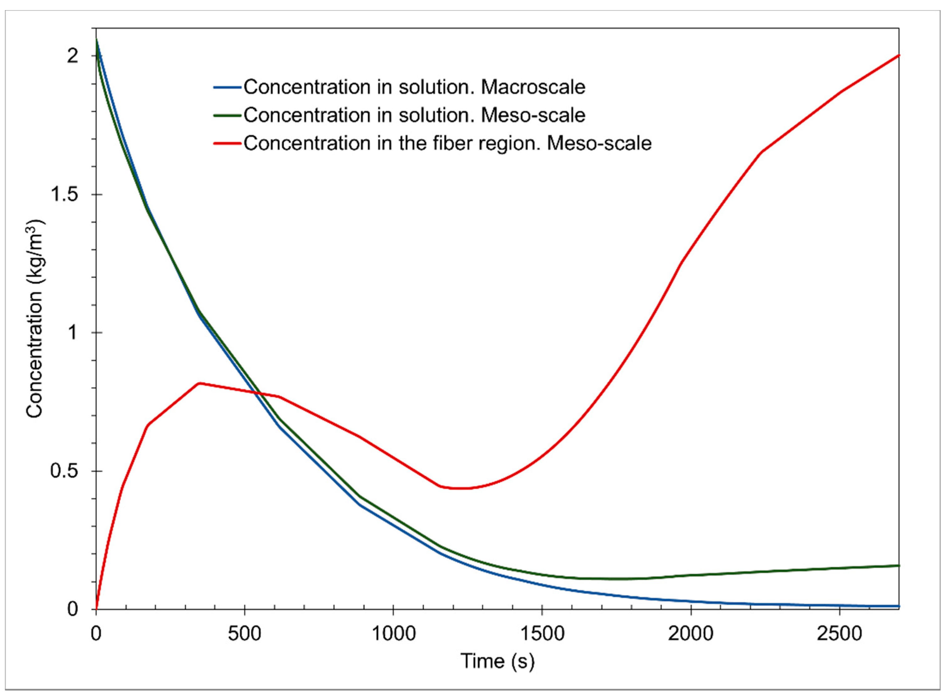
The graph of Figure 4 shows the concentrations of the dye solution on the macroscale and mesoscale, as well as the concentration in the cotton fiber on the mesoscale of the simulation of the dyeing process with the dye “C.I. Reactive Orange 107” in a 2700 s interval, with initial concentration conditions of 0.408 kg/m³ in the solution and 0 kg/m³ in the cotton fiber.

The concentration in the macroscale solution has a decreasing behavior, indicating that it is transferred towards the cotton fiber and that the dye reacts with the fiber surface in the different stages of the process. It occurs rapidly in the first 1200 s, the exhaustion stage, where only the dyeing by diffusive and convective effects occurs. In stages 2 and 3, fixing steps, the concentration slowly decreases because the dyeing occurs mainly by the reaction of the dye on the surface of the fiber. It tends to equilibrium, maintaining a concentration of 0.00735 kg/m³ on the macroscale.

In Figure 4, the concentration in the mesoscale solution is slightly higher than the macroscale concentration. This may be due to boundary conditions 2 of the mesoscale mass conservation Equation (5). This shows that adsorption due to diffusion occurs from the solution to the fiber and vice versa. This helps us to understand that in the representative volume element, there is a constant exchange of the dye in both directions due to a pressure gradient. This is described in the conservation of mass equation in the convective term Equation (3). Like the behavior of the mesoscale solution, the concentration decreases rapidly up to 1200 s and then tends to physical equilibrium with a value of 0.0321 kg/m³.

The concentration in the cotton fiber on the mesoscale has a behavior that accurately indicates the stages of the cotton dyeing process. The first stage, which is an interval from 0 to 1200 s, shows the concentration of the dye in the cotton fiber influenced only by diffusive phenomena, where only the adsorption of the dye in the cotton fibers occurs, as explained by Śmigiel-Kamińska et al. [15]. Additionally, due to the addition of salt (NaCl), forming an electrolytic solution, solvation of the dye is caused, preventing an unwanted reaction between the dye and water (hydrolysis). Therefore, we reached a maximum value at the peak of the concentration function in the cotton fiber of 0.1627 kg/m³ at 350 s in this first stage.

In the second stage, it occurs from 1200 to 2100 s, starting with a value of 0.0902 kg/m³ and ending with a value of 0.24167 kg/m³. An increase in the concentration in the fiber is appreciated due to the reaction of the dye with the surface of the cotton fiber, fixing stage, this product of the increase in pH, consequent to the addition of calcium carbonate (CaCO₃). Since the increase in the concentration of CO₃²⁻ ions, and when they dissociate, forming OH⁻ ions and the bicarbonate ion HCO₃⁻, they break the dissociation balance of the hydroxyl groups of cotton by reacting with an H⁺ ion, which forms molecules of water and carbonic acid H₂CO₃. Through this mechanism, a higher concentration of the nucleophile of the cotton fiber remains, which makes it more available for attack by the dye. This is due to the depletion stage that brings it closer to the surface of the cotton fiber, as Lewis [19] explains, on a general reactive dye reaction mechanism.

The third stage begins at 2100 s with a value of 0.24167 kg/m³ in the fiber and ends at 2700 s into the process, reaching a concentration equilibrium of 0.365 kg/m³. A slight increase in the concentration in the fiber is appreciated due to the reaction of the dye with the surface of the cotton fiber and the hydrolysis reaction, this product of the increase in pH, due to the addition of sodium hydroxide (NaOH). By further increasing the concentration of OH⁻ ions, there will be better conditions for the reactions between the dye and the cotton fiber and the hydrolysis reaction. In the simulation, these steps obtained are due to the computational code used since the respective reaction constants are added, which affect the reaction kinetics of the dyeing process for the reactive dye used.

4.3. Comparison of Experimental Data and Simulated Data

In the first comparison, with the same simulation parameters shown above, we changed only the initial conditions to match the conditions of the compared models. The concentration of the dye solution at minute 20 is 0.235 kg/m³ and the concentration in the cotton fiber is 0.0902 kg/m³. In order to emphasize the reactive effects of the dye used, there is only experimental data after 20 min (Figure 5).

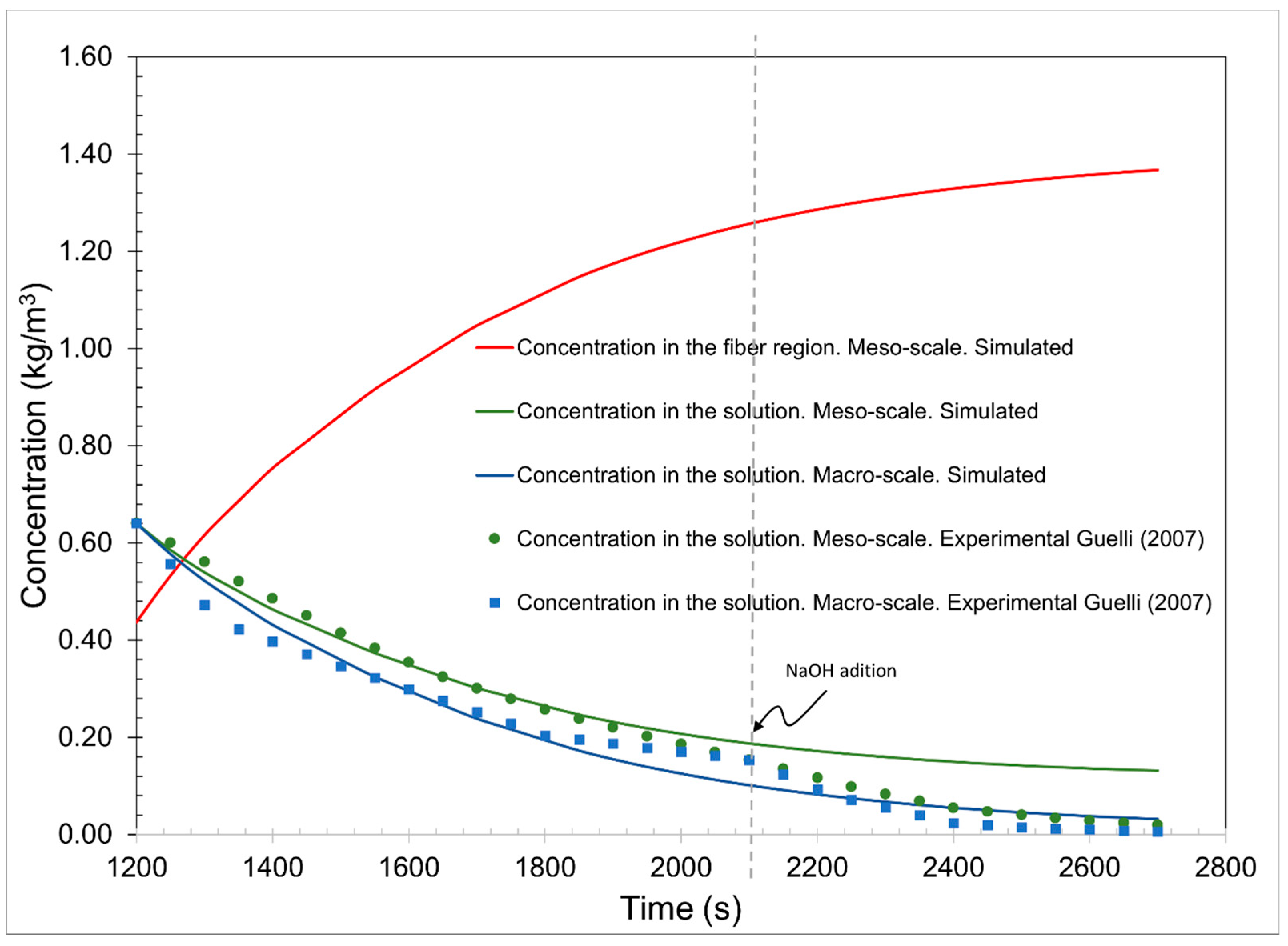
The comparison of results is shown in Figure 5. The concentration in the solution with experimental data shows the change in the decrease at 2100 s due to the increase in pH in the last stage and everything in these stages.

For the second comparison, another initial concentration presented in the base article was used. With the same simulation parameters, changing only the initial conditions to equal the conditions of the models compared, the concentration of the dye solution in minute 20 is 0.6409 kg/m³ and the concentration in cotton fiber is 0.0902 kg/m³. This is because we only had experimental data after 20 min to emphasize the reactive effects of the dye used (Figure 6).

In the concentration of both graphs, the solutions in the macroscale and the mesoscale have similar behaviors to the experimental data. However, the change at the beginning of the third stage is not appreciated. It is appreciated that both comparisons have similar behavior to the experimental data and those simulated in the article by Guelli et al. [11].

4.4. Simulation of the Curcumin Dyeing Process

In the implementation of the simulations, it was deactivating the reactive term and activating the adsorptive term of the cotton fiber mass conservation equation. Therefore, the variable ψ was assigned the value of 0 and the variable Ω was assigned the value of 1. This causes the second and fourth term from the right in Equation (3) and the third and fourth term from the right in Equation (7) to be multiplied by 1 or 0. The behavior of the concentration of the natural dye in the different phases of the process was obtained.

The cotton dyeing process with the natural dye, curcumin, was simulated with an initial concentration of 1 kg/m³ at a temperature of 70 °C. It was used as an adsorption isotherm that, based on the studies of Haque et al. [21], has higher performance in dyeing. The simulation was carried out with the parameter values in Table 2, in a time interval of 1800 s (30 min), considered for the exhaustion of the dye solution and the subsequent comparison with the experimental data. It obtained the following results.

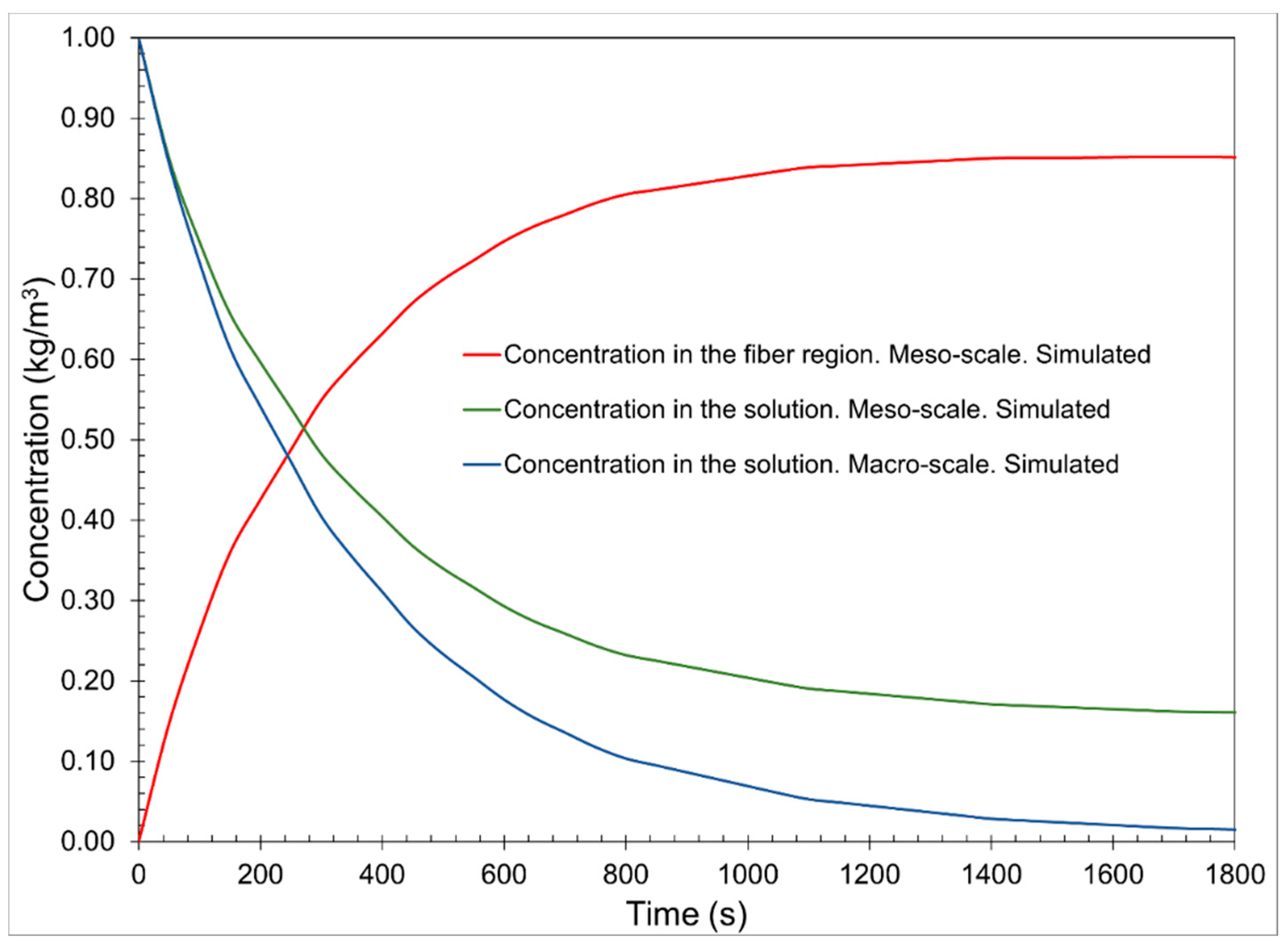
Figure 7 shows the concentration profile of the dye solution at the macroscale and the mesoscale and the concentration in the cotton fiber at the mesoscale on simulation of the dyeing process with curcumin, in an 1800 s interval with initial conditions of concentration 1 kg/m³ in the solution and 0 kg/m³ in the cotton fiber.

The concentration profile in the solution of the macroscale has a decreasing behavior, indicating the adsorption that is carried out towards the cotton fiber. The concentration profile in the solution of the mesoscale has a very similar behavior. However, there is a greater concentration when equilibrium is reached. This can be explained because, in the dye exhaustion stage, the dyeing is carried out with a lower concentration of the solution, as indicated by the macroscale. However, in reality, it is not practical dyeing since due to the affinity characteristics of the curcumin and cotton dye, there is a washout of the dye that occurs in another stage unrelated to the process. The concentration that indicates the concentration profile of the mesoscale solution is the dye that remains impregnated but not totally adsorbed in the porous medium of the fiber, and that is subsequently released in the washing stage.

The fiber concentration profile at the mesoscale increases in the first 1200 s. The three concentration profiles reached equilibrium after 1800 s.

The simulation results are obtained through approximate data based on the validation parameters of the process with the reactive dye and experimental parameters with a slight difference in the conditions of the dyeing process. With this clarification, a comparison was made between the results obtained and the experimental results of Haque et al. (2018) of the dyeing of curcumin in cotton fiber.

The data on the curcumin concentration profile in the cotton fiber were taken and converted to units of grams of curcumin per gram of cotton. For this, the volume of the fluid (7 L) plus the volume of the cone was used (0.455 L) and the mass of the cotton cone (700 g). All these values were obtained by employing the solution and fiber ratio. It was obtained from the following comparative graph.

Figure 8 shows the comparison of curcumin profiles in cotton obtained experimentally and simulated. This comparison is supported because the model developed starts from the micro and mesoscale, similar to any cotton dyeing. Similar behavior is observed, but with a slight difference in the magnitudes of curcumin concentration in cotton. These results of the developed model and its subsequent simulation with these conditions indicate that the prediction of the behavior of the concentration in cotton fiber is correct and that adjusting the experimental parameters, as a result, will result in a higher accuracy being obtained in the simulation.

5. Conclusions

In this document, a continuous mathematical model was used to simulate two different cone cotton dyeing processes. The model considers three scales, micro, meso, and macro, obtaining four equations.

The parameters of the adsorption isotherms and independent variables of the cotton dyeing process with Curcuma longa were obtained with bibliographic data. The system of equations that integrates the developed model was selected, adding a continuity equation in the fluid, considering the law of Darcy for dyeing simulation, which gives simulation variants to the model based on the characteristics of the fiber to be used. Due to the physics of the process, changes were also made to the mathematical reference model, mainly to the reactive term of the cotton fiber mass conservation equation in the mesoscale for optimal behavior, as indicated by the reaction mechanisms to use a reactive dye.

The simulations were validated with bibliographic data for the dyeing processes of reactive dye “C. I. Reactive orange 107”, with an initial concentration of 0.408 and 2.06 kg/m³. An RMSE of 0.00221 and 0.0289 kg/m³, respectively, was obtained, indicating a great absolute fit and precision of the experimental data and the data obtained from the simulation. Regarding the comparison of data from the dyeing process with curcumin, there is a slight data deviation since there are no experimental data of the conditions of the dyeing process. However, it has similar behavior, and adjusting these parameters will obtain a higher model accuracy for curcumin staining.

These results validate the model used in this work, breaking down the critical phenomena and stages of the dyeing process, such as adsorption, diffusion, and reaction, which depend on the dye used. For reactive dyes, based on the profile of the reactive term obtained, it is essential to control the reaction constants of the process, forcing the lowest possible hydrolysis kinetics to be had, favoring a more significant reaction of the dye and the surface of the cotton fiber.